Research Collection
Bachelor Thesis
Restoration and Reconstruction of 3D cryo-EM Images
Author(s):
Agarwal, Ishaant Publication Date:
2021-04
Permanent Link:
https://doi.org/10.3929/ethz-b-000480083
Rights / License:
In Copyright - Non-Commercial Use Permitted
This page was generated automatically upon download from the ETH Zurich Research Collection. For more information please consult the Terms of use.
ETH Library
Restoration and reconstruction of 3D cryo-EM Images
Undergraduate Thesis
Submitted in partial fulfillment of the requirements of BITS F421T Thesis
By
Ishaant Agarwal ID No. 2016B5A30103G
Under the supervision of:
Dr. Simon Nørrelykke
&
Dr. Ashish Chittora
BIRLA INSTITUTE OF TECHNOLOGY AND SCIENCE PILANI, KK BIRLA GOA CAMPUS
April 2021
Declaration of Authorship
I, Ishaant Agarwal , declare that this Undergraduate Thesis titled, ‘Restoration and reconstruc- tion of 3D cryo-EM Images ’ and the work presented in it are my own. I confirm that:
This work was done wholly or mainly while in candidature for a research degree at this University.
Where any part of this thesis has previously been submitted for a degree or any other qualification at this University or any other institution, this has been clearly stated.
Where I have consulted the published work of others, this is always clearly attributed.
Where I have quoted from the work of others, the source is always given. With the exception of such quotations, this thesis is entirely my own work.
I have acknowledged all main sources of help.
Where the thesis is based on work done by myself jointly with others, I have made clear exactly what was done by others and what I have contributed myself.
Signed:
Date:
i
Certificate
This is to certify that the thesis entitled, “Restoration and reconstruction of 3D cryo-EM Images
” and submitted by Ishaant Agarwal ID No. 2016B5A30103G in partial fulfillment of the requirements of BITS F421T Thesis embodies the work done by him under my supervision.
Supervisor
Dr. Simon Nørrelykke Group leader,
ETH Zurich Date:
Co-Supervisor
Dr. Ashish Chittora Asst. Professor,
BITS Pilani, Goa Campus Date:
ii
“Careful. We don’t want to learn from this.”
Bill Watterson, “Calvin and Hobbes”
BIRLA INSTITUTE OF TECHNOLOGY AND SCIENCE PILANI, KK BIRLA GOA CAMPUS
Abstract
Bachelor of Engineering (Hons.)
Restoration and reconstruction of 3D cryo-EM Images
by Ishaant Agarwal
Cryogenic electron microscopy (cryo-EM) has emerged as the preferred method for imaging
macromolecular structures. Like most other high-powered imaging techniques it suffers from
a trade-off between acquisition time and quality. Traditional denoising methods for cryo-EM
include averaging and Fourier cropping. They are not only resource-intensive, but also lose
out high frequency details. Other denoising methods rely on constructing a model of the noisy
process and rely on simplified assumptions. In this study, we train a neural network to model
the noisy process and output denoised 3D cryo-EM density maps while minimizing the loss of
high frequency components; even in the absence of ‘clean’ target maps for training.
Acknowledgements
Throughout the writing of this thesis I have received unimaginable support and assistance.
Firstly I would like to thank my supervisors Drs. Simon F. Nørrelykke and Andrzej Rzepiela.
They have been excellent mentors and have offered me guidance all the way, motivating me to learn new things and better myself each day. Even in a world upheaved by the pandemic, they found a way for me to join them in Zurich and even funds to support my stay.
I am also immensely grateful to all the other members of IDA: Dr. Szymon Stoma for his insightful feedback and carefully making sure I did not lose focus (as I am wont to!), Dr. Nelly Hajizadeh for helping me get set up and ideate during the early and more stressful stages of my stay and to Joanna Kaczmar for lending her exceptional programming expertise and helping me with innumerous tasks.
I would also like to show my gratitude to my on-campus guide Prof. Ashish Chittora for agreeing to supervise me on extremely short notice, whilst also grappling with a much more hectic work schedule.
Getting through my thesis required more than academic support, and I have many, many people to thank for listening to and, at times, having to tolerate me over the past few months. Saumya, for being my rock and playing up very small bit of progress. You kept me motivated through all ups and downs; Rishab, who was always willing to lend an ear, a hand and half a foot whenever I thought myself stuck with no recourse; and my family for supporting me and always being there- a crutch to lean on.
Finally, I want to acknowledge the help provided to me by Fran¸ coise at ScopeM, the Student Exchange Office and all other members of ETH and ScopeM who made my research stay possible seamlessly.
v
Contents
Declaration of Authorship i
Certificate ii
Abstract iv
Acknowledgements v
Contents vi
List of Figures viii
1 Introduction 1
2 Theory 3
2.1 Noise2Noise . . . . 3
2.2 Loss functions . . . . 4
2.2.1 Mean Squared Error (MSE) . . . . 4
2.2.2 Absolute Error/L1 Loss . . . . 4
2.2.3 Fourier Shell Correlation (FSC) . . . . 4
3 Results 6 3.1 Testing . . . . 6
3.1.1 2D Model . . . . 6
3.1.2 Simple 3D Model . . . . 7
3.2 Main Model . . . . 11
3.2.1 Initial Training . . . . 11
3.2.1.1 Scenario 1 . . . . 11
3.2.1.2 Scenario 2 (with lower learning rate) . . . . 13
3.2.2 Changes . . . . 14
3.2.3 Final Training . . . . 16
3.2.3.1 Scenario 3- Minimum Zero Shift . . . . 16
3.2.3.2 Scenario 4- Mean Zero Shift . . . . 17
3.2.3.3 Scenario 5- Standardization . . . . 17
vi
Contents vii 3.3 Stitching Script . . . . 19
4 Discussion 22
A Supplementary Information 24
B Code 26
Bibliography 32
List of Figures
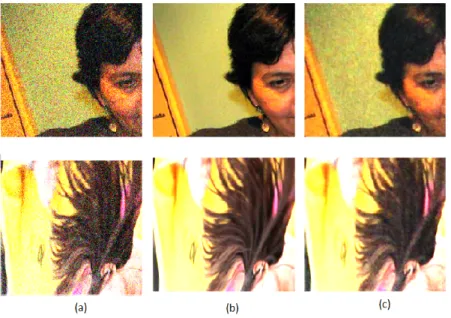
3.1 Samples showing the performance of the 2D network on two images. a)noisy measurements of the clean images shown in b). c) is the output of the denoising network on the same images. We enhanced the contrast of these images using Fiji[27] for better visualization. . . . . 7 3.2 2-D slices from an example training dataset patch a) Slice from 3D Map before
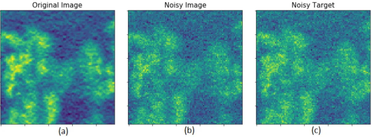
adding noise. b) Slice of input patch obtained by adding Gaussian noise (mean=0, σ 2 =0.01) to (a) c) Slice of target patch obtained by adding similar Gaussian noise to (a) . . . . 8 3.3 Samples showing the performance of the 3D network on two image patches. a)
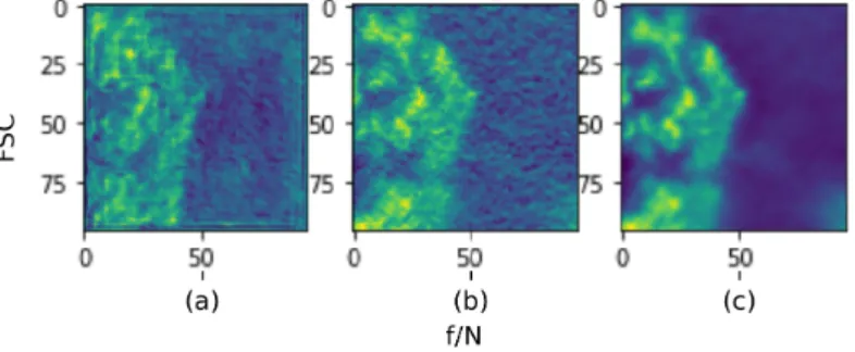
Slice from 3D Map before adding noise. b) Slice from input patch obtained by adding gaussian noise (mean=0, σ 2 =0.01) to a c) Slice from the output of the denoising network on the same patch . . . . 9 3.4 FSC Curves for both c) and e) datasets. f /N denotes frequency normalized by
the Nyquist frequency for the images. The Clean-Noisy line represents the FSC between the input to the network and ground truth while the Clean-Denoised line represents the FSC between the ground truth and the network’s output. For comparison, the Original-Averaged line shows the FSC score between the mean of all training images and ground truth. Since we use a zero-mean gaussian noise, the average image is expected to be the same as the original/clean image, as evidenced by the unitary FSC score. We observe that the network obtains an equally impressive FSC improvement across all frequencies in both N2N and N2GT scenarios. . . . . 9 3.5 FSC curves for both d) and f) datasets. f /N denotes frequency normalized by the
Nyquist frequency for the images. We observe again that the FSC improvement for both N2N and N2GT networks are comparable. . . . . 10 3.6 2-D slices showing the results of scenario 1 a) Slices from ”clean 3D test patch”.
b) Corresponding input patch slices c) Slices from the output of the denoising network on the same patch . . . . 12 3.7 FSC Scores for Scenario 1 for two different patches from the test half-map. Note
that the FSC for the denoised image is lower than that of the noisy input half-map lower for higher frequencies. A possible explanation for this is that the the original patch is constructed by processing a combination of both input and target half-maps, and hence could contain noise from the latter. On visual inspection the clean patch does seem like it contains noisy artifacts. (Ref figure 3.6) . . . . 12 3.8 Slices of a) Output of network before training b) Input patch and c) Output of
network after 1k training iterations . . . . 12 3.9 FSC Scores for denoising the test patch, seen as a function of number of training
iterations for (A) Scenario 1 and (B) 2. We observe that the improvement in FSC was much steadier, albeit slower, with the lower learning rate in (B). . . . . 13
viii
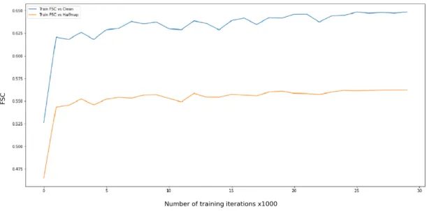
List of Figures ix 3.10 MSE Training Loss comparison between Scenarios 1 and 2 over 60k iterations . . 14 3.11 Average FSC scores for scenario 3 on training miniset over training period. X
ticks are present in units of 1k iterations. It can be seen that the FSC scores with both the clean ad paired noisy half-map have very similar trends. This indicates that the higher score with the clean patch is both due to the absence of noise and because the clean map is made through processing a combination of both input and target half-maps. Also note that the FSC score saturates after the 27k iteration mark. . . . . 16 3.12 FSC Score for Scenario 3 on the same test patch used in initial training. (Ref figure
3.7) Our output does not have any contextual information about the Noisy2 patch.
The improvement can be seen as both the improvement from the Clean-Noisy1 (Green) to the Clean-Denoised1 (Blue) line and as the improvement between the
Noisy2-Noisy1 (Orange) to the Noisy2-Denoised1 (Red) line. . . . . 17 3.13 Average FSC scores for scenario 5 on training miniset over training period. X
ticks are present in units of 1k iterations. We find that the network learns much faster and converges at a lower loss when inputs are standardized. . . . . 18 3.14 Slice from a half-map that was denoised patch-by-patch. (B) and (C) show the
final recombined image with and without window-based stitching. The network from scenario 5 was used as the denoiser. The denoising script is successfully able to stitch network output patches together to form a whole 3D image while eliminating artifacts generated otherwise. This image can directly be used to visualize the 3D structure in an external tool like UCSF Chimera[23] . . . . 21 A.1 3D UNet Network Architecture of the main model. The numbers alongside denote
the shapes of weights of convolutional layers as well the the network’s input and
output sizes. Deconvolution layers are identical to the 3D convolutions layers in
construction. All leaky ReLUs are initialized with α = 0.1. . . . . 25
To Saumya, books, video games and Switzerland
x
Chapter 1
Introduction
Image denoising aims to recover a high quality image from its noisy/degraded observation. In the last several years, deep neural networks (DNNs) [] have achieved great success on a wide range of computer vision tasks (e.g., [10, 12, 26, 28]). Unsurprisingly, DNNs have been employed for denoising as well [13, 18, 32, 7]. Conventional Artificial Intelligence (AI)-based solutions utilize pairs of noisy and clean images (as input and target) for training [31, 17, 33]. Caveat: No truly ”clean” image actually exists for real world data. To work around this problem, datasets consist of images that are 1) generated synthetically [6, 34] or 2) denoised using traditional image processing techniques like spatial filtering, long exposure averaging, Fourier cropping etc [13, 25].
Recently, there has been incredible work done in developing denoising neural networks that do not require ground truth images [7, 18, 13]. Noise2Noise (N2N) [18] is a deep learning algorithm that leverages knowledge about noise statistics to learn to generate denoised ”clean” images by only looking at noisy images. This has significant applications for any imaging technique where generating clean data requires long imaging sessions and manual tuning of acquisition parameters.
We believe cryogenic Electron Microscopy (cryo-EM) imaging has the potential to benefit significantly through incorporating an N2N-based denoising pipeline. cryo-EM can be used to determine the three-dimensional structure of biomacromolecules in frozen states at close to atomic resolution, and has the potential to reveal conformations of dynamic molecular complexes[21].
We can use neural networks to greatly improve the quality (resolution and signal-to-noise ratio) of acquired images, reducing the acquisition time and facilitating the capture of high-resolution images on lower-resolution microscopes.
Even though work has been done recently, in deploying N2N based solutions for cryo-EM [5, 22], they have used locally generated data (using their own microscopes) for training, thereby limiting their use and scope. Moreover, these approaches generally deal with 2-D images, thereby losing
1
Chapter 1. Introduction 2 contextual information. Furthermore, current methods optimize the Mean Squared Error loss function which undervalues higher frequency information during the denoising process. Therefore there is currently a lack of work that deals with 1) the preservation of high frequency data while denoising 3D cryo-EM images and 2) doing so using 3D patches, instead of 2D slices. We seek to remedy this gap in literature.
The contributions in this thesis are threefold:
1. cryo-EM images are particularly suited for N2N denoising as the 3D image frames can be split into even and odd “half-maps” having independent noise and thus can be used as input-target pairs (ref. Theory 2). The Electron Microscopy Data Bank [15] contains thousands of half-maps submitted by hundreds of groups- a promising and (as of yet) underutilized training dataset. This lets us build a data-agnostic denoising network, that generalizes well to different kinds of imaging protocols, equipment and resolutions. To our knowledge, no work has yet utilized the EMDB images to train a cryo-EM denoising network.
2. We exploit efficiencies in TensorFlow [1] that let us load large 3-D patches onto GPU for network training and processing by preprocessing datasets into tfrecords files. This lets TensorFlow internally use Protocol Buffers to serialize/deserialize the data and store them in bytes, as it takes less space to hold an ample amount of data and to transfer them as well [4]. Bigger patches give more context for each voxel, and lead to lesser number of patches overall, limiting the generation edge artifacts. We augment this by developing a
“stitching script”, based on recent literature [24], to recombine the patches into a single map while eliminating most edge artifacts.
3. We utilize a new measure of loss, based on the Fourier Shell Correlation score[9], that has been shown to improve network performance, especially while tackling the loss of information at higher frequencies.[8]
We are, therefore, able to design a network that can successfully denoise whole cryo-EM
images, from different settings, without generating any obvious artifacts.
Chapter 2
Theory
2.1 Noise2Noise
Noise2Noise[18] uses a UNet[26] neural network architecture to denoise different kinds of images without using any ground truth. Consider that a neural network is fed in some input with the goal of generating a target output. For a conventional denoising network, the input would be raw, noisy images and targets would be clean/denoised images.
In Noise2Noise, Lehtinen et al. feed pairs of noisy images as both input and target. They demonstrate that for a dataset consisting of such noisy pairs, the network will converge to the same parameter values as a conventional Noise2Clean approach, given that the noise between pairs is uncorrelated and has zero mean or median. In cryo-EM imaging most noise is shot noise [3]. Shot noise, also known as Poisson noise, is not correlated between observations. Hence N2N can be applied to these images.
Mathematically, if an image is represented by
I = S + N (2.1)
where S is the signal present in the image and N is the noise. Then for images
I 1 = S + N 1 and I 2 = S + N 2 (2.2)
shot noise in cryo-EM half-maps fulfills the relations
P (N 2 |S, N 1 ) = P (N 2 |S) (2.3)
E(N 1 ) = E(N 2 ) = 0 (2.4)
3
Chapter 2. Theory 4 where P(A|B) denotes the conditional probability of A, given B. The first relation (Eq 2.3) implies that noise measurements between half-maps are pixel-wise uncorrelated. The second relation (Eq 2.4) implies that the average expectation value of the noise is 0 - these are the main prerequisites for N2N denoising to be applicable.
2.2 Loss functions
2.2.1 Mean Squared Error (MSE)
The noise of an image is generally qualified by the MSE, also known as L2 loss. For images, it can be calculated as
M SE(I 0 , I) = 1 N ∗
N
X
i=1
(I 0i − I i ) 2 (2.5)
where the sum is over all pixels i of an image. I 0 and I represent pixel intensities of clean and noisy images respectively. MSE is based on pixel-wise error and is a good measure for datasets having zero mean noise. MSE has a lower bound of 0 and upper bound given as the sum of absolute maximum pixel intensities of each image, i.e |max(I 0 )| + |max(I)|
2.2.2 Absolute Error/L1 Loss
L1 loss, as may be discerned, is similar to MSE (L2) loss. It also based on pixel wise difference between images. However, L1 is calculated as the mean of the modulus of their difference.
L1(I 0 , I ) = 1 N ∗
N
X
i=1
|I 0 i − I i | (2.6)
with I, I 0 and N representing the same objects as in MSE (equation 2.5). It is used as a loss function when N2N deals with noise that is zero-median[18] instead of zero-mean. However, we have not used L1 loss for reporting any results in this thesis so far. We mention it to show that different loss functions can be better suited to deal with different noise types, at least in N2N.
2.2.3 Fourier Shell Correlation (FSC)
Fourier Shell Correlation (FSC)[9] and its 2-D counterpart Fourier Ring Correlation (FRC)
measures the normalized cross-correlation between two volumes(/images) over corresponding
shells(/rings) in the Fourier domain. It measures the similarity of signals between two images as
a function of frequency. The FSC value between two image volumes is given by [8]
Chapter 2. Theory 5
F SC (S) =
P
r∈S F 1 (r) · F 2 ∗ (r) p ( P
r∈S |F 1 (r)| 2 ) · ( P
r∈S |F 2 (r)| 2 ) (2.7) where F 1 and F 2 ∗ represent the Fourier transform and conjugate Fourier transform of the two images respectively, S is the shell being considered. The summation is performed over all frequency spheres contained in the shell S. To calculate a scalar score, we integrate the FSC score over all frequency shells upto the Nyquist frequency.
F SC scalar = Z f
0
F SC(S) dS (2.8)
It can range from 0, for completely uncorrelated images, to 1 for perfectly correlated images.
Negative values (upto -1), imply an inverse correlation. Since this is a similarity score, we use the expression
Loss F SC = 1 − F SC scalar (2.9)
as our loss function. Therefore 2 represents the maximum loss and 0 represents no loss. Typically the loss is a value less than 1.
Hajizadeh et al.[8] show that FRC/FSC act as better loss functions when training networks, optimizing faster than MSE. We also observe that since MSE places equal weight on each pixel, and since low-frequency signal information is encoded over more pixels than high-frequency signal, the latter is often lost (due to uneven weighing) when optimizing MSE loss.
Unlike MSE note that FSC is scale invariant, since it only measures correlations. It does not restrict the network output to have the same scale as the input or target. Therefore, normalizing the network output is necessary to perform any analysis/calculations dependent on pixel intensities (such as calculating MSE). This is done automatically in our stitching script.
(refer section 3.3)
Chapter 3
Results
The results are divided into three sections - 1) Testing, 2) the Main Model and the 3) Stitching Script. The main model refers to the 3D network trained on our final dataset after conclusion of the test phase.
In (3.1) Testing, we implement simple 2D and 3D N2N models. Both of these are sanity checks to ensure that we are actually able to denoise images. The second is especially important since we do not have any guarantee of N2N denoising working well with large 3D patches.
(3.2) Main Model describes the dataset construction and training methods we use to develop a network that can denoise 3D cryo-EM images acquired using several different imaging protocols.
We explain the insights discovered during training and the changes these led to.
Finally the (3.3) Stitching Script section describes in detail our need for, and implementation of, a method that combines patches to form single coherent images while eliminating edge artifacts.
3.1 Testing
The initial stage of the project involved testing the existing codebase to whittle out bugs and ensure that the neural network could be trained correctly. We started by training the default 2D model from the Nvidia N2N repository[18] and then moved on to a simple 3D network. All networks were trained using the Adam Stochastic Optimizer[11].
3.1.1 2D Model
The network was trained on images from the Google Open Images[14] dataset. The images were of different sizes with 3 8-bit channels (RGB). We converted the pixel intensities to float values
6
Chapter 3. Results 7 in the range [0,1] and generated two independent noisy observations of 256 randomly selected images from the dataset by adding zero-mean Gaussian Noise with variance σ 2 = 0.01. These images were cropped to a size 256x256 and used to train the network for 1000 iterations.
Figure 3.1: Sam- ples showing the perfor- mance of the 2D net- work on two images.
a)noisy measurements of the clean images shown in b). c) is the output of the denoising network on the same im- ages. We enhanced the contrast of these images using Fiji[27] for better
visualization.
The network was able to reduce the Mean Squared Error by 83%, from 0.3 to 0.05, without ever being fed the clean targets.
3.1.2 Simple 3D Model
We tested the 3D network by generating a synthetic dataset and verifying if the network was able to denoise a single protein half-map. We also looked at different hyper-parameters and their effects on training.
Dataset Preparation
We manually selected a patch of 64x64x64 voxels from a random protein half map, belonging to the EMDB database [15]. We wanted to investigate how the training dataset size would affect the performance of the network- how much data constitutes the bare minimum and how much would be excessive. Therefore, we added Gaussian noise to the image and generated three datasets containing a) 1,000, b) 10,000 and c) 30,000 pairs of independent noisy observations.
The voxel values were normalized to a range [-0.5,0.5]. Then, we prepared two more datasets d) and e) containing 10,000 and 30,000 image pairs respectively, but with the original image (Ground truth) as the target, i.e., N2GT. The noise statistics are mean 0, σ 2 = 0.01 for {a,b,d}
and σ 2 = 0.07 for {c,e}.
In the subsequent parts of this section we will refer to each training configuration as indexed by
the dataset, {a-e}
Chapter 3. Results 8
Figure 3.2: 2-D slices from an example training dataset patch
a) Slice from 3D Map before adding noise. b) Slice of input patch obtained by adding Gaussian noise (mean=0, σ
2=0.01) to (a) c) Slice of target patch obtained by adding similar Gaussian
noise to (a)
Training
Since these images are 3-dimensional, we modified the earlier network, 2D CNN network, to have 3D convolution kernels. We give the training and Test Loss for all N2N datasets below.
The training parameters are given in the Appendix. Datasets a-c were trained with both noisy inputs and noisy targets (“N2N”), while d,e had noisy inputs with clean targets (N2GT). For testing, we generated a new noisy measurement from the same distribution each time, and used it as input for the network.
Dataset Training Loss (MSE) Test Loss (MSE) Test FSC Score Dataset Type and Size
a 0.0118 0.027 - N2N 1k
b 0.0044 0.025 0.855 N2N 10k
c 0.0179 0.014 0.86 N2N 30k
d 0.00098 0.003 0.852 N2GT 10k
e 0.00117 0.004 0.872 N2GT 30k
Table 3.1: Loss and FSC values for the different datasets
Analysis
We confirmed our initial hypotheses that the network performed better with more
data (validation loss decreases from datasets b-d). To the extent of our experiments,
more data was always helpful. Furthermore, although the Ground Truth formulation did
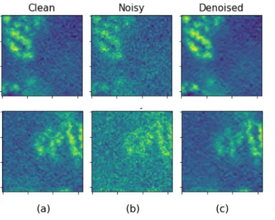
Chapter 3. Results 9 Figure 3.3: Sam- ples showing the per- formance of the 3D network on two image patches. a) Slice from 3D Map before adding noise. b) Slice from in- put patch obtained by adding gaussian noise (mean=0, σ
2=0.01) to a c) Slice from the output of the denoising network
on the same patch
have lower MSE, we compared the FSC scores between them as well, on a test patch. c) N2N with 10k noisy pairs scored a 0.855 FSC, which is very close to the FSC score of its corresponding N2GT network e) 0.86 (refer figure 3.4). Note that these values are a 40% improvement over the original FSC score of 0.62 between the ground truth and input image.
(a) FSC Curve for c) N2N with 10k pairs (b) FSC Curve for e) N2GT with 10k pairs
Figure 3.4: FSC Curves for both c) and e) datasets. f /N denotes frequency normalized by the Nyquist frequency for the images. The Clean-Noisy line represents the FSC between the input to the network and ground truth while the Clean-Denoised line represents the FSC between the ground truth and the network’s output. For comparison, the Original-Averaged line shows the FSC score between the mean of all training images and ground truth. Since we use a zero-mean gaussian noise, the average image is expected to be the same as the original/clean image, as evidenced by the unitary FSC score. We observe that the network obtains an equally impressive
FSC improvement across all frequencies in both N2N and N2GT scenarios.
We also observed even better results for the 30k image datasets (refer figure 3.5). with d) and f) garnering FSC scores of 0.852 and 0.872, even though they dealt with significantly more noise.
This was an improvement of 70% over the original FSC score of 0.513 between the Ground truth
Chapter 3. Results 10 and noisy input. Therefore, we can see that our network can denoise even severely degraded images.
(a) FSC Curve for d) N2N with 30k pairs (b) FSC curve for f) N2GT with 30k pairs
Figure 3.5: FSC curves for both d) and f) datasets. f /N denotes frequency normalized by the Nyquist frequency for the images. We observe again that the FSC improvement for both N2N
and N2GT networks are comparable.
Therefore, we make two observations:
1. Our network can denoise simple 3D datasets, even when the images are severely degraded.
2. N2N performs similar to N2GT when a quality measure different from the loss function
(FSC here) is used as the metric.
Chapter 3. Results 11
3.2 Main Model
Dataset
For the main model, we collected all records submitted to the Electron Microscopy Data Bank [15] which had at least two half-maps, as of 8 February 2020. Each half map can be thought of as an independent noisy measurement of the structure signal. Hence, we had 1297 pairs of half-maps for a variety of structures. We did not preprocess these in any way other than to break them into patches that could be fit onto the GPU and normalizing the inputs when fed to the network. More information about the normalization is detailed for each training scenario in the relevant sections. All the datasets created hereon consist of patches sized 96x96x96.
We created the training dataset D 1 comprising 57k pair of patches from these half-maps.
We updated our dataset on 10 November 2020 which got us 341 additional structure half map pairs. They were set aside to be used as a test set.
3.2.1 Initial Training Exploratory Training
We first trained the network on all patches for 10 4 iterations. However, the loss function curve was still decreasing at the end of training. This indicated that the network had not converged and training was unfinished. Therefore we revised the training setup by increasing the batch size and number of training iterations, as detailed below. Furthermore, we selected one test patch unseen by the network and compared our output with a half-map cleaned by the authors using traditional image processing methods, including superposition of multiple half-maps.[19]. The patch extracted from this half-map is hereon called the ‘clean test patch.’ The initial training consisted of two scenarios.
3.2.1.1 Scenario 1
We trained the N2N network for 6E4 iterations with a batch size of 36 and 3.0E-4 learning rate.
The input and target patches were all normalized individually so that their voxel intensities
ranged between [-0.5,0.5] with 0 mean. They were also shuffled randomly before being loaded
for training. Although the output pictures for a test patch looked visually appealing (see figure
3.6), the loss function was fluctuating considerably (even though its the moving average was still
decreasing.) Therefore, it was reasonable to assume it would benefit from a lower learning rate
and possibly converge further. The training MSE was approximately 0.002 at the final iteration.
Chapter 3. Results 12 Figure 3.6: 2-D slices
showing the results of scenario 1 a) Slices from
”clean 3D test patch”.
b) Corresponding input patch slices c) Slices from the output of the denoising network on
the same patch
(a) FSC Curve for a test patch for scenario 1 (b) FSC Curve for another test patch for scenario 1
Figure 3.7: FSC Scores for Scenario 1 for two different patches from the test half-map. Note that the FSC for the denoised image is lower than that of the noisy input half-map lower for higher frequencies. A possible explanation for this is that the the original patch is constructed by processing a combination of both input and target half-maps, and hence could contain noise from the latter. On visual inspection the clean patch does seem like it contains noisy artifacts.
(Ref figure 3.6)
It was also interesting to note that even after just 1000 iterations, the network displayed significant improvement in visual quality, although quantitative quality did improve with more training.
Figure 3.8: Slices of a) Output of network before training b) Input patch and c) Output of
network after 1k training iterations
Chapter 3. Results 13
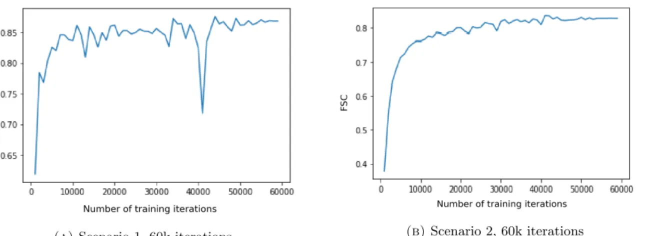
(a) Scenario 1, 60k iterations (b) Scenario 2, 60k iterations
Figure 3.9: FSC Scores for denoising the test patch, seen as a function of number of training iterations for (A) Scenario 1 and (B) 2. We observe that the improvement in FSC was much
steadier, albeit slower, with the lower learning rate in (B).
FSC scores were observed to be increasing steadily (Figure 3.9 (a)) despite minimal changes in MSE. This could be attributed to the fact that frequency components are not distributed evenly among the pixels. Low frequency components of the signal get a significantly higher “pixel-share”
than high-frequency components. Hence even these seemingly insignificant changes in MSE also lead to a significant increase in FSC scores[8].
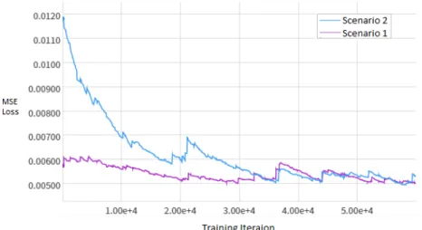
3.2.1.2 Scenario 2 (with lower learning rate)
We trained the N2N network for both 6.0E4 (as before) and 3.0E5 iterations with a lower
learning rate 3.0E-5. The batch size, normalization and shuffle were identical to that in Scenario
1. We ran training longer to check if the network would learn more or over-fit but there was no
significant improvement in training loss after 6.0E4 iterations. We scaled down the learning rate
by a factor of 10 hypothesizing that this would reduce fluctuations and let the network learn
more steadily. Even thought it succeeded in both of these, the overall loss remained unchanged
after 3.5E4 iterations. The longer 3.0E5 iteration run also had only a 4% reduction in loss
compared to the 6.0E4 run. This indicated that training longer was not yielding proportional
improvement in performance.
Chapter 3. Results 14
Figure 3.10: MSE Training Loss comparison between Scenarios 1 and 2 over 60k iterations
3.2.2 Changes
At this point we decided to make several changes to our training rules:
1. We implemented the FSC function in TensorFlow and tested it application as a loss function. Since FSC and its gradient calculation is memory-intensive we had to reduce batch size to 12 for all subsequent training.
The MSE training did well in improving the FSC for low frequencies but had limited success with higher frequency signal. Since the FSC loss function places an equal weight on all frequencies, we assumed this would increase denoising performance.
2. Instead of training networks from scratch, we would reuse networks that had already been trained with MSE loss.
MSE minimization increases FSC scores so this gives us a headstart in training. We tried pure FSC training too, but the output turned out blurry. However, continued training of an MSE-trained network with FSC loss yielded better results than both pure FSC-trained and pure MSE-trained networks. This indicates equal importance to all frequency components is not optimal for initial training. This could occur due to two reasons: i) more pixels encode low frequency data than high frequency, so the network has more data to learn from for the former. ii) Different training patches are likely to have more low frequency information in common than higher frequency (since the latter corresponds to minute details.) Therefore a loss function that prioritizes low frequency data accuracy will be more stable for the initial phase.
3. We would check the effect of different types of normalization on overall train-
ing and network performance.
Chapter 3. Results 15 In the original N2N[18] work the authors use noise of different variances while training so that the network generalizes well to denoising different amounts of noise. However, this is not a pressing requirement for our use-case since our dataset already includes data from a diverse range of sources and imaging modalities. Normalization, instead, can help prevent the network from mistakenly identifying different images, of the same type, as belonging to different contexts.
4. We created two separate test sets, since testing patches from only one map is not a good practice.
The first set T 1 consisted of 100 patches (pairs) from 50 half-map pairs that were not included in the training set. The patch coordinates for each map were picked via random Gaussian sampling. The second set T 2 comprised 20 patches that were extracted manually to ensure they had significant signal.
5. We also created a miniset of the training patches with 100 patches (pairs) picked randomly from 50 half-map pairs. This is used as a sample to evaluate performance on the training data better.
6. To reconstruct complete maps from patches, we implemented a stitching script
based on Pielawski and Walby (2020)[24]. This script automates the import of a
whole 3-D half-map (as a .mrc or .map.gz file), divide it into patches with appropriate
zero-padding, denoise them patch by patch and recombine the overlapping denoised patches
while avoiding edge artifacts.
Chapter 3. Results 16 3.2.3 Final Training
In this part we retrained the Scenario 2 network from above while optimizing the new FSC Loss function. We explored three different normalization scenarios:
3.2.3.1 Scenario 3- Minimum Zero Shift
We preprocessed each patch by subtracting its minimum. This is equivalent to shifting the voxel intensities to have a lower bound of 0. Our motivation was to check whether making the mean zero is uniquely useful, as is the case for sigmoid non-linearities[16], or if any kind of uniform offset could have the same effect. After training, we observed an average FSC increase of 19%
from the noisy pairs on the training data miniset. FSC scores here are calculated between the output of a network, and the noisy half-pair of the corresponding input. We also observed an increase in FSC scores for T 2 by 14% on average, even when FSC values were often high to begin with. This performance was comparable to - even slightly better than- the performance in Scenario 4 with a mean shift to zero.
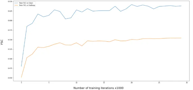
Figure 3.11: Average FSC scores for scenario 3 on training miniset over training period. X ticks are present in units of 1k iterations. It can be seen that the FSC scores with both the clean ad paired noisy half-map have very similar trends. This indicates that the higher score with the clean patch is both due to the absence of noise and because the clean map is made through processing a combination of both input and target half-maps. Also note that
the FSC score saturates after the 27k iteration mark.
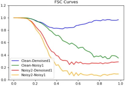
Chapter 3. Results 17 Figure 3.12: FSC Score for Scenario 3 on the same test patch used in initial train- ing. (Ref figure 3.7) Our out- put does not have any con- textual information about the Noisy2 patch. The improve- ment can be seen as both the improvement from the Clean- Noisy1 (Green) to the Clean- Denoised1 (Blue) line and as the improvement between the Noisy2-Noisy1 (Orange) to the Noisy2-Denoised1 (Red) line.
3.2.3.2 Scenario 4- Mean Zero Shift
Here, we preprocessed each input and target patch by subtracting their mean voxel intensity before being fed into the network. No scaling normalization/standardization was applied. This scenario was similar to that in the original N2N paper[18], where they trained the network to deal with noise of different variances. This gives the network an added burden of estimating the level of noise while denoising. We perform this to find out if standardization generates any significant improvement in performance for our use case.The network observed a 14.3 % increase in FSC scores for T 2 , results very similar to Scenario 3.
3.2.3.3 Scenario 5- Standardization
For the final run, we trained the network by standardizing the patches to have mean voxel intensity 0 and standard deviation 1. We observed an average FSC improvement of 15.79% on T 2
and 22% on the training miniset, which is the best performance so far. Therefore, the network performs better when the data is confined to a uniform scale. However, it is clear that making the mean zero is not uniquely useful.
Scenario Description Training Set Improvement Test Set Improvement
3 Minimum 0 Shift 19% 14.6%
4 Mean 0 Shift 20% 14.3%
5 Standardization 22% 15.8%
Table 3.2: Performance obtained through different types of normalization.
Chapter 3. Results 18
Figure 3.13: Average FSC scores for scenario 5 on training miniset over training period. X ticks are present in units of 1k iterations. We find that the network learns much faster and
converges at a lower loss when inputs are standardized.
Chapter 3. Results 19
3.3 Stitching Script
The neural network is constrained by GPU memory. It cannot load and denoise an entire map at one go; hence, we divide the maps into patches. However, while training patches the voxels near the edge(s) have lesser neighbours (and contextual information) than those at the center. This creates an information mismatch. Combining these patches independently leads to artifacts. To deal with the unequal contextual information distribution, we use overlapping patches. But this poses another challenge: how do we combine the overlapping output so that output voxels nearer the center (in each patch) are weighted higher. Pielawski and Walby (2020)[24] reported success in using Hann window based filters for reducing edge effects in patch-based image segmentation.
We apply the same algorithm here. However, it is not trivial because we need to extend the windows developed to 3-D. For stitching the entire map we use patches of size 96*96*96 as before, with a stride of half the patch size, so that exactly half of each patch overlaps with each of its neighbor patches.
In signal processing, for an arbitrary 1-dimensional window function w, Speake et al.[29] described the 2-dimensional version W in separable form as:
W (i, j) = w(i)w(j) (3.1)
It can be extended to three dimensions as
W (i, j, k) = w(i)w(j)w(k) (3.2)
The Hann window in particular can be written as
W Hann (i, j, k) = 1 8
1 − cos
2πi
I − 1 1 − cos 2πj
J − 1 1 − cos
2πk K − 1
(3.3) where i the current horizontal position, I the width of the patch, j the current vertical position, J the height, k is the current depth position and K is total depth.
For faces, edges, and corners respectively, the weights are made equal to one for points which do not get traversed more than once for a particular axis traversal. Example:
W T op F ace (i, j, k) =
( w(i)w(k), if j < J 2
w(i)w(j)w(k), otherwise (3.4)
Chapter 3. Results 20
W T op Lef t Edge (i, j, k) =
w(k), if i ≤ I 2 and j ≤ J 2 w(i)w(k), if i > I 2 and j < J 2 w(j)w(k), if i < I 2 and j > J 2 w(i)w(j)w(k), otherwise
(3.5)
W T op Lef t F ront Corner (i, j, k) =
1, if i ≤ I 2 , j ≤ I 2 and k ≤ K 2
max (W T op Lef t Edge (i, j, k),
W F ront Lef t Edge (i, j, k)), otherwise
(3.6)
Chapter 3. Results 21
(a) Slice of half-map before denoising (b) Slice of half-map after denoising and stitching
(c) Slice of recombined half-map after denoising but without stitching. Artifacts are visible at individual
patches edges.
Figure 3.14: Slice from a half-map that was denoised patch-by-patch. (B) and (C) show the final recombined image with and without window-based stitching. The network from scenario 5 was used as the denoiser. The denoising script is successfully able to stitch network output patches together to form a whole 3D image while eliminating artifacts generated otherwise.
This image can directly be used to visualize the 3D structure in an external tool like UCSF
Chimera[23]
Chapter 4
Discussion
Cryo-EM has long been hampered by researchers’ inability to confidently identify protein particles in all represented orientations from behind sheets of noise [5]. To generate high quality data that alleviates this, current pipelines rely on denoising methods that are time consuming and resource-intensive.
In this work, we are able to successfully train a 3-D network to denoise full cryo-EM images. We use a dataset sourced from different projects, each having different acquisition parameters and imaging modalities, making our network well-generalized. Furthermore, we integrate and extend on existing work in signal processing to eliminate edge artifacts while recombining patches into maps. This has the potential to positively impact both upstream and downstream parts of the cryo-EM pipeline. It can help reduce acquisition time by allowing personnel to image particles with lower exposure time etc., by increasing image quality through restoration. The improved quality also helps in downstream tasks like particle picking as we are able to remove noise while preserving small details.
Focusing on finer aspects, we observe that FSC loss leads to improved denoising performance but not when it is the sole loss function used, especially in initial stages of training. Instead, we find that continued training of networks, that initially optimize MSE loss, with our FSC loss function leads to cleaner images overall. This differs from the results in Hajizadeh et al.[8]
where FRC training did not result in a change in quality, but rather only increased convergence rate. Our approach is somewhat different as our cryo-EM data (and noise) is 3-dimensional and originates from a myriad of different sources. We hypothesize that the different contexts and presence of largely empty patches throw off initial FSC training, since the network is not be able to find sufficient amount of common high frequency data among the patches. Nevertheless, we show that FSC, used in conjunction with MSE, is a good choice for a loss function when denoising cryo-EM images.
22
Chapter 4. Discussion 23 Lastly, we look at different normalization schemes and find that while standardization does lead to better performance, this might not be the optimal, or even unique, result. Since a minimum shift to zero is shown to perform just as well as mean shift, it is not unreasonable to assume that there exists scope to explore forms of normalization, other than standardization, that work better for our network architecture.
Next Steps
Although our denoised output looks much more appealing visually, we only get a quantitative increase of around 20% (FSC). Using synthetic data, we affirmed that this corresponds to roughly about 50% of the total improvement possible. We can possibly boost performance by pre-processing the training data. The training set is likely to contain many patches with low signal levels. For such patches the network will try to learn noise mappings. This unbalances the training. We need to ensure that low signal patches do not affect learning to the same extent as high signal ones. We can do this by either culling the number of low signal patches in our dataset or by weighing the loss with a measure that reflects a signal level estimate for each patch.
We also need to compare our performance to other methods in the field and include popular metrics such as SSIM (structural similarity index measure)[30] in our comparisons.
We could also look at doubling the amount of training data available by adding all noise pairs again with input and targets swapped. This is an advantage proffered by the symmetry of the N2N formulation. This would a) increase data available for training, which is a big limitation in medical imaging and b) improve noise statistics of the training set by making it more symmetric, definitively improving N2N performance.
Newer developments in deep learning also need to be incorporated and tested. Activation
functions like Mish [20] and automated data augmentation are relevant examples.
Appendix A
Supplementary Information
Hyperparameters for 3D testing phase
Dataset Minibatch Size Learning Rate Ramp-Down Rate Training Iterations Dataset Type
a 30 3.0E-4 0.3 10000 N2N 1k
b 30 3.0E-5 0.3 10000 N2N 10k
c 40 3.0E-4 0.3 10000 N2N 30k
d 40 3.0E-5 0.3 8000 N2GT 10k
e 40 3.0E-5 0.3 10000 N2GT 30k
Hyperparameters for each training scenario for the main model
Scenario Minibatch Size Learning Rate Ramp-Down Rate Training Iterations Loss Function
1 36 3.0E-4 0.3 60000 MSE
2 36 3.0E-5 0.3 60000 MSE
(36) (3.0E-5) (0.3) (30000) MSE
3 12 3.0E-4 0.4 30000 FSC
4 12 3.0E-5 0.4 30000 FSC
5 12 3.0E-5 0.4 30000 FSC
• Training was performed with layer normalization [2] on six Nvidia RTX 2080Ti GPUs.
• The inputs were saved to and passed through a tfrecords file.
• A ramp down rate of 0.3 signifies that the learning rate was brought down during the last 30% of training using a cosine schedule.
24
Appendix A. Supplementary Information 25
Figure A.1: 3D UNet Network Architecture of the main model. The numbers alongside de- note the shapes of weights of convolutional layers as well the the network’s input and out- put sizes. Deconvolu- tion layers are identical to the 3D convolutions layers in construction.
All leaky ReLUs are ini-
tialized with α = 0.1.
Appendix B
Code
Implementation of the FSC Loss Function
1
i m p o r t t e n s o r f l o w as tf
2
i m p o r t n u m p y as np
3
4
c l a s s l o s s _ f n :
5
def _ _ i n i t _ _ ( self , * args , ** k w a r g s ) :
6
s e l f . r a d i a l _ m a s k s , s e l f . s p a t i a l _ f r e q = s e l f . g e t _ r a d i a l _ m a s k s ()
7
8
def c o m p u t e _ l o s s _ f r c ( self , img1 , i m g 2 ) :
9
d e n o i s e d 1 = i m g 1
10
l o s s _ i m g = - s e l f . f o u r i e r _ r i n g _ c o r r e l a t i o n ( img2 , d e n o i s e d 1 , s e l f . r a d i a l _ m a s k s , s e l f . s p a t i a l _ f r e q )
11
r e t u r n l o s s _ i m g
12 13 14
15
def f o u r i e r _ r i n g _ c o r r e l a t i o n ( self , image1 , image2 , rn , s p a t i a l _ f r e q ) :
16
# we n ee d the c h a n n e l s f i r s t f o r m a t for t h i s l o s s
17
# i m a g e 1 = tf . t r a n s p o s e ( image1 , p e r m =[0 , 3 , 1 , 2])
18
# i m a g e 2 = tf . t r a n s p o s e ( image2 , p e r m =[0 , 3 , 1 , 2])
19
i m a g e 1 = tf . c o m p a t . v1 . c a s t ( image1 , tf . c o m p l e x 6 4 )
20
i m a g e 2 = tf . c o m p a t . v1 . c a s t ( image2 , tf . c o m p l e x 6 4 )
21
p r i n t ( ’ img ’, i m a g e 1 . s h a p e )
22
f f t _ i m a g e 1 = tf . s i g n a l . f f t s h i f t ( tf . s i g n a l . f f t 3 d ( i m a g e 1 ) , a x e s =[2 , 3 , 4])
23
f f t _ i m a g e 2 = tf . s i g n a l . f f t s h i f t ( tf . s i g n a l . f f t 3 d ( i m a g e 2 ) , a x e s =[2 , 3 , 4])
24
25
t1 = tf . m u l t i p l y ( f f t _ i m a g e 1 , rn ) # (128 , BS ? , 3 , 256 , 2 5 6 )
26
t2 = tf . m u l t i p l y ( f f t _ i m a g e 2 , rn )
27
c1 = tf . m a t h . r e a l ( tf . r e d u c e _ s u m ( tf . m u l t i p l y ( t1 , tf . m a t h . c o n j ( t2 ) ) , [3 , 4 , 5]) )
26
Appendix B. Code 27
28
p r i n t ( ’ t1 ’, t1 . s h a p e )
29
p r i n t ( ’ c1 ’, c1 . s h a p e )
30
31
c2 = tf . r e d u c e _ s u m ( tf . m a t h . abs ( t1 ) ** 2 , [3 , 4 , 5])
32
c3 = tf . r e d u c e _ s u m ( tf . m a t h . abs ( t2 ) ** 2 , [3 , 4 , 5])
33
34
frc = tf . m a t h . d i v i d e ( c1 , tf . m a t h . s q r t ( tf . m a t h . m u l t i p l y ( c2 , c3 ) ) )
35
frc = tf . w h e r e ( tf . c o m p a t . v1 . i s _ i n f ( frc ) , tf . z e r o s _ l i k e ( frc ) , frc ) # inf
36
frc = tf . w h e r e ( tf . c o m p a t . v1 . i s _ n a n ( frc ) , tf . z e r o s _ l i k e ( frc ) , frc ) # nan
37
p r i n t ( ’ frc ’, frc . s h a p e )
38
39
t = s p a t i a l _ f r e q
40
y = tf . r e d u c e _ s u m ( frc , [ 1 ] )
41
p r i n t ( ’ y ’, y . s h a p e )
42
43
r i e m a n n _ s u m = tf . r e d u c e _ s u m ( tf . m u l t i p l y ( t [ 1 : ] - t [: -1] , ( y [: -1] + y [ 1 : ] ) / 2.) , 0)
44
r e t u r n r i e m a n n _ s u m
45
46
@ s t a t i c m e t h o d
47
def r a d i a l _ m a s k ( r , cx =48 , cy =48 , cz =48 , sx = np . a r a n g e (0 , 96) , sy = np . a r a n g e (0 , 96) , sz = np . a r a n g e (0 , 96) , d e l t a =1) :
48
49
x2 , x1 , x0 = np . m e s h g r i d ( sx - cx , sy - cy , sz - cz , i n d e x i n g = ’ ij ’)
50
51
c o o r d s = np . s t a c k (( x0 , x1 , x2 ) , -1)
52
53
ind = ( c o o r d s * * 2 ) .sum ( -1)
54
i n d 1 = ind <= (( r [0] + d e l t a ) ** 2) # one l i n e r for t h i s and b e l o w ?
55
i n d 2 = ind > ( r [0] ** 2)
56
r e t u r n i n d 1 * i n d 2
57 58
59
def g e t _ r a d i a l _ m a s k s ( s e l f ) :
60
f r e q _ n y q = int ( np . f l o o r ( int ( 9 6 ) / 2 . 0 ) )
61
r a d i i = np . a r a n g e ( 4 8 ) . r e s h a p e (48 , 1) # i m a g e s i z e 96 , b i n n i n g = 1
62
r a d i a l _ m a s k s = np . a p p l y _ a l o n g _ a x i s ( s e l f . r a d i a l _ m a s k , 1 , radii , 48 , 48 , 48 , np . a r a n g e (0 , 96) , np . a r a n g e (0 , 96) , np . a r a n g e (0 , 96) , 5)
63
r a d i a l _ m a s k s = np . e x p a n d _ d i m s ( r a d i a l _ m a s k s , 1)
64
r a d i a l _ m a s k s = np . e x p a n d _ d i m s ( r a d i a l _ m a s k s , 1)
65
s p a t i a l _ f r e q = r a d i i . a s t y p e ( np . f l o a t 3 2 ) / f r e q _ n y q
66
s p a t i a l _ f r e q = s p a t i a l _ f r e q / max ( s p a t i a l _ f r e q )
67
68
r e t u r n r a d i a l _ m a s k s , s p a t i a l _ f r e q
Appendix B. Code 28
Windows for the Stitching script
1
2
c l a s s w i n d o w s C l a s s :
3 4
5
def _ _ i n i t _ _ ( self , p a t c h _ s i z e ) :
6
7
s e l f . w i n d o w = s e l f . w i n d o w 3 D ( np . h a n n i n g ( 9 6 ) )
8
9
w i n d o w _ i n p = np . h a n n i n g ( p a t c h _ s i z e )
10
11
m1 = np . o u t e r ( np . r a v e l ( w i n d o w _ i n p ) , np . r a v e l ( w i n d o w _ i n p ) )
12
s e l f . w i n 1 = np . t i l e ( m1 , np . h s t a c k ( [ 9 6 / / 2 , 1 , 1 ] ) )
13
14
s e l f . m a k e _ f a c e _ w i n d o w s ()
15
s e l f . m a k e _ e d g e _ w i n d o w s ()
16
s e l f . m a k e _ c o r n e r _ w i n d o w s ()
17
18
def g e t _ w i n d o w ( self , coords , l e n g t h s ) :
19
i , j , k = c o o r d s
20
h , w , d = l e n g t h s
21
l e f t = j <48
22
r i g h t = j >= w -96
23
top = i <48
24
b o t t o m = i >= h -96
25
f r o n t = k <48
26
b a c k = k >= d -96
27 28
29
if ( top ) :
30
if ( l e f t ) :
31
if ( f r o n t ) :
32
r e t u r n s e l f . w i n d o w _ f l t
33
e l i f ( b a c k ) :
34
r e t u r n s e l f . w i n d o w _ b k l t
35
e l s e:
36
r e t u r n s e l f . w i n d o w _ t l
37
e l i f ( r i g h t ) :
38
if ( f r o n t ) :
39
r e t u r n s e l f . w i n d o w _ f r t
40
e l i f ( b a c k ) :
41
r e t u r n s e l f . w i n d o w _ b k r t
42
e l s e:
43
r e t u r n s e l f . w i n d o w _ t r
44
e l s e:
45
if ( f r o n t ) :
46
r e t u r n s e l f . w i n d o w _ f t
Appendix B. Code 29
47
e l i f ( b a c k ) :
48
r e t u r n s e l f . w i n d o w _ b k t
49
e l s e:
50
r e t u r n s e l f . w i n d o w _ t o p
51
e l i f ( b o t t o m ) :
52
if ( l e f t ) :
53
if ( f r o n t ) :
54
r e t u r n s e l f . w i n d o w _ f l b
55
e l i f ( b a c k ) :
56
r e t u r n s e l f . w i n d o w _ b k l b
57
e l s e:
58
r e t u r n s e l f . w i n d o w _ b l
59
e l i f ( r i g h t ) :
60
if ( f r o n t ) :
61
r e t u r n s e l f . w i n d o w _ f r b
62
e l i f ( b a c k ) :
63
r e t u r n s e l f . w i n d o w _ b k r b
64
e l s e:
65
r e t u r n s e l f . w i n d o w _ b r
66
e l s e:
67
if ( f r o n t ) :
68
r e t u r n s e l f . w i n d o w _ f b
69
e l i f ( b a c k ) :
70
r e t u r n s e l f . w i n d o w _ b k b
71
e l s e:
72
r e t u r n s e l f . w i n d o w _ b o t t o m
73
e l s e:
74
if ( l e f t ) :
75
if ( f r o n t ) :
76
r e t u r n s e l f . w i n d o w _ f l
77
e l i f ( b a c k ) :
78
r e t u r n s e l f . w i n d o w _ b k l
79
e l s e:
80
r e t u r n s e l f . w i n d o w _ l e f t
81
e l i f ( r i g h t ) :
82
if ( f r o n t ) :
83
r e t u r n s e l f . w i n d o w _ f r
84
e l i f ( b a c k ) :
85
r e t u r n s e l f . w i n d o w _ b k r
86
e l s e:
87
r e t u r n s e l f . w i n d o w _ r i g h t
88
e l s e:
89
if ( f r o n t ) :
90
r e t u r n s e l f . w i n d o w _ f r o n t
91
e l i f ( b a c k ) :
92
r e t u r n s e l f . w i n d o w _ b a c k
93
e l s e:
94
r e t u r n s e l f . w i n d o w
Appendix B. Code 30
95 96
97
def w i n d o w 3 D ( self , w ) :
98
# C o n v e r t a 1 D f i l t e r i n g k e r n e l to 3 D
99
# eg , w i n d o w 3 D ( n u m p y . h a n n i n g (5) )
100
L = w . s h a p e [0]
101
m1 = np . o u t e r ( np . r a v e l ( w ) , np . r a v e l ( w ) )
102
w i n 1 = np . t i l e ( m1 , np . h s t a c k ([ L ,1 ,1]) )
103
m2 = np . o u t e r ( np . r a v e l ( w ) , np . o n e s ([1 , L ]) )
104
w i n 2 = np . t i l e ( m2 , np . h s t a c k ([ L ,1 ,1]) )
105
w i n 2 = np . t r a n s p o s e ( win2 , np . h s t a c k ([1 ,2 ,0]) )
106
win = np . m u l t i p l y ( win1 , w i n 2 )
107
r e t u r n win
108
109
def m a k e _ f a c e _ w i n d o w s ( s e l f ) :
110
s e l f . w i n d o w _ f r o n t = s e l f . w i n d o w . c o p y ()
111
s e l f . w i n d o w _ f r o n t [: ,: ,:48]= s e l f . w i n 1 . t r a n s p o s e ([1 ,2 ,0])
112
s e l f . w i n d o w _ b a c k = np . f l i p ( s e l f . w i n d o w _ f r o n t ,2)
113
s e l f . w i n d o w _ t o p = s e l f . w i n d o w _ f r o n t . t r a n s p o s e ([2 ,0 ,1])
114
s e l f . w i n d o w _ b o t t o m = np . f l i p ( s e l f . w i n d o w _ t o p ,0)
115
s e l f . w i n d o w _ l e f t = s e l f . w i n d o w _ f r o n t . t r a n s p o s e ([1 ,2 ,0])
116
s e l f . w i n d o w _ r i g h t = np . f l i p ( s e l f . w i n d o w _ l e f t ,1)
117
118
def m a k e _ e d g e _ w i n d o w s ( s e l f ) :
119
# # E d ge w i n d o w s
120
121
# # F r o n t e d g e s
122
t e m p = np . z e r o s ( [ 9 6 , 4 8 , 4 8 ] )
123
t e m p _ w i n d o w = np . h a n n i n g ( 9 6 )
124
t e m p _ w i n d o w = np . e x p a n d _ d i m s ( t e m p _ w i n d o w , a x i s =[1 ,2])
125
t e m p = np . t i l e ( t e m p _ w i n d o w ,[1 ,48 ,48])
126
127
s e l f . w i n d o w _ f l = np . m a x i m u m ( s e l f . w i n d o w _ f r o n t , s e l f . w i n d o w _ l e f t )
128
s e l f . w i n d o w _ f l [ : , : 4 8 , : 4 8 ] = t e m p
129
130
s e l f . w i n d o w _ f r = np . f l i p ( s e l f . w i n d o w _ f l ,1)
131
s e l f . w i n d o w _ f t = s e l f . w i n d o w _ f l . t r a n s p o s e (2 ,0 ,1)
132
s e l f . w i n d o w _ f b = np . f l i p ( s e l f . w i n d o w _ f t ,0)
133
134
# # B a ck e d g e s
135
s e l f . w i n d o w _ b k l = np . f l i p ( s e l f . w i n d o w _ f l ,2)
136
s e l f . w i n d o w _ b k r = np . f l i p ( s e l f . w i n d o w _ f r ,2)
137
s e l f . w i n d o w _ b k t = np . f l i p ( s e l f . w i n d o w _ f t ,2)
138
s e l f . w i n d o w _ b k b = np . f l i p ( s e l f . w i n d o w _ f b ,2)
139
140
# # Top E d g e s
141
s e l f . w i n d o w _ t l = s e l f . w i n d o w _ f l . t r a n s p o s e (2 ,1 ,0)
142
s e l f . w i n d o w _ t r = np . f l i p ( s e l f . w i n d o w _ t l ,1)
Appendix B. Code 31
143
144
# # B o t t o m E d g e s
145
s e l f . w i n d o w _ b l = np . f l i p ( s e l f . w i n d o w _ t l ,0)
146
s e l f . w i n d o w _ b r = np . f l i p ( s e l f . w i n d o w _ t r ,0)
147 148
149
def m a k e _ c o r n e r _ w i n d o w s ( s e l f ) :
150
s e l f . w i n d o w _ f l t = np . m a x i m u m ( s e l f . w i n d o w _ f l , s e l f . w i n d o w _ t l )
151
s e l f . w i n d o w _ f l t [ : 4 8 , : 4 8 , : 4 8 ] = np . o n e s ( [ 4 8 , 4 8 , 4 8 ] )
152
s e l f . w i n d o w _ f r t = np . f l i p ( s e l f . w i n d o w _ f l t ,1)
153
s e l f . w i n d o w _ f l b = np . f l i p ( s e l f . w i n d o w _ f l t ,0)
154
s e l f . w i n d o w _ f r b = np . f l i p ( s e l f . w i n d o w _ f r t ,0)
155
s e l f . w i n d o w _ b k l t = np . f l i p ( s e l f . w i n d o w _ f l t ,2)
156
s e l f . w i n d o w _ b k r t = np . f l i p ( s e l f . w i n d o w _ f r t ,2)
157
s e l f . w i n d o w _ b k l b = np . f l i p ( s e l f . w i n d o w _ f l b ,2)
158