Loss of fi xed nitrogen causes net oxygen gain in a warmer future ocean
Andreas Oschlies 1,2, Wolfgang Koeve 1, Angela Landolfi 1& Paul Kähler1
Oceanic anoxic events have been associated with warm climates in Earth history, and there are concerns that current ocean deoxygenation may eventually lead to anoxia. Here we show results of a multi-millennial global-warming simulation that reveal, after a transitory deox- ygenation, a marine oxygen inventory 6% higher than preindustrial despite an average 3 °C ocean warming. An interior-ocean oxygen source unaccounted for in previous studies explains two thirds of the oxygen excess reached after a few thousand years. It results from enhanced denitrification replacing part of today’s ocean’s aerobic respiration in expanding oxygen-deficient regions: The resulting loss of fixed nitrogen is equivalent to an oceanic oxygen gain and depends on an incomplete compensation of denitrification by nitrogen fixation. Elevated total oxygen in a warmer ocean with larger oxygen-deficient regions poses a new challenge for explaining global oceanic anoxic events and calls for an improved under- standing of environmental controls on nitrogenfixation.
https://doi.org/10.1038/s41467-019-10813-w OPEN
1GEOMAR Helmholtz Centre for Ocean Research Kiel, Düsternbrooker Weg 20, 24105 Kiel, Germany.2Kiel University, 24098 Kiel, Germany.
Correspondence and requests for materials should be addressed to A.O. (email:aoschlies@geomar.de)
1234567890():,;
A
mong the effects of climate change on the ocean, deox- ygenation has relatively recently been identified as a potential threat to marine ecosystems and biogeochemical cycles, in addition to warming and acidification1–4. There is ample observational evidence for ongoing deoxygenation5–7, and concerns have been raised that this may eventually lead to widespread anoxia8, such as inferred for major mass extinctions associated with warm climate excursions in Earth history9.Circulation-biogeochemistry models simulate an accelerating decline in the 21st century marine oxygen inventory for all CO2
emission scenarios used in the Fifth Assessment Report of the Intergovernmental Panel on Climate Change10. Extending the simulations to timescales of millennia and longer, however, different models generate qualitatively different projections of oceanic oxygen levels in the far future: A box model predicts a continuous 10–20%
decline in the oceanic oxygen inventory over the next few thousand years until it recovers to pre-industrial levels along with atmospheric CO2and global temperatures on timescales of a hundred thousand years11. Three-dimensional biogeochemistry-circulation models12–14 predict a more rapid recovery of meridional overturning and oxygen within several hundred to a few thousand years.
Until now, the oxygen recovery has been attributed to circu- lation changes, in particular to a flushing of the deep ocean by enhanced deep-water formation in the Southern Ocean13,14. Our complete analysis accounting for all physical and biotic oxygen sources and sinks and their interlinkages with the nitrogen cycle reveals, however, that this alone cannot explain the simulated oxygen gain. We show here that most of the net oxygen gain results from a climate-driven substitution of oxygen-consuming respiration by denitrification and an incomplete compensation by nitrogenfixation, associated with a net loss offixed nitrogen.
Results
Solubility effects. Due to the temperature control of gas solubi- lity, a future warmer ocean will, on average, dissolve less oxygen.
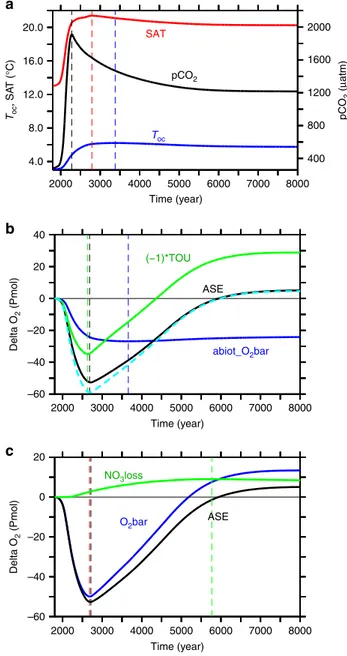
Our numerical model employing a business-as-usual emissions scenario with the emission peak in 2100 and a linear decline of emissions to zero in year 2300 (see“Methods”), simulates a rise in global-mean ocean temperatures by 3.1 °C above pre-industrial until year 3380 (Fig.1a). The associated solubility changes explain an oxygen decline by 27 Pmol (or 9%), as shown by the abiotic oxygen tracer (Fig.1b). This amounts to about half the simulated total oxygen loss at the time of the O2-inventory minimum (Fig.1c) and persists until the end of our experiment.
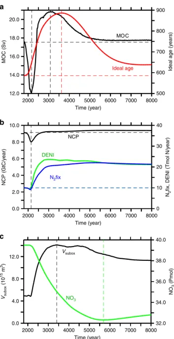
Changes in overturning. Consistent with earlier studies12,14–16, our model simulates an initial reduction in the meridional overturning circulation, which recovers after several centuries and reaches a maximum near year 3080 to eventually level off at an intensity slightly higher than preindustrial (Fig.2a). Explanations for such a recovery include a shift to enhanced deep-water for- mation in the southern hemisphere and an associated shoaling of the overturning circulation associated with North Atlantic Deep Water by about 1000 m. This shoaling also explains the increase in globally-averaged ideal age in spite of more vigorous over- turning (Fig. 2a). Ideal age increases by a few hundred years at mid-depth in the North Atlantic and Pacific Ocean (Fig.3c, d).
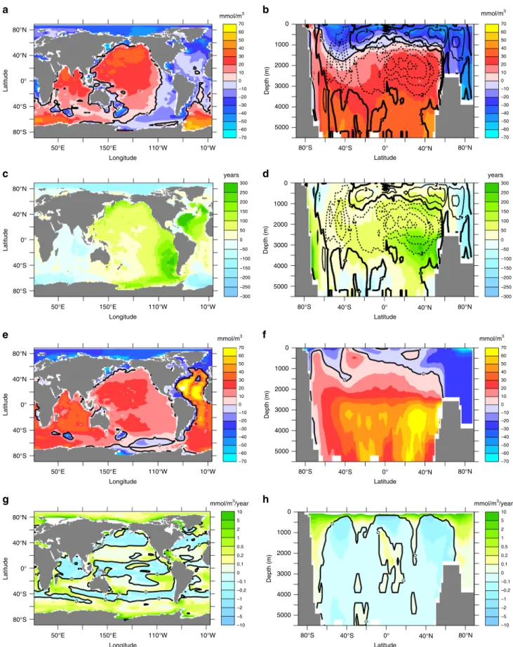
Changes in simulated oxygen in year 8000 relative to year 2000 reveal, on average, elevated oxygen concentrations below about 1000 m (Fig.3b), located mostly in the Southern Ocean and the Indo-Pacific region, whereas oxygen levels tend to decrease in the Atlantic and the Arctic Ocean (Fig.3a).
Changes in biological production. Net community production (NCP) describes the surplus of primary production over all
respiratory processes in the euphotic zone, which, on annual and longer time scales and global space scales corresponds to the organic matter exported from surface water. NCP initially declines by 12% until year 2145, then recovers, and eventually exceeds pre-industrial levels by about 3% (Fig.2b). The minimum in NCP occurs just when the strength of the meridional over- turning circulation is at its minimum (Fig. 2a). Once NCP increases again, the suboxic (O2< 5μM) volume starts to expand almost threefold within a few centuries (black curve, Fig. 2c).
Consequently, pelagic denitrification and, with a time lag of about 25 years, nitrogenfixation both increase and eventually level off at global rates about twice the pre-industrial rates (green and blue
O2bar
b a
c
abiot_O2bar
ASE NO3loss
(−1)*TOU ASE Toc
SAT
pCO2 20.0
16.0
Toc, SAT (°C)Delta O2 (Pmol)Delta O2 (Pmol) pCO2 (µatm)
12.0
8.0
4.0
40 20 0 –20 –40 –60
20
0
–20
–40
–60
2000 3000 4000 5000 Time (year)
6000 7000 8000
2000 3000 4000 5000 Time (year)
6000 7000 8000
2000 3000 4000 5000 Time (year)
6000 7000 8000 2000
1600
1200
800
400
Fig. 1Simulated temporal evolution of global indicators.aAtmospheric pCO2(black), global-mean surface air temperature (red) and global mean ocean temperature (blue);banomalies relative to pre-industrial of the global-mean of an abiotic oxygen tracer (blue), total oxygen utilisation (times−1, green), cumulative air-sea oxygen exchange (black; positive into the ocean) and the sum of abiotic tracer and total oxygen utilisation (dashed cyan); andcoxygen accumulation via nitrate loss (green), equivalent to the difference between global mean oxygen change (blue) and cumulative air-sea oxygenflux (black). Dashed vertical lines denote the time of maxima/minima of the respective curve of same colour
curves, Fig. 2b). At the end of the simulation, nitrogenfixation accounts for about 20% of the global NCP, compared to about 10% in year 2000.
Changes in respiratory oxygen consumption. At first sight, increases in global-mean ocean temperature (Fig. 1a), ideal age (Fig.2a) and NCP (Fig.2b) all suggest a declining global ocean oxygen inventory, as also put forward to explain past oceanic anoxic events17. The actually modelled oxygen increase (Fig.1c) can only arise from spatially inhomogeneous changes of tem- perature, ventilation, respiration, or other processes not yet considered. Indeed, changes in respiratory oxygen consumption via aerobic remineralisation of detritus show a systematic shift of enhanced export and subsequent remineralisation towards high latitudes (Fig.3g, h) linked to more efficient nutrient utilisation
via improved light conditions due to disappearing summer sea-ice and more stable stratification. Interestingly, particle export and subsequent remineralisation are also enhanced in the upper hundred metres of the subtropical gyres, while there is a general decline of respiration in less well ventilated deeper waters (Fig. 3h). In the model, this results from faster—and hence shallower—remineralisation at higher temperatures, leading to enhanced nutrient recycling in the upper ocean.
Accumulation of oxygen deficits. Although total respiration shows a slight increase, the oceanic storage of the respiratory oxygen deficit, measured here as true oxygen utilization (TOU18), is decreased considerably in the simulated future ocean. For the first few hundred years of our simulation, TOU increases ((−1)
*TOU decreases, green line in Fig. 1b). This is because of the longer residence time of upwelled waters in the more stratified surface waters allowing for a more complete biotic utilisation of surface nutrients, and elevated oxygen consumption during subsequent remineralisation in the ocean interior. TOU decreases ((−1)*TOU increases) after year 2630 and eventually the global TOU inventory becomes lower than the pre-industrial one. The total reduction in TOU amounts to an oxygen gain of 29 Pmol by the end of the simulation. This more than compensates the warming-driven oxygen loss from solubility changes of 24 Pmol, yielding a net oxygen surplus of 4.6 Pmol. This extra oxygen must enter the ocean via air-sea exchange. Indeed, the cumulative air-sea oxygen flux into the ocean by the end of the simulation (5.1 Pmol, Fig.1b, black line) very closely matches the combined oxygen loss via warming-induced solubility change and the oxygen gain by the decrease of TOU (Fig.1b, dashed cyan line).
Effects of nitrogen imbalances. The oxygen gained via air-sea gas exchange explains, however, only about one third of the total increase in the oceanic oxygen inventory (13.4 Pmol, i.e. 6% of today’s ocean O2inventory Fig.1c, blue line). Almost two thirds of it must therefore be from an oxygen source located in the ocean interior. Interior-ocean oxygen sources are photosynthesis, specifically, the net balance of oxygenic photosynthesis minus respiration, and processes reducing the oxidation state of nitrogen and other compounds. For everything else unchanged, a switch from aerobic to anaerobic respiration will cause a left-over of, and hence increase in, dissolved oxygen. Total marine oxygen may thus be saved by the utilization of an oxidant other than oxygen, like in denitrification, or it may be spent by oxidising an external source of reduced nitrogen, like in N2-fixation and subsequent nitrification of the newly added N. In our simulation the strong increase in pelagic denitrification together with the time-lagged increase in N2-fixation cause a net loss of the ocean’s fixed nitrogen (Fig.2c). Any net conversion, and loss, of nitrate to N2
via denitrification corresponds to a net gain of oxygen (Fig. 1c) because no oxygen is consumed in it. Anaerobic remineralization via denitrification of organic matter containing one mole of organic nitrogen avoids the consumption of 10.6 moles of oxygen while removing 7.48 moles of NO3(ref.19). Thus, for each mole of nitrate lost, about 1.4 moles of oxygen are gained. Deni- trification is hence an implicit source of oxygen to the ocean. The reverse applies to N2-fixation which is hence an oxygen sink for the ocean. What matters globally is the cumulative balance of denitrification and N2-fixation, that is the change in the global nitrate inventory. The total simulated nitrate loss of 6.2 Pmol NO3, i.e. about 17% of the present-day ocean’s nitrate inventory (green curve Fig.2c), corresponds to an oxygen gain of 8.8 Pmol O2 (Fig. 1c), which is about 4% of the present ocean oxygen inventory.
DENI
b a
MOC
NCP
c
N2fix
Vsubox
NO3
Ideal age 20.0
18.0
MOC (Sv)NCP (GtC/year)Vsubox (1015 m3) N2fix, DENI (Tmol N/year) NO3 (Pmol)Ideal age (years)
16.0
14.0
12.0
10.0
8.0
6.0
4.0
2.0
0.0
12.0
8.0
4.0
0.0
2000 3000 4000 5000 Time (year)
6000 7000 8000
2000 3000 4000 5000 Time (year)
6000 7000 8000
2000 3000 4000 5000 Time (year)
6000 7000 8000 900
800
700
600
500
40
30
20
10
0
40.0
38.0
36.0
34.0
32.0
Fig. 2Simulated temporal evolution of ocean state indicators.aMaximum of the meridional overturning stream function (black) and global average of ideal age (red);bglobal net community production (black), global denitrification (green), global nitrogenfixation (blue); andcsuboxic volume (black) and globally averaged nitrate concentrations (green)
c
a b
d
e
g h
f
mmol/m3
mmol/m3 mmol/m3
years years
mmol/m3
mmol/m3/year mmol/m3/year
80°N
0
1000
2000
Depth (m)
3000
4000
5000
0
1000
2000
Depth (m)
3000
4000
5000
0
1000
2000
Depth (m)
3000
4000
5000
0
1000
2000
Depth (m)
3000
4000
5000 40°N
LatitudeLatitudeLatitudeLatitude
0°
40°S
80°S
50°E 150°E
Longitude
110°W 10°W 80°S 40°S
Latitude
0° 40°N 80°N
80°S 40°S
Latitude
0° 40°N 80°N
80°S 40°S
Latitude
0° 40°N 80°N
80°S 40°S
Latitude
0° 40°N 80°N
70 60 50 40 30 20 10 0 –10 –20 –30 –40 –50 –60 –70
70 60 50 40 30 20 10 0 –10 –20 –30 –40 –50 –60 –70
70 60 50 40 30 20 10 0 –10 –20 –30 –40 –50 –60 –70
70 60 50 40 30 20 10 0 –10 –20 –30 –40 –50 –60 –70
10 5 2 1 0.5 0.2 0.1 0 –0.1 –0.2 –1 –2 –5 –10
10 5 2 1 0.5 0.2 0.1 0 –0.1 –0.2 –1 –2 –5 –10 300
250 200 150 100 50 0 –50 –100 –150 –200 –250 –300
300 250 200 150 100 50 0 –50 –100 –150 –200 –250 –300
50°E 150°E
Longitude
110°W 10°W
50°E 150°E
Longitude
110°W 10°W
50°E 150°E
Longitude
110°W 10°W
80°N
40°N
0°
40°S
80°S
80°N
40°N
0°
40°S
80°S
80°N
40°N
0°
40°S
80°S
Fig. 3Simulated ocean changes (year 8000 minus year 2000).a,bOxygen in mmol O2m−3;c,dideal age in years;e,ftotal oxygen utilisation in mmol O2m−3; andg,hremineralisation below 125 m in mmol O2m−3year−1. The left hand column (panelsa,c,e,g) shows vertically averaged changes, the right hand column shows zonally averaged changes. Contour lines in panelsbanddrefer to the zonally integrated meridional overturning stream function with transport in units Sv (106m3s−1)
Sulfate reduction to hydrogen sulfide, not considered in the model, would save still more oxygen in the water column.
However, unless outgassing to the atmosphere, hydrogen sulfide would most likely quickly be re-oxidised in the oxic waters surrounding the respective anoxic region, cancelling the initial oxygen gain. Not resolving the marine sulfur cycle, we cannot quantify to what extent the reaction of H2S with NO3, the formation of elemental sulfur, or the burial of FeS might modify this picture. Other processes that may affect oxygen, but are not explicitly accounted for in this model configuration, are burial and denitrification in the sediments as well as the release of sedimentary phosphate and iron under expanding oxygen- deficient regions20.
Nitrogenfixation feedback. The enhanced loss offixed nitrogen via denitrification can only lead to a sustained net decline in the ocean’s inventory offixed nitrogen, because nitrogenfixation only partly compensates the nitrogen loss. This, apparently, is contrary to the geochemical view that, on long timescales, nitrogen fixation feeds back on nitrogen losses and‘nitrate gets topped up when scarce relative to phosphate’ (ref. 21). In our simulation, nitrogen fixation is performed by diazotrophs with a maximum growth rate less than half of that of ordinary phytoplankton and zero growth at temperatures lower than 15 °C, but not limited by fixed nitrogen12. It starts to increase within 25 years after the onset of the rise in denitrification, but does so at a slower rate catching up with annual rates of nitrogen loss only well after year 5000 (Fig.2b). The initial delay is consistent with the time it takes for water to upwell from the oxygen minimum zones (with denitrification) to the surface22. Simulated global nitrogenfixa- tion more than doubles within a few hundred years (Fig. 2b). It
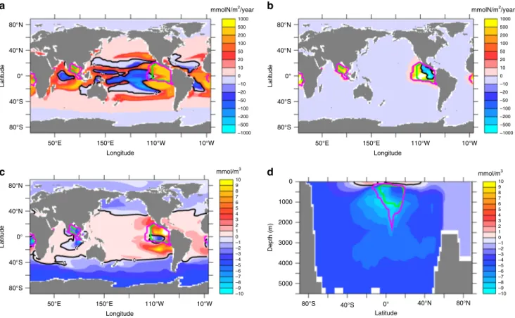
expands its range with the poleward migration of the 15 °C iso- therm (Fig. 4a). Areas of enhanced denitrification, however, remain located in the tropical oceans (Fig. 4b). As shown in Figs. 4c, d, lowest values of N*=NO3–16 PO4 (ref. 23,24) that measures the nitrate excess relative to the stoichiometric equivalent of phosphate, are simulated in regions of ongoing denitrification in the tropical oceans, whereas positive N* values are found in the surface waters of the tropical and subtropical oceans, roughly coinciding with areas of nitrogen fixation (Fig. 4a). Surface waters at high latitudes, particularly in the Southern Ocean, and almost all of the deep ocean waters, how- ever, display negative N* values. This illustrates that part of the denitrification signature is upwelled in the Southern Ocean, where high nutrient levels and low surface temperatures and light levels do not present favourable conditions for nitrogenfixation.
Deep-water formation south of the Southern Ocean biogeo- chemical divide25ensures that any upwelled low-N* waters can be transported into the deep ocean without supporting nitrogen fixation. It thereby acts as a loophole through which denitrification-induced nitrogen deficits can escape the surface- ocean nitrogen-fixation feedback and preserve significant oceanic nitrate deficits in the ocean interior.
Decoupling of biological production and nutrient inventory.
An interestingfinding is that global NCP is essentially unchanged and even shows a slight increase (Fig.2b) despite a 17% decline in the ocean’s nitrate inventory (Fig.2c). This decoupling of global NCP and nutrient inventory can be explained by the spatial pattern of the accumulated nitrate deficit, which very closely corresponds to the pattern of N* (Fig.4c, d): Nitrate concentra- tions are lowered predominantly in the deep ocean and in
a b
mmol/m3 mmol/m3
c d
mmolN/m2/year mmolN/m2/year
80°N
1000 500 200 100 50 20 10 0 –10 –20 –50 –100 –200 –500 –1000
10 9 8 7 6 5 4 3 2 1 0 –1 –2 –3 –4 –5 –6 –7 –8 –9 –10
10 9 8 7 6 5 4 3 2 1 0 –1 –2 –3 –4 –5 –6 –7 –8 –9 –10
1000 500 200 100 50 20 10 0 –10 –20 –50 –100 –200 –500 –1000
40°N
0 0
0
0
0
0 0
0°
40°S
80°S
50°E 150°E 110°W 10°W
Latitude
80°N
40°N
0°
40°S
80°S
0
1000
2000
3000
4000
5000
LatitudeDepth (m)
80°N
40°N
0°
40°S
80°S
Latitude
Longitude
50°E 150°E 110°W 10°W 80°S 40°S 0° 40°N 80°N
Longitude
50°E 150°E 110°W 10°W
Longitude
Latitude
Fig. 4Simulated nitrogen-cycle changes (year 8000 minus year 2000).aAnnual mean vertically integrated nitrogenfixation,bannual mean vertically integrated denitrification,csurface concentrations in N*=NO3–16 PO4, anddzonally averaged N*. Green contours refer to the maximum extent of suboxic waters (O2< 5μM) in year 2000, magenta contours to the maximum extent of suboxic waters in year 8000
high-latitude surface waters, whereas nitrate concentrations do not change significantly or even increase in the tropical and subtropical surface layers where phytoplankton growth is typi- cally limited by nitrogen26.
Discussion
Our modelling study of global-warming effects over millennia suggests expanding ocean anoxia (and the associated switch from aerobic respiration to denitrification) to eventually result in a counterintuitive net increase of marine oxygen levels. For each mole nitrate consumed via denitrification, about 1.4 moles of O2
are saved. The same amount of oxygen is consumed when organic nitrogen stemming from nitrogenfixation is oxidised to nitrate.
For a net oxygen gain it is essential that the commonly assumed feedback between nitrogen fixation and denitrification operates only with a temporal lag. The imbalance between nitrogenfixa- tion and denitrification lasts for about 3000 years in our model simulation (Fig.2b). In our model this is by the entrainment of nitrate-deficient waters into deep-water formation regions, par- ticularly in the Southern Ocean. Via this loophole, nitrate deficits can escape the topping-up action of nitrogenfixation and instead remain stored in the deep ocean, effecting a net oxygen gain. A major uncertainty (and on the agenda for future research) are the environmental controls of nitrogen fixation. Sensitivity experi- ments performed with a mechanistically different model of nitrogen fixation that includes the ability to access dissolved organic phosphorus and also allows diazotrophs to grow at low temperatures27, yield similar results regarding the temporal lag of the nitrogenfixation, but with only about half the simulated total loss of nitrate and associated gain of oxygen. If current assumptions about the environmental controls of nitrogen fixa- tion are correct and properties of deep ocean waters can be set relatively unaffected by nitrogen fixation, the process modelled here leading to a net oceanic oxygen gain for a long-term global warming scenario may well have operated also during the development of whole-ocean anoxic events, e.g. in the Cretaceous.
It seems to be more difficult to develop marine anoxia than thought until now.
Methods
Model configuration. The model used is the University of Victoria (UVic) Earth System Climate Model28in the configuration described by ref.12. The ocean component is a fully three-dimensional primitive-equation model with nineteen levels in the vertical ranging from 50 m near the surface to 500 m in the deep. It contains a simple marine ecosystem model including the two major nutrients nitrate and phosphate and two phytoplankton classes, nitrogenfixers and other phytoplankton, the former being limited by phosphate only. As a caveat we note that the micronutrient iron is not explicitly included in the model, which never- theless achieves a reasonablefit to observed biogeochemical tracer distributions for the tuned biological parameters and mixing parameterizations12,29. For the molar stoichiometry of C:N:P:−O2=112:16:1:169.6 assumed in the model19, organic matter is degraded by aerobic remineralisation (−O2:PO4=169.6) as long as sufficient dissolved oxygen is available. In regions where oxygen concentrations are below a threshold of 5 mmol O2m−3, nitrate is used as electron acceptor (deni- trification,−NO3:PO4=119.68). No other electron acceptors are simulated and remineralisation stops whenever nitrate runs out, which happens only occasionally at very few grid points. A suite of idealised tracers is added comprising ideal age30, an abiotic oxygen tracer affected only by air-sea gas exchange and surface-water solubility31, and a tracer of preformed PO4that is, at every model time step, set identical to the model’s PO4tracer in the surface layer, but otherwise a passive tracer without sinks or sources32. TOU is computed as the stoichiometric oxygen equivalent of regenerated PO4, i.e. total PO4minus preformed PO4.
The ocean component is coupled to a single-level energy-moisture balance model of the atmosphere and a dynamic-thermodynamic sea ice component and a terrestrial vegetation and carbon-cycle component28. All model components use a common horizontal resolution of 1.8° latitude times 3.6° longitude. The current model version does not consider anyfluxes across the water-sediment interface and also does not account forfluxes related to weathering on land. Oceanic phosphorus is thus strictly conserved. Because the atmosphere contains about a hundred times as much oxygen as the ocean, any feedback of marine oxygen changes on atmospheric oxygen is neglected as in earlier studies (e.g. ref.11).
Global warming scenario. After a spin-up of more than 10,000 years under pre- industrial atmospheric and astronomical boundary conditions, the model is run under historical conditions from year 1850 to 2000 using fossil-fuel and land-use carbon emissions as well as solar, volcanic and anthropogenic aerosol forcings.
From year 2000 to 2100, the model is forced by CO2emissions following the Special Report on Emissions A2 non-intervention scenario33reaching maximum emissions of about 29 PgC/year in the year 2100. Thereafter, CO2emissions decrease linearly to zero in year 2300. In this simulation, 2200 GtC are emitted until year 2100 and a total of 5100 GtC until year 2300. Model simulations are continued with zero CO2emissions after year 2300 until year 8000.
Data availability
Model results generated as part of this study are available athttps://data.geomar.de/
thredds/catalog/open_access/oschlies_et_al_2019_nc/catalog.html
Code availability
All code used to generate the results of this study is available athttps://data.geomar.de/
thredds/catalog/open_access/oschlies_et_al_2019_nc/catalog.html
Received: 18 September 2018 Accepted: 4 June 2019
References
1. Keeling, R. F., Körtzinger, A. & Gruber, N. Ocean deoxygenation in a warming world.Annu. Rev. Mar. Sci.2, 199–229 (2010).
2. Gruber, N. Warming up, turning sour, losing breath: Ocean biogeochemistry under global change.Philos. Trans. Roy. Soc. A369, 1980–1996 (2011).
3. Breitburg, D. et al. Declining oxygen in the global ocean and coastal waters.
Science359,https://doi.org/10.1126/science.aam7240(2018).
4. Oschlies, A., Brandt, P., Stramma, L. & Schmidtko, S. Drivers and mechanisms of ocean deoxygenation.Nat. Geosci.11, 467–473 (2018).
5. Stramma, L., Johnson, G. C., Sprintall, J. & Mohrholz, V. Expanding oxygen- minimum zones in the tropical oceans.Science320, 655–658 (2008).
6. Helm, K. P., Bindoff, N. L. & Church, J. A. Observed decreases in oxygen content of the global ocean.Geophys. Res. Lett.38, L23602 (2011).
7. Schmidtko, S., Stramma, L. & Visbeck, M. Decline in global oceanic oxygen content during the pastfive decades.Nature542, 335–339 (2017).
8. Watson, A. J., Lenton, T. M. & Mills, B. J. W. Ocean deoxygenation, the global phosphorus cycle and the possibility of human-caused large-scale ocean anoxia.Philos. Trans. Roy. Soc. A375, 20160318 (2017).
9. Jenkyns, H. C. Geochemistry of oceanic anoxic events.Geochem. Geophys.
Geosyst.11, Q03004 (2010).
10. Bopp, L. et al. Multiple stressors of ocean ecosystems in the 21stcentury:
projections with CMIP5 models.Biogeosciences10, 6225–6245 (2013).
11. Shaffer, G., Olsen, S. M. & Pedersen, J. O. P. Long-term ocean oxygen depletion in response to carbon dioxide emissions from fossil fuels.Nat.
Geosci.2, 105–109 (2009).
12. Schmittner, A., Oschlies, A., Matthews, H. D. & Galbraith, E. D. Future changes in climate, ocean circulation, ecosystems, and biogeochemical cycling simulated for a business-as-usual CO2emission scenario until year 4000 AD.
Glob. Biogeochem. Cycles22, GB1013 (2008).
13. Ridgwell, A. & Schmidt, D. N. Past constraints on the vulnerability of marine calcifiers to massive carbon dioxide release.Nat. Geosci.3, 196–200 (2010).
14. Yamamoto, A. et al. Global deep ocean oxygenation by enhanced ventilation in the Southern Ocean under long-term global warming.Glob. Biogeochem.
Cycles29, 1801–1815 (2015).
15. Matear, R. J. & Hirst, A. C. Long-term changes in dissolved oxygen concentrations in the ocean caused by protracted global warming.Glob.
Biogeochem. Cycles17, 4 (2003).
16. Zickfeld, K. et al. Long-term climate change commitment and reversibility: an EMIC intercomparison.J. Clim.26, 5782–5809 (2013).
17. Ozaki, K., Tajima, S. & Tajika, E. Conditions required for oceanic anoxia/
euxinia: Constraints from a one-dimensional ocean biogeochemical cycle model.Earth Planet. Sci. Lett.304, 270–279 (2011).
18. Ito, T., Follows, M. J. & Boyle, E. A. Is AOU a good measure of respiration in the oceans?Geophys. Res. Lett.31, L17305 (2004).
19. Paulmier, A., Kriest, I. & Oschlies, A. Stoichiometries of remineralisation and denitrification in global biogeochemical ocean models.Biogeosciences6, 923–935 (2009).
20. Niemeyer, D., Kemena, T. P., Meissner, K. J. & Oschlies, A. A model study of warming-induced phosphorus–oxygen feedbacks in open-ocean oxygen minimum zones on millennial timescales.Earth Syst. Dyn.8, 357–367 (2017).
21. Tyrrell, T. The relative influences of nitrogen and phosphorus on oceanic primary production.Nature400, 525–531 (1999).
22. Glessmer, M. S., Park, W. & Oschlies, A. Simulated reduction in upwelling of tropical oxygen minimum waters in a warmer climate.Environm. Res. Lett.6 https://doi.org/10.1088/1748-9326/6/4/045001(2011).
23. Michaels, A. F. et al. Inputs, losses and transformations of nitrogen and phosphorus in the pelagic North Atlantic Ocean.Biogeochemistry35, 181–226 (1996).
24. Gruber, N. & Sarmiento, J. L. Global patterns of marine nitrogenfixation and denitrification.Glob. Biogeochem. Cycles11, 235–266 (1997).
25. Marinov, I., Gnanadesikan, A., Toggweiler, J. & Sarmiento, J. The Southern Ocean biogeochemical divide.Nature441, 964–967 (2006).
26. Moore, C. M. et al. Processes and patterns of oceanic nutrient limitation.Nat.
Geosci.6, 701–710 (2013).
27. Landolfi, A., Koeve, W., Dietze, H., Kähler, P. & Oschlies, A. A new perspective on environmental controls of marine nitrogenfixation.Geophys.
Res. Lett.42, 4482–4489 (2015).
28. Weaver, A. J. et al. The UVic earth system climate model: model description, climatology, and applications to past, present and future climates.
Atmosphere-Ocean39, 361–428 (2001).
29. Oschlies, A., Schulz, K. G., Riebesell, U. & Schmittner, A. Simulated 21st century’s increase in oceanic suboxia by CO2-enhanced biological carbon export.Glob. Biogeochem. Cycles22, GB4008 (2008).
30. England, M. H. The age of water and ventilation timescales in a global ocean model.J. Phys. Oceanogr.25, 2756–2777 (2015).
31. Dietze, H. & Oschlies, A. On the correlation between air-sea heatflux and abiotically induced oxygen gas exchange in a circulation model of the North Atlantic.J. Geophys. Res.110, C09016 (2005).
32. Ito, T. & Follows, M. J. Preformed phosphate, soft tissue pump and atmospheric CO2.J. Mar. Res.63, 813–839 (2005).
33. Nakicenovic, N. et al.Special Report on Emissions Scenarios (SRES), A Special Report of Working Group III of the Intergovernmental Panel on Climate Change. (Cambridge University Press, Cambridge, 2000).
Acknowledgements
This work was supported by the German Research Foundation (DFG) as part of the research project SFB 754‘Climate-Biogeochemistry Interactions in the Tropical Ocean’.
Author contributions
All authors discussed the results and wrote the manuscript. A.O. designed the study, performed the simulations and led the analysis and writing. W.K., A.L. and P.K. con- tributed to analysis, interpretation of results and writing.
Additional information
Supplementary Informationaccompanies this paper athttps://doi.org/10.1038/s41467- 019-10813-w.
Competing interests:The authors declare no competing interests.
Reprints and permissioninformation is available online athttp://npg.nature.com/
reprintsandpermissions/
Peer review information:Nature Communicationswould like to thank Richard Matear and other anonymous reviewers for their contributions to the peer review of this work.
Peer review reports are available.
Publisher’s note:Springer Nature remains neutral with regard to jurisdictional claims in published maps and institutional affiliations.
Open Access This article is licensed under a Creative Commons Attribution 4.0 International License, which permits use, sharing, adaptation, distribution and reproduction in any medium or format, as long as you give appropriate credit to the original author(s) and the source, provide a link to the Creative Commons license, and indicate if changes were made. The images or other third party material in this article are included in the article’s Creative Commons license, unless indicated otherwise in a credit line to the material. If material is not included in the article’s Creative Commons license and your intended use is not permitted by statutory regulation or exceeds the permitted use, you will need to obtain permission directly from the copyright holder. To view a copy of this license, visithttp://creativecommons.org/
licenses/by/4.0/.
© The Author(s) 2019