A dynamical reconstruction of the global monthly-mean oxygen isotopic composition of seawater

A dynamical reconstruction of the global

monthly-mean oxygen isotopic composition of seawater

Charlotte Breitkreuz¹, Andr´e Paul¹, Takasumi Kurahashi-Nakamura¹, Martin Losch², Michael Schulz¹

C. Breitkreuz, cbreitkreuz@marum.de

1MARUM - Center for Marine Environmental Sciences and Faculty of Geosciences, University of Bremen, Bremen, Germany

2AWI - Alfred-Wegener-Institut, Helmholtz Zentrum f¨ur Polar- und

Meeresforschung, Bremerhaven, Germany

This article has been accepted for publication and undergone full peer review but has not been through the copyediting, typesetting, pagination and proofreading process, which may lead to differences

Abstract. We present a dynamically consistent gridded data set of the global, monthly-mean oxygen isotope ratio of seawater (δ¹⁸O_sw). The data set was created from an optimized simulation of an ocean general circula- tion model constrained by global monthly δ¹⁸O_sw data collected from 1950 until 2011 and climatological salinity and temperature data collected from 1951 to 1980. The optimization was obtained using the adjoint method for variational data assimilation, which yields a simulation that is consistent with the observational data and the physical laws embedded in the model. Our data set performs equally well as a previous data set in terms of model-data misfit but brings an improvement in terms of the seasonal cycle and phys- ical consistency. As a result the data set does not show any sharp transitions between water masses or in areas where the data coverage is low. The data assimilation method shows high potential for interpolating sparse data sets in a physically meaningful way. Comparatively big errors, however, are found in our data set in the surface levels in the Arctic Ocean mainly because the influence of isotopically highly depleted precipitation is not preserved in the sea-ice model, and the low model resolution of about 285 km horizontally.

The data set is publicly available and it is anticipated to be useful for a large range of applications in (paleo-) oceanographic studies.

Keypoints:

• Physically consistent data set of the global, 3-dimensional oxygen iso- topic distribution of the ocean

• Using the adjoint method to fit an ocean general circulation model to observational data

• Data set available for potential applications in (paleo-)oceanography

Plain Language Summary

The ratio of the heavier to the lighter oxygen isotope in seawater varies over different areas and for different water masses in the ocean. In this study we present a global gridded data set of the monthly-mean oxygen isotope ratio of seawater (δ¹⁸O_sw). The data set is publicly available and will be useful for a large range of applications. It can, for example, help to reconstruct past ocean states, or be used as lower boundary for an atmospheric model to investigate the isotopic composition of the atmosphere. The data set is taken from a simulation of a numerical ocean model that is in consistency with global δ¹⁸O_sw observations collected from 1950 until 2011 and monthly salinity and temperature observations collected from 1951 to 1980. To obtain the model simulation, we used a data assimilation method that brings the model simulation into consistency with the observational data. The ocean model is based on physical laws and therefore, our data set is also in consistency with the ocean physics. Our data set is similarly close to the observations than a previous data set, but brings an improvement because it is based on the ocean physics and because it has a seasonal cycle.

1. Introduction

The oxygen isotopic ratio of water, expressed as δ¹⁸O = _R^18O/16O

VSMOW −1·1000‰ with respect to the Vienna Standard Mean Ocean Water [VSMOW, R_VSMOV = 2005.2·10⁻⁶, Gonfiantini, 1978], is a tracer of the Earth’s hydrological cycle. It depends on the origin and composition of the respective water [Craig and Gordon, 1965; Gat, 1996] and can be used, for example, as indicator of sea-ice melt, continental and glacial run-off, or as tracer of ocean water masses [e.g. Jacobs et al., 1985; Khatiwala et al., 1999; Meredith et al., 1999a;Macdonald et al., 1999;Paul et al., 1999].

Additionally,δ¹⁸O is one of the most abundant proxies for the past climate as its signal is stored in a wide range of climate archives. The oxygen isotopic ratio of precipitation, for example, is preserved in continental ice or in speleothem records. In the ocean the oxygen isotopic composition of seawater (δ¹⁸O_sw) is preserved in the shells of calcareous organisms such as planktonic and benthic foraminifera. The isotopic composition of their calcite shells (δ¹⁸O_c) depends not only on the isotopic composition of ambient seawater but also on its temperature [McCrea, 1950]. The signal stored in the shells can be used to reconstruct past temperature [e.g. Emiliani, 1955] or δ¹⁸O_sw [e.g. Duplessy et al., 1991]. Modern data sets are important for the calibration of the relationship between δ¹⁸O_sw, δ¹⁸O_c and temperature in cases where in-situ measurements ofδ¹⁸O_sw are not available [e.g.,Mulitza et al., 2003], for the comparison with past climate δ¹⁸O_sw or δ¹⁸O_c reconstructions [e.g., Lund et al., 2011], or for the calibration of other proxies [e.g., Groeneveld and Chiessi, 2011].

A 3-dimensional gridded data set of δ¹⁸Osw was presented by LeGrande and Schmidt [2006]. It is based on interpolating a large set of observationalδ¹⁸O_sw data using regional linear relationships between δ¹⁸O_sw and salinity evaluated for distinct regions and water masses. This data set was used frequently, for example, as surface boundary condition for an isotope-enable atmospheric model [e.g. Werner et al., 2011] or for the calibration of proxies [e.g. Mathien-Blard and Bassinot, 2009; Cleroux et al., 2008; Groeneveld and Chiessi, 2011].

Here, we present a new global, 3-dimensional gridded data set ofδ¹⁸O_sw that introduces two major improvements. First, it includes a seasonal cycle and second, it is physically consistent, that is, consistent with the physical laws implemented in an ocean general

circulation model. The data set is based on an optimized 400-year quasi-equilibrated sim- ulation of a water isotope-enabled global ocean general circulation model. The simulation is obtained using the adjoint method for variational data assimilation and consistent with monthly salinity, temperature andδ¹⁸O_sw data within their respective uncertainties.

The adjoint method has recently been used to obtain a long (400-year) optimized simu- lation of the modern and the Last Glacial Maximum (19-23 ka BP) ocean and its oxygen isotopic composition below 150 m water depth [Kurahashi-Nakamura et al., 2017]. We ex- tend their optimization in two ways. First, we use a general circulation model enhanced with a water isotope module that allows us to simulate water isotopes at the surface as well as in the deep ocean. Second, we introduce an adjustment to their technique to obtain a quasi-equilibrated simulation.

2. Material and Methods 2.1. Model

We used the Massachussets Institute of Technology general circulation model (MIT- gcm) in a configuration that solves the Boussinesq form of the hydrostatic Navier-Stokes equations [Marshall et al., 1997; MITgcm Group, 2016]. The model uses a cubed-sphere grid [Ronchi et al., 1996] with 192 × 32 horizontal grid cells encompassing the global ocean, resulting in a horizontal resolution of about 285 km, and 15 vertical levels with a resolution of 50 m at the surface to 690 m in the deepest level reaching a maximum depth of 5200 m. The vertical resolution of 50 m at the surface was chosen because it is the minimum value necessary to represent the mixed layer and to resolve the seasonal cycle. The cubed-sphere grid avoids converging grid cells at the poles and, hence, polar singularities. The boundary conditions at the ocean surface are prescribed as monthly at-

mospheric forcing, namely air temperature, meridional and zonal wind velocities, specific humidity, precipitation, downward short- and longwave radiation and river run-off, based on the Coordinated Ocean-ice Reference Experiments [COREs,Griffies et al., 2009]. Bulk formulae are used to compute outgoing radiation, wind stress and evaporation [Large and Yeager, 2004]. The ocean model is fully coupled to a dynamic-thermodynamic sea-ice model [Losch et al., 2010], which uses the same grid and the same atmospheric forcing.

Subgrid-scale mixing is parameterized with a GM/Redi scheme [Gent and Mcwilliams, 1990]. Due to the low resolution of the model some physical processes, such as the coastal and equatorial upwelling or the western boundary currents, are poorly resolved. The low computational cost, however, allows us to obtain a long optimized simulation with the adjoint method in a reasonable amount of time.

The MITgcm is extended with a water isotope module that comprises the fractionation processes of water isotopes during evaporation over the ocean and allows the model to simulate stable water isotopes in the entire water column [V¨olpel et al., 2017]. The module does not include the simulation of the isotopic composition of sea-ice and therefore, the isotopic composition of precipitation does not affect the seawater in areas with sea-ice.

In this study the concentration of the stable isotopes H¹⁶₂ O and H¹⁸₂ O are included in the simulation such that the δ¹⁸O_sw distribution can be computed. The climatological monthly isotopic composition of precipitation and water vapor were obtained from a water isotope-enabled simulation with the Community Atmosphere Model version 3.0 [IsoCAM3.0, Tharammal et al., 2013] and are prescribed as boundary conditions for the water isotope module. The prescribed isotopic composition of precipitation was previously used byV¨olpel et al.[2017], who compared it to observations from the Global Network of

Isotopes in Precipitation (GNIP) and found a good agreement. The isotopic composition of river run-off is defined in the model by the isotopic composition of precipitation at the location of the river mouth because the model does not explicitly simulate the isotopic composition of precipitation over river catchment areas [V¨olpel et al., 2017].

One main advantage of the MITgcm model code is that it is tailored to automatic differ- entiation [Griewank and Walther, 2008]. This allows generating the adjoint of the MIT- gcm model code with a source-to-source translator [Giering, 2000;Giering and Kaminski, 1998] and, hence, applying the adjoint method. We adjusted the model code of the newly added water isotope module [V¨olpel et al., 2017] to make it suitable for the generation of the adjoint code.

2.2. Observational Data and Uncertainties

To constrain our simulation we assimilated climatological temperature and salinity data that were previously prepared by Kurahashi-Nakamura et al. [2017]. They computed monthly means from daily data from 1951 to 1980 from the World Ocean Atlas database [Antonov et al., 2010;Locarnini et al., 2010]. The respective uncertainties were computed from the standard deviation within the data set. An additional uncertainty of 1 K for tem- perature and 0.1for salinity were added to account for data representativeness and model error. Kurahashi-Nakamura et al. [2017] excluded data in the equatorial and coastal up- welling areas, enclosed basins such as the Mediterranean, and the Arctic Ocean from their data set (their Fig. A1). In these areas the model has a strong bias due to the low model resolution andKurahashi-Nakamura et al.[2017] found that unphysical adjustments of the control variables would have been necessary to fit the model to the data in these regions.

As we are using the same model grid we inherit the same changes in the temperature and salinity data sets.

The simulated oxygen isotopic distribution is constrained by observational δ¹⁸O_sw data from the NASA GISS Global Seawater Oxygen-18 Database [version 1.21, https://data.giss.nasa.gov/o18data/,Schmidt et al., 1999]. This data set, which was also the basis of the data set byLeGrande and Schmidt [2006], contains more than 22,000 data points collected from 1950 until 2011. We modified the data as suggested by LeGrande and Schmidt [2006], excluding data that were partly read off a graph, highly anomalous data, and data representing estuarine or river water or that were highly influenced by melt water. Additionally, we excluded data that are not on our model grid, such as data from the Baltic and the Black Seas and other single data points in the Canadian archipelago for which no ocean grid cell was found within a radius of 300 km.

Monthly variations are taken into account and data points for which this time informa- tion was not available were not used. After this quality control 19,683 valid data points remained. The data were averaged onto our model grid. Whenever more than one data point within a single grid cell for the same month was found we applied an inverse-distance weighting using the vertical distance to the center of the grid cell. In this way, data val- ues were assigned to 4305 grid cells, which corresponds to 0.6 % of the simulated global monthly-varying ocean. The uncertainties of the δ¹⁸O_sw data used in the cost function are an estimate of the sum of the uncertainties that determine how well the model can represent the data. These uncertainties include the measurement error of about 0.08‰ [Gat and Gonfiantini, 1981], time variations inδ¹⁸O_sw within one month, representative- ness uncertainties and model errors. We assume the sum of those errors to be spatially

uniform with a value of 0.2‰ as suggested by Kurahashi-Nakamura et al. [2017] except for the regions where temperature and salinity data had been removed. For these data points we set the uncertainty to 0.4‰ to compensate for the comparatively large model errors in these regions.

2.3. Optimization

The adjoint method [Errico, 1997; Wunsch, 1996] is used to minimize a cost function that measures the model-data misfit in a least-squares sense. The minimization is achieved by adjusting defined control variables, for example, initial or boundary conditions or internal model parameters. A successful minimization of the cost function with the adjoint method yields an estimate that is consistent with the model physics, as well as with the data within their uncertainties as prescribed in the cost function. The method is based on the “adjoint” model code, which computes the gradient of the cost function with respect to the control variables. This gradient is used to adjust the control variables with an iterative quasi-Newton descent algorithm [Nocedal, 1980; Gilbert and Lemar´echal, 1989]

to reduce the cost function. The adjoint code is obtained by applying a source-to-source transformation tool [Giering and Kaminski, 1998].

Experimental Design

The optimization was realized in two phases. In the first phase the model was fit to the temperature and salinity climatologies. An accurate simulation of these physical tracers is essential to achieve a realistic simulation of the ocean circulation and, hence, for an accurate simulation of water isotopes. In this first phase we did not include δ¹⁸O_sw data as we assumed that the temperature and salinity data sufficiently constrain the circulation.

Subsequently, in the second phase, the model was fit to theδ¹⁸O_sw data by adjusting only

the isotopic composition of precipitation and of water vapor and the initial conditions of the isotopic tracers. The δ¹⁸O_sw data, therefore, do not constrain the ocean general circulation but only the simulated isotopic composition.

For a non-linear optimization to be successful, it is essential to start from a good first guess of the control variables. Due to the tangent linear character of the adjoint method, the longer the model run the more difficult it is to obtain a good reduction of the cost function. Here, we aimed for a 400-year long optimized simulation such that the signal from the adjusted control variables can be transported from the surface to the deep ocean.

Even though 400 years are not enough to fully equilibrate the deep ocean [Wunsch and Heimbach, 2008], it was not possible to obtain a longer optimized simulation due to the substantial computational cost. A typical simulation obtained from the adjoint method with an ocean general circulation model spans 10 - 50 years [e.g.Forget et al., 2015; K¨ohl et al., 2007; K¨ohl and Stammer, 2008]. To achieve the comparatively long optimized 400- year run we adopted a ”carry-over” technique [Dail, 2012; Kurahashi-Nakamura et al., 2017]. We started with an optimization of a 20-year run and in a sequence, the optimized control variables from the shorter run are used as a starting point in the optimization of a longer run, eventually reaching the desired length. This technique imposes a substantial amount of computational cost but it is to our knowledge as yet the only way to obtain a 400-year optimized simulation with the adjoint method.

Phase 1

To create initial conditions for the optimization the model was spun-up for 4000-years with the original first-guess control variables. For the first phase, following Kurahashi- Nakamura et al. [2017], we chose the atmospheric forcing fields (i.e., air temperature,

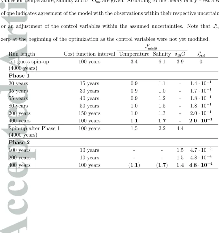
specific humidity, precipitation, zonal and meridional wind velocities, downward short- wave and longwave radiation), the initial conditions for the physical tracers (salinity, temperature) and the spatially-varying vertical diffusivity as control variables. The opti- mization with the carry-over technique was started with a 20-year long run followed by a 35-, a 50-, an 80-, a 200- and finally a 400-year run. The cost function was computed for a certain time interval at the end of each run. The carry-over intervals and the length of the respective cost function interval (Table 1) were chosen such that they were not multiples of one another to avoid an oscillation in the optimized simulation reflecting the length of the carry-over intervals. We discovered such an oscillation in the optimized modern simulation by Kurahashi-Nakamura et al.[2017].

The cost function in this phase consists of the three terms J₁ = J_misfit1 +J_ctrl1 +J_eq. The first term J_misfit1 quantifies the misfit between model and data. It has the form

Jmisfit1 = (Smod −Sobs)^> WS (Smod−Sobs) + (Tmod−Tobs)^> WT (Tmod−Tobs). (1) Here, S_mod, S_obs, T_mod andT_obs are vectors containing temperature and salinity, modeled and observed values, respectively. The modeled values are long-term monthly means at the observed grid cells. The length of the interval over which the mean is calculated depends on the respective step in the carry-over phase. The weighting matrices W_S,T are the inverse of the error-covariance matrices of the respective data. We assumed the uncertainties of the data to be spatially uncorrelated such that the matrices are diagonal.

The second term of the cost function J_ctrl1 penalizes the adjustments of the control variables. These penalty terms ensure that the optimized control variables do not depart too much from their first guess values. Mathematically speaking the optimization without these penalty terms is a highly under-determined problem, that is, the number of control

variables is much higher than the number of model-data comparisons in Jmisfit and the penalty terms serve to regularize the problem. Note that, for example, air temperature alone corresponds to 192× 32 grid cells times 12 months = 73728 control variables.

According to the control variables this part of the cost function is given by

J_ctrl1 = T₀^orig−T₀^mod> W_T0 T₀^orig−T₀^mod +S₀^orig−S₀^mod> W_S0 S₀^orig−S₀^mod +

7

X

i=1

F_i^orig−F_i^mod> WFi

F_i^orig−F_i^mod

+K^orig−K^mod> W_K K^orig−K^mod. (2)

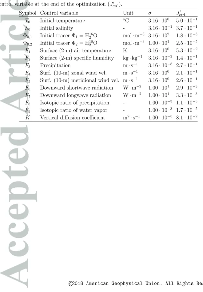
Each term represents the penalty on the deviation of the modified (mod) from the first guess (orig) control variables. The weighting matrices W are, as before, the inverse of the diagonal error covariance matrix of the respective first guess control variables. An explanation for the different symbols (i.e., different control variables), and the assumed standard deviations for the respective control variables can be found in Table 2.

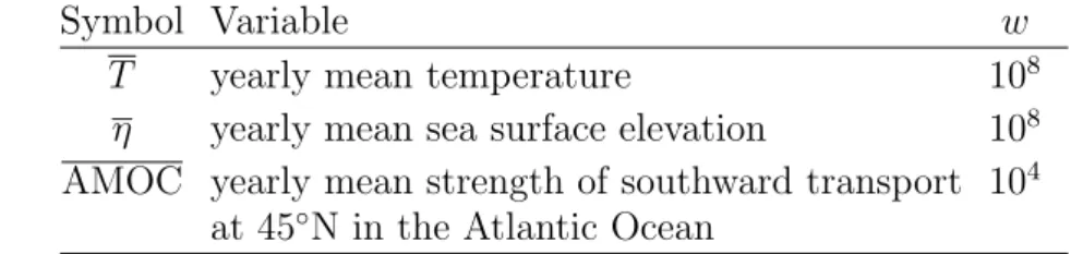
The third term of the cost function J_eq =w_T

tend−1

X

t=1

(T_t−T_t+1)²+w_η

tend−1

X

t=1

(η_t−η_t+1)²+w_AMOC

tend−1

X

t=1

(AMOC_t−AMOC_t+1)² (3) forces the model to obtain a stable, equilibrated ocean circulation. It penalizes drift in the yearly mean temperature (T), yearly mean global sea surface elevation (η) and the Atlantic Meridional Overturning Circulation (AMOC) measured by the yearly mean strength of the southward transport at 45^◦N in the Atlantic Ocean (AMOC) between each year (1, .., t_end) in the respective cost function interval. The respective weighting factors

w_{T , η, AMOC} (Table 3) were determined empirically such that the penalty restrained the drift but did not interfere too much with the reduction of J_misfit1.

Phase 2

To generate initial conditions for the isotopic tracers the model was spun-up for 4000 years with the optimized controls from Phase 1 starting from a spatially constant isotopic distribution. Subsequently, the optimization started with a 100-year run using the pre- viously optimized controls, carried-over to the optimization of a 200- and subsequently a 400-year run. In Phase 2 an oscillation cannot develop because the optimized physical controls from Phase 1 were held fixed, that is, no further adjustments were made to the previous controls in Phase 2. The model was fit to the δ¹⁸O_sw data by adjusting the isotopic ratios in precipitation and water vapor, and the initial conditions of the isotopic tracers H¹⁶₂ O and H¹⁸₂ O. The cost function consists of the two terms

J2 = Jmisfit2 +Jctrl2

= δ¹⁸O_mod−δ¹⁸O_obs^> W_δ¹⁸_O δ¹⁸O_mod−δ¹⁸O_obs (4)

+ ^X

i=1,2

Φ^orig_0,i −Φ^mod_0,i ^> W_Φ0,i Φ^orig_0,i −Φ^mod_0,i (5)

+ ^X

i=8,9

F_i^orig−F_i^mod> W_Fi F_i^orig−F_i^mod, (6)

which are, as above, the model-data misfit (4) and the penalty terms on the control variables ((5) and (6), see Table 2 for symbol explanation). As the control variables that have an influence on the active tracers (temperature and salinity) are fixed in this phase no constraint on the drift is necessary.

Following Kurahashi-Nakamura et al. [2017], we additionally used the following three techniques to achieve a successful optimization. First, the optimization is pre-conditioned

through a normalizing of the control variables with factors according to their characteristic size, so that all control variables are adjusted evenly relative to their scale. Second, the control variables are smoothed with a 9-point spatial smoothing filter and finally, to avoid unphysical adjustments of the control variables, minimum and maximum values for precipitation, specific humidity, downward shortwave radiation, air temperature, and the isotopic ratios in precipitation and water vapor were fixed and adjustments of the control variables exceeding these limits were reset to the respective limit before the next iteration (Table 4).

3. Results

3.1. Optimization

The most straightforward measure for the success of the optimization is the reduction of the cost function. Table 1 shows the cost function contributions J_misfit (model-data misfit, Eq. (1) and (4)) and Jctrl (deviation of the control variables from their first guess, Eq. (2),(5) and (6)) during the carry-over optimization process. The first phase optimization greatly reduced the model-data misfit for temperature and salinity. In Phase 2 the model was additionally successfully fit to the δ¹⁸O_sw data. The model-data misfits for temperature, salinity andδ¹⁸O_sw were reduced by 68 %, 72 % and 62 %, respectively.

The drift of the global mean sea surface elevation and the global mean potential tem- perature are 0.39 cm and 0.027^◦C over the last 100 years of the 400-year optimization at the end of Phase 2. The 100 year-mean maximum southward transport in the center of the AMOC is 16.6 Sv, which is well within the range of previous estimates based on observations and inverse studies [Ganachaud, 2003; Lumpkin et al., 2008]. It increases by

1.1 Sv in the last 100 years but does not show any oscillation. The southward transport reaches a depth of approximately 3000 m.

The term J_ctrl grew during the optimization process as the control variables were ad- justed. The normalized value J_ctrl⁰ stayed well below 1 in both phases for all control variables together (Table 1) and each individual control variable field (Table 2) indicating a reasonable amount of global adjustment. However,J_ctrl⁰ is a global measure and does not ensure that the local adjustments to the control variables are plausible. We note that val- ues ofJ_misfit⁰ >1 indicate that on average the model-data misfits are larger than the prior error estimates. We had to accept the achieved substantial but not optimal reduction of the model-data misfit, because a further reduction of the cost was either not possible at all or only possible with implausibly large local adjustments of the control variables.

The long-term monthly mean over the last 100-years of the final 400-year optimization was used to create the data set and is analyzed in the following sections.

3.2. δ¹⁸O_sw Data set Model-data Misfit

In addition to the global measure J_misfit we computed two other metrics to analyze the spatially varying model-data misfit. As described in Section 2, we assigned a higher uncertainty to theδ¹⁸O_swdata in some problematic regions to avoid unphysical changes in the control variables during the optimization as described byKurahashi-Nakamura et al.

[2017]. In the following analysis we use a global uncertainty of 0.2‰. The first metric is the normalized cost function per depth level (Fig. 1, left panel). The second is the normalized cost function in observation space, that is, we compared each individual data point to the simulated value in the model grid cell it falls in, as opposed to computing

the mean from all data points in one grid cell (Fig. 1, right panel). Metric 2 aims at making the model-data deviations visible that result from subgrid-scale variations in the data. For the optimization we mapped the observational δ¹⁸O_sw data onto our model grid and computed the mean where multiple values were assigned to one grid cell. The model is fit to this mean and naturally, it is unable to resolve subgrid-scale variations as found in the original data. A comparison between Metric 1 and 2 indicates how much the resolution of the model contributes to the model-data misfit and how variable the observational data are within a single model grid cell. To compare our data set to that of LeGrande and Schmidt [2006], we mapped the observational δ¹⁸O_sw data onto their grid and applied the same two metrics to their data set (Fig. 1). Both data sets fit the data within the assumed uncertainty of 0.2‰ below a depth of approximately 500 m. At the surface, however, both data sets deviate too much from the observational data. These deviations are especially high for our data set when the model-data comparison is made in observation space (Fig. 1, right panel).

Surface Ocean

The optimized simulation shows a very good agreement with the observational data in most areas of the global ocean (Fig. 2). Areas that are typically highly enriched in δ¹⁸O_sw, the subtropical gyres in the Atlantic and the Mediterranean Sea, are accurately reconstructed in the simulation. The highest values in our data set are reached in the Mediterranean Sea with 2.0‰and in the subtropical gyres in the Atlantic reaching 1.4‰ compared with 2.2‰ and 1.4‰ in the observations, respectively. The gradient between high and low latitudes is well represented in the simulation. Only in the Arctic Ocean our reconstruction deviates substantially from the data implying that the Arctic Ocean is the

main cause for the high model-data misfit indicated in Fig. 1 for the surface layers. The simulatedδ¹⁸O_sw in the Arctic Ocean is not depleted enough compared to the data. The minimum simulated value is -3.7‰ compared to -4.9‰ in the data.

Figure 3 shows the seasonal variations of the simulated δ¹⁸O_sw at the surface. Areas with the highest seasonal variability are in the North Atlantic south of Greenland, in the northern part of the Indian Ocean, between Indonesia and Japan, and in the Arctic Ocean along the Russian coast. The global mean value of simulated seasonal variation is 0.1‰. The highest values of about 0.9‰ are reached off the coast of Nova Scotia and off South India.

Deep Ocean

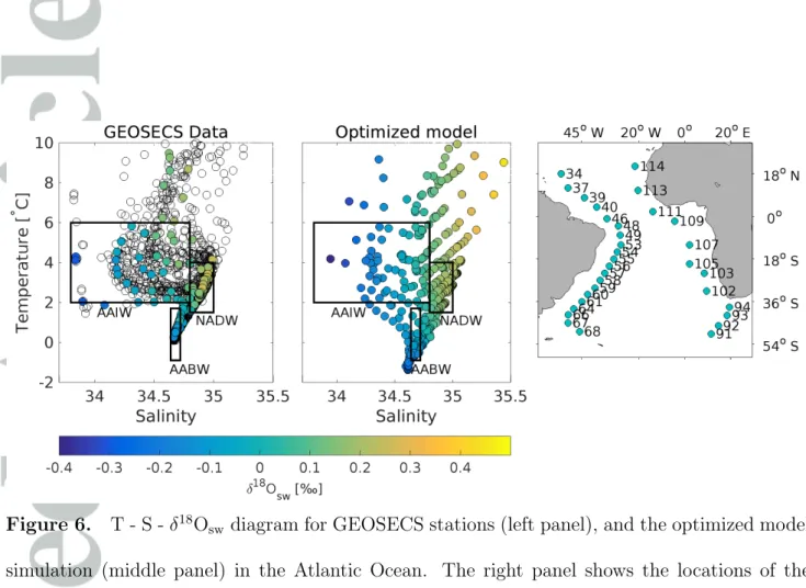
The optimized simulation is consistent with the δ¹⁸O_sw data in the deep ocean; the model-data misfit below a depth of approximately 500 m is smaller than the uncertainty of the data (Fig. 1). Figure 4 shows a vertical transect of δ¹⁸Osw through the Atlantic at 32.5^◦W from our data set (upper panel) and that of LeGrande and Schmidt [2006]

(lower panel). The water mass structure is clearly represented. In our data set the North Atlantic Deep Water (NADW) reaches about 4000 m depth and has a meanδ¹⁸O_sw value of 0.17‰, which is slightly too light compared with the observations (Table 5). The less enriched Antarctic Intermediate water (AAIW) overlies the NADW at a depth of about 1000 m (mean δ¹⁸O_sw of −0.07‰). The Antarctic Bottom Water (AABW) is the most isotopically depleted water mass with a mean value of−0.12‰.

Figure 5 shows depth profiles from our simulation, the data set ofLeGrande and Schmidt [2006] and observational data at four locations in the Atlantic Ocean. The first two are at GEOSECS stations [Ostlund et al., 1987] where¨ δ¹⁸O_sw data was available over most

of the water column. The third depth profile shows a set of unpublished δ¹⁸Osw data from the M57/2 METEOR cruise [Mulitza and Paul, 2003], which was not used for the optimization. The fourth depth profile shows data from one station of the WOCE A11 section [Meredith et al., 1999b]. Theδ¹⁸O_sw data from the GEOSECS and the WOCE A11 stations are included in the GISS data set and were therefore used in the optimization.

Both gridded data sets agree with the observational data at all four stations (root mean square error (RMSE) between 0.05‰ and 0.16‰). At GESOSECS station 29 our data set shows slightly too depleted values in the deep ocean, which corresponds to the slightly too light NADW (Table 5, RMSE of 0.11‰ compared to 0.08‰ for the data set of LeGrande and Schmidt [2006]). At GEOSECS station 56 the values of 0‰ at a depth of about 4000 m in our data set agree well with the observational data (RMSE of 0.07‰).

The data set ofLeGrande and Schmidt [2006] is slightly too enriched in this depth at this location (RMSE of 0.10‰). The depleted values in our simulation reflect the influence of the AABW, which extends approximately to the equator in our simulation (Fig. 4).

The influence of the AABW is also visible in the depth profile at the location of the unpublished data set close to the Namibian coast and in the data profile from the WOCE A11 section. Our simulation and that of LeGrande and Schmidt [2006] are consistent with the data at the M57/2 sites (RMSE of 0.08‰ for our simulation and 0.05‰ for the data set of LeGrande and Schmidt [2006]). Below a depth of 3000 m our simulation and the data set of LeGrande and Schmidt [2006] deviate, but no observational data is available for these depths. In the most southern profile the observational data show the influence of the more depleted AABW, which is well represented in our simulation (RMSE

of 0.09‰). The data set of LeGrande and Schmidt [2006] shows too enriched values in this area (RMSE of 0.16‰).

4. Discussion Surface Ocean

The optimized simulation agrees very well with the data as measured by the cost func- tion and by the additional metrics. It yields a substantial improvement from the first guess simulation (cost function reduction from 3.9 to 1.4 for δ¹⁸O_sw, Table 1). Our first-guess simulation had less enriched waters in the subtropical gyres and in the Mediterranean Sea than our optimized simulation and the observations (not shown). V¨olpel et al. [2017]

found similarly low enriched waters in their simulation and attributed this bias to the interaction of precipitation, evaporation, and the isotopic composition of evaporation.

The isotopic composition of evaporation directly depends on the isotopic composition of water vapor, which is prescribed as a boundary condition and a control variable in our optimization (Phase 2). After the optimization in Phase 1 the model agrees with salinity and temperature data, but the too lowδ¹⁸O_sw values remain in the subtropical gyres and in the Mediterranean Sea. During the optimization in Phase 2 the isotopic composition of water vapor was adjusted to slightly higher values in the subtropical areas, supporting the explanation of V¨olpel et al. [2017].

In the optimized simulation the isotopic composition of the surface waters in the Arctic Ocean still deviates from the data. Compared with our first guess simulation the optimized simulation is more depleted, but not depleted enough compared to observations. V¨olpel et al.[2017] found that their simulated surface waters in the Arctic Ocean are not depleted enough and attributed this to the fact that the highly depleted precipitation in the Arctic

does not have an influence on the isotopic composition of the seawater in areas with sea-ice.

The isotopic signal of precipitation is not preserved in the sea-ice model and is therefore not transported into the ocean when sea-ice is melting. As this study uses the same model code as V¨olpel et al. [2017], this deficiency is also apparent in our simulation. The low horizontal and vertical model resolution may lead to additional biases. The model does not include a land model and therefore does not explicitly simulate the isotopic composition of precipitation over river catchment areas. Instead the isotopic composition of river run- off is defined in the model by the isotopic composition of precipitation at the location of the river mouth. V¨olpel et al. [2017] analyzed the simulated isotopic composition of river run-off (their Figure 13) and its discharge amount. A model-data comparison showed a good agreement and they inferred that insufficient river discharge and the small errors in the simulated isotopic composition of river run-off have an insignificant influence on the simulation in coastal regions. The missing fractionation processes during sea-ice formation were also not thought to be important [V¨olpel et al., 2017]. The run-off and the first guess of the isotopic composition of precipitation used in this study are identical to those used inV¨olpel et al.[2017] . Our optimization leads to a negative adjustment (lowerδ¹⁸O_sw) of the isotopic composition of precipitation in the Arctic close to the Canadian coast between the Canadian Archipelago and the Bering Strait (not shown) resulting in locally slightly more depletedδ¹⁸O_sw values. The adjustment of the isotopic composition of precipitation directly affects the simulated δ¹⁸Osw through both precipitation and river run-off. The bias in the Arctic Ocean, however, is not completely balanced by the change ofδ¹⁸O_sw in precipitation close to the coast and no adjustments are found in the center of the Arctic.

We suppose that the reason for this is that the isotopic composition of precipitation does

not have an influence on the seawater in the center of the Arctic where sea-ice is present throughout the year. This supports the conclusion that the bias in the Arctic Ocean is not due to errors in the run-off and its isotopic composition, which is optimized in our simulation through precipitation at the coast, but mainly due to the missing isotopic surface flux in areas with sea-ice. This deficit cannot be improved by our control variables.

Simulations of other water isotope-enabled ocean-only and coupled atmosphere-ocean models deviate from the observational data typically in the enriched areas of the subtrop- ics, in the northern part of the Indian ocean, and/or in the isotopically depleted Arctic Ocean [e.g., Delaygue et al., 2000; Roche and Caley, 2013; Werner et al., 2016]. A com- paratively good agreement with the observational data is shown in the ocean-only model simulations by Xu et al. [2012], who prescribe the isotopic composition of precipitation and evaporation and used a salinity restoring, or by Paul et al. [1999], who prescribed a δ¹⁸Osw surface field as boundary condition.

If subgrid-scale variations of the data are taken into account in the model-data com- parison (Fig. 1, right panel), errors in the surface levels are especially high. We attribute this error to the stratification of Arctic surface waters that are not properly resolved by the coarse vertical resolution of the model. A comparison of the data set of LeGrande and Schmidt [2006] with the observations shows overall similar patterns but a smaller mismatch (Fig. 1) than our data set. Their data set has a finer horizontal and verti- cal resolution and the difference between Metric 1 and 2 (Fig. 1, left and right panel) is smaller for their data set indicating that small scale variations in the data are better represented in their data set. Highest errors in their data set are found in the Arctic

Ocean in areas with sea-ice. Their data set represents a yearly mean and they attribute the errors in the Arctic Ocean to the missing seasonal influence.

Deep Ocean

The water masses in the deep ocean are well represented in our data set (Fig. 4, 5, 6 and Table 5) and show a clear improvement compared to our first guess simulation and to the simulation ofV¨olpel et al. [2017] (their Table 3). In our first guess simulation the NADW was shallower, reaching until a depth of approximately 3300 m, and less enriched inδ¹⁸Osw

(mean value of 0.02‰). A too shallow simulation of the NADW is a common problem in coupled and ocean-only models [e.g. Weber et al., 2007; Yeager and Danabasoglu, 2012;

Jia, 2003]. The problem is thought to be caused by the incorrect simulation of density in areas of deep water formation. Constraining the simulation by temperature and salinity data leads to a more accurate representation of density and hence, after the optimization in Phase 1, the depth of the NADW cell appropriately reaches 4000 m. However, the mean δ¹⁸O_sw value in the NADW is still too low (0.01‰) after Phase 1. This likely reflects the missing influence of the enriched δ¹⁸O_sw from areas of deep water formation. After the optimization in Phase 2, the surface waters in the North Atlantic and the NADW are more enriched inδ¹⁸O_sw and agree better albeit not perfectly with the data (mean value of 0.17‰in the NADW compared with 0.21‰in the data). Figure 6 shows that the typical temperature and salinity values of the NADW are well represented in the model, which implies that the too lowδ¹⁸Osw values of the NADW in our simulation are not due to an inaccurate simulation of the water mass, but rather only due to an inaccurate simulation of its isotopic composition. The AABW, on the other hand, is slightly too cold and too fresh in the optimized simulation. The computed mean δ¹⁸O_sw value of −0.12‰ is too

high compared to −0.14‰ in the data. Figure 6, however, indicates that the isotopic composition is in fact accurate but the most depleted values were not included in the calculation of the mean value because the temperature and salinity ranges of the AABW in our simulation are slightly different to the typical values [Emery and Meincke, 1986].

The AAIW is also partly too cold compared to the typical values and has a too high mean δ¹⁸O_sw value (−0.07‰ compared to−0.09‰ in the data).

The too small δ¹⁸Osw values of the NADW might be related to the length of the opti- mization (400 years), which is not enough to fully transport the signal from the surface to the deep ocean [Wunsch and Heimbach, 2008]. Alternatively, a better result for the deep ocean might be obtained if spatially non-uniform observational uncertainty estimates are used in the cost function. Smaller errors for the deep ocean might result in a more accurate representation of the isotopic composition of the AAIW and the NADW or a more accurate simulation of the temperature and salinity ranges of the AABW and the AAIW.

To create their data set LeGrande and Schmidt [2006] used linear salinity-δ¹⁸O_sw rela- tionships based on observationalδ¹⁸O_sw data for distinct regions at the surface and water masses in the deep ocean. They additionally used a horizontal and vertical smoothing and subsequently, combined the data set with nearby observational δ¹⁸O_sw data for each depth level. Their data set agrees very well with the observational data (Fig. 1). In particular, their NADW ismore enriched than the NADW in our data set agreeing better with the observational data (Fig. 5, station 29). In areas with low data coverage, however, their technique results in sharp transitions at the borders of water masses, for example, at the border of the Southern Ocean (Fig. 4, lower panel), and between depth levels. As a

result the influence of the AABW is very small north of approximately 55^◦S (Fig. 4), and the deepest waters in that area are too enriched compared to the data (Fig. 5, WOCE A11 station). Even though the isotopic composition of the NADW is not as accurately represented in our data set as it is in the data set of LeGrande and Schmidt [2006], our data set provides clear improvements in other areas such as the South Atlantic Ocean.

The adjoint method provides the opportunity for interpolating sparse data in a physically meaningful way, that is, based on the model physics, and the resulting model simulation shows smooth transitions between water masses, for example, from the depleted waters of the Southern Ocean to the AAIW and AABW (Fig. 4, upper panel).

5. Conclusions

We presented the first physically consistent gridded data set of the seasonal δ¹⁸O_sw distribution of the global ocean. The data set is based on the dynamically consistent combination of observations and an ocean general circulation model with the adjoint method. It is obtained from a 400-year long optimized simulation of the model that is in agreement with a large number of monthly observational temperature, salinity and δ¹⁸Osw data. In terms of model-data misfit, the data set is similar to that of LeGrande and Schmidt [2006], but it brings major improvements in terms of the seasonal cycle and physical consistency. Our data set provides a smooth and physically meaningful inter- polation of the observational data and, especially in areas where the observational data coverage is low, it brings a large improvement in terms of smooth water mass transitions.

In the surface levels in the Arctic Ocean, however, the data set still deviates substan- tially from the observational data, mainly because the highly depleted isotopical signal of

Applying the method with a higher resolution model would likely provide better results, but also incur much higher computational costs. The isotopic composition of sea-ice, and especially the influence of the isotopic composition of precipitation falling onto the sea- ice, appear to be crucial for modeling Arctic surface δ¹⁸O_sw accurately. Including these explicitly in the model will likely lead to better results in the high latitudes.

We demonstrated high potential of the adjoint method for interpolating sparse data in a physically meaningful way and for substantially improving model simulations. The method makes it possible to create a data set that is based on the physical laws imple- mented in the model and that includes a seasonal cycle.

Our data set is publicly available and can serve in many applications where δ¹⁸O_sw data is required, for example to calibrate the relationship between δ¹⁸O_sw, δ¹⁸O_c and temperature, or to calibrate other paleoclimatological proxies. Especially in applications with proxy data with monthly resolution, for example from corals, the data set will be valuable.

Acknowledgments. C. Breitkreuz and T. Kurahashi-Nakamura are funded by the German Federal Ministry of Education and Research (BMBF) in the framework of the German Climate Modeling Initiative PalMod (www.palmod.de, FKZ: 01LP1511D and 01LP1505D). M. Losch is funded through AWI institutional funding, and M. Schulz and A. Paul through institutional funding of the University of Bremen.

We are grateful to Gavin Schmidt and co-authors for synthesizing the δ¹⁸Osw data and making them publicly available (https://data.giss.nasa.gov/o18data/), to Rike V¨olpel for providing the water isotope module for the MITgcm, and to two anonymous reviewers whose comments highly improved the quality and clarity of the manuscript.

The data set presented in this study (includingδ¹⁸Osw, potential temperature, and salin- ity) is freely available at PANGAEA (https://doi.pangaea.de/10.1594/PANGAEA.889922) on the original model (cubed-sphere) grid as well as interpolated to a regular 1^◦ grid. The MITgcm model code is freely available at http://mitgcm.org/public/source code.html.

References

Antonov, J. I., D. Seidov, T. P. Boyer, R. A. Locarnini, A. V. Mishonov, H. E. Garcia, O. K. Baranova, M. M. Zweng, and D. R. Johnson (2010), World Ocean Atlas 2009, Volume 2: Salinity, in Ed. NOAA Atlas NESDIS 69, edited by S. Levitus, pp. 1–184, U.S. Government Printing Office, Washington, D.C.

Cleroux, C., E. Cortijo, P. Anand, L. Labeyrie, F. Bassinot, N. Caillon, and J.-C. Duplessy (2008), Mg/Ca and Sr/Ca ratios in planktonic foraminifera: Proxies for upper water col- umn temperature reconstruction, Paleoceanography,23(3), doi:10.1029/2007PA001505.

Craig, H., and L. I. Gordon (1965), Deuterium and Oxygen 18 Variations in the Ocean and the Marine Atmosphere, Consiglio nazionale delle richerche, Laboratorio de geologia nucleare.

Dail, H. J. (2012), Atlantic Ocean Circulation at the Last Glacial Maximum: Inferences from Data and Models, Ph.D. thesis, Massachusetts Institute of Technology and the Woods Hole Oceanographic Institute, Massachusetts.

Delaygue, G., J. Jouzel, and J.-C. Dutay (2000), Oxygen 18-salinity relationship simulated by an oceanic general circulation model,Earth and Planetary Science Letters,178(1-2), 113–123, doi:10.1016/S0012-821X(00)00073-X.

Duplessy, J., L. Labeyrie, A. Juillet-Leclerc, F. Maitre, J. Duprat, and M. Sarnthein (1991), Surface salinity reconstruction of the North-Atlantic ocean during the last glacial maximum, Oceanologica Acta, 14(4), 311–324.

Emery, W., and J. Meincke (1986), Global water masses-summary and review,Oceanolog- ica acta,9(4), 383–391.

Emiliani, C. (1955), Pleistocene temperatures, The Journal of Geology, 63(6), 538–578, doi:10.1086/626295.

Errico, R. M. (1997), What is an adjoint model?, Bulletin of the American Meteorological Society,78(11), 2577–2591, doi:10.1175/1520-0477(1997)078¡2577:WIAAM¿2.0.CO;2.

Forget, G., J. Campin, P. Heimbach, C. Hill, R. Ponte, and C. Wunsch (2015), ECCO version 4: An integrated framework for non-linear inverse modeling and global ocean state estimation, Geoscientific Model Development, 8(10), 3071–3104, doi:10.5194/cp- 9-789-2013.

Ganachaud, A. (2003), Large-scale mass transports, water mass formation, and diffusivi- ties estimated from World Ocean Circulation Experiment (WOCE) hydrographic data, Journal of Geophysical Research: Oceans, 108(C7), doi:10.1029/2002JC001565.

Gat, J. R. (1996), Oxygen and hydrogen isotopes in the hydrologic cycle, Annual Review of Earth and Planetary Sciences, 24(1), 225–262, doi:10.1146/annurev.earth.24.1.225.

Gat, J. R., and R. Gonfiantini (1981), Stable isotope hydrology: Deuterium and Oxygen- 18 in the water cycle, Technical reports series no. 210, International Atomic Energy Agency, Vienna.

Gent, P. R., and J. C. Mcwilliams (1990), Isopycnal mixing in ocean circula- tion models, Journal of Physical Oceanography, 20(1), 150–155, doi:10.1175/1520-

0485(1990)020¡0150:IMIOCM¿2.0.CO;2.

Giering, R. (2000), Tangent linear and adjoint biogeochemical models, in Inverse meth- ods in global biogeochemical cycles, edited by P. Kasibhatla, M. Heimann, P. Rayner, N. Mahowald, R. Prinn, and D. E. Hartley, pp. 33–48, American Geophysical Union, Washington, DC.

Giering, R., and T. Kaminski (1998), Recipes for adjoint code construction,ACM Transac- tions on Mathematical Software (TOMS), 24(4), 437–474, doi:10.1145/293686.293695.

Gilbert, J. C., and C. Lemar´echal (1989), Some numerical experiments with variable- storage quasi-newton algorithms, Mathematical programming, 45(1-3), 407–435.

Gonfiantini, R. (1978), Standards for stable isotope measurements in natural compounds, Nature, 271(5645), 534, doi:10.1038/271534a0.

Griewank, A., and A. Walther (2008), Evaluating derivatives: principles and techniques of algorithmic differentiation, vol. 105, SIAM, Philadelphia.

Griffies, S. M., A. Biastoch, C. B¨oning, F. Bryan, G. Danabasoglu, E. P. Chas- signet, M. H. England, R. Gerdes, H. Haak, R. W. Hallberg, et al. (2009), Coordi- nated ocean-ice reference experiments (COREs), Ocean modelling, 26(1-2), 1–46, doi:

10.1016/j.ocemod.2008.08.007.

Groeneveld, J., and C. M. Chiessi (2011), Mg/Ca of Globorotalia inflata as a recorder of permanent thermocline temperatures in the South Atlantic, Paleoceanography, 26(2), doi:10.1029/2010PA001940.

Jacobs, S. S., R. G. Fairbanks, and Y. Horibe (1985), Origin and Evolution of Water Masses Near the Antarctic continental Margin: Evidence from H218O/H216O Ratios in Seawater, in Oceanology of the Antarctic Continental Shelf, edited by S. S. Jacobs,

pp. 59–85, American Geophysical Union, Washington, DC, doi:10.1029/AR043p0059.

Jia, Y. (2003), Ocean heat transport and its relationship to ocean circulation in the CMIP coupled models,Climate Dynamics, 20(2-3), 153–174, doi:10.1007/s00382-002-0261-9.

Khatiwala, S. P., R. G. Fairbanks, and R. W. Houghton (1999), Freshwater sources to the coastal ocean off northeastern North America: Evidence from H2 18O/H2 16O,Journal of Geophysical Research: Oceans, 104(C8), 18,241–18,255, doi:10.1029/1999JC900155.

K¨ohl, A., and D. Stammer (2008), Variability of the meridional overturning in the North Atlantic from the 50-year GECCO state estimation, Journal of Physical Oceanography, 38(9), 1913–1930, doi:10.1175/2008JPO3775.1.

K¨ohl, A., D. Stammer, and B. Cornuelle (2007), Interannual to decadal changes in the ECCO global synthesis, Journal of Physical Oceanography, 37(2), 313–337, doi:

10.1175/JPO3014.1.

Kurahashi-Nakamura, T., A. Paul, and M. Losch (2017), Dynamical reconstruction of the global ocean state during the Last Glacial Maximum,Paleoceanography,32(4), 326–350, doi:10.1002/2016PA003001.

Large, W. G., and S. G. Yeager (2004), Diurnal to decadal global forcing for ocean and sea- ice models: the data sets and flux climatologies,NCAR Technical Report TN-460+STR, CGD Division, National Center for Atmospheric Research Boulder, Colorado.

LeGrande, A. N., and G. A. Schmidt (2006), Global gridded data set of the oxy- gen isotopic composition in seawater, Geophysical Research Letters, 33(12), doi:

10.1029/2006GL026011.

Locarnini, R. A., A. V. Mishonov, J. I. Antonov, T. P. Boyer, H. E. Garcia, O. K.

Baranova, M. M. Zweng, and D. R. Johnson (2010), World Ocean Atlas 2009, Volume

1: Temperature, inEd. NOAA Atlas NESDIS 68, edited by S. Levitus, pp. 1–184, U.S.

Government Printing Office, Washington, D.C.

Losch, M., D. Menemenlis, J.-M. Campin, P. Heimbach, and C. Hill (2010), On the formulation of sea-ice models. Part 1: Effects of different solver implementations and parameterizations,Ocean Modelling,33(1), 129–144, doi:10.1016/j.ocemod.2009.12.008.

Lumpkin, R., K. G. Speer, and K. P. Koltermann (2008), Transport across 48^◦ N in the Atlantic Ocean, Journal of Physical Oceanography, 38(4), 733–752, doi:

10.1175/2007JPO3636.1.

Lund, D., J. Adkins, and R. Ferrari (2011), Abyssal Atlantic circulation during the Last Glacial Maximum: Constraining the ratio between transport and vertical mixing, Pa- leoceanography, 26(1), doi:10.1029/2010PA001938.

Macdonald, R., E. Carmack, F. McLaughlin, K. Falkner, and J. Swift (1999), Connections among ice, runoff and atmospheric forcing in the Beaufort Gyre,Geophysical Research Letters, 26(15), 2223–2226, doi:10.1029/1999GL900508.

Marshall, J., A. Adcroft, C. Hill, L. Perelman, and C. Heisey (1997), A finite-volume, incompressible Navier Stokes model for studies of the ocean on parallel computers, Journal of Geophysical Research: Oceans,102(C3), 5753–5766, doi:10.1029/96JC02775.

Mathien-Blard, E., and F. Bassinot (2009), Salinity bias on the foraminifera Mg/Ca ther- mometry: Correction procedure and implications for past ocean hydrographic recon- structions,Geochemistry, Geophysics, Geosystems,10(12), doi:10.1029/2008GC002353.

McCrea, J. M. (1950), On the isotopic chemistry of carbonates and a paleotemperature scale, The Journal of Chemical Physics, 18(6), 849–857, doi:10.1063/1.1747785.

Meredith, M. P., K. J. Heywood, R. D. Frew, and P. F. Dennis (1999a), Forma- tion and circulation of the water masses between the southern Indian Ocean and Antarctica: Results from δ¹⁸O, Journal of Marine Research, 57(3), 449–470, doi:

10.1357/002224099764805156.

Meredith, M. P., K. E. Grose, E. L. McDonagh, K. J. Heywood, R. D. Frew, and P. F.

Dennis (1999b), Distribution of oxygen isotopes in the water masses of drake passage and the south atlantic, Journal of Geophysical Research: Oceans, 104(C9), 20,949–

20,962, doi:10.1029/98JC02544.

MITgcm Group (2016), MITgcm User Manual,Online documentation, MIT/EAPS, Cam- bridge, MA 02139, USA.

Mulitza, S., and A. Paul (2003), Water Sampling for Stable Isotopes and Nutrient Analy- sis, inReport and preliminary results of METEOR Cruise M57/2, Walvis Bay - Walvis Bay, edited by M. Zabel and cruise participants, pp. 35–37, Berichte, Fachbereich Ge- owissenschaften, Universitt Bremen, Bremen, Germany.

Mulitza, S., D. Boltovskoy, B. Donner, H. Meggers, A. Paul, and G. Wefer (2003), Temperature: δ¹⁸o relationships of planktonic foraminifera collected from surface waters, Palaeogeography, Palaeoclimatology, Palaeoecology, 202(1), 143–152, doi:

10.1016/S0031-0182(03)00633-3.

Nocedal, J. (1980), Updating quasi-Newton matrices with limited storage, Mathematics of Computation,35(151), 773–782, doi:10.1090/S0025-5718-1980-0572855-7.

Ostlund, H. G., H. C. Craig, W. S. Broecker, D. W. Spencer, and GEOSECS¨ (1987), Shorebased measurements during the GEOSECS Atlantic expedition, doi:

10.1594/PANGAEA.824123.

Paul, A., S. Mulitza, J. P¨atzold, and T. Wolff (1999), Simulation of oxygen isotopes in a global ocean model, in Use of Proxies in Paleoceanography: Examples from the South Atlantic, edited by G. Fischer and G. Wefer, pp. 655–686, Springer, Berlin Heidelberg.

Roche, D., and T. Caley (2013), δ¹⁸O water isotope in the iLOVECLIM model (ver- sion 1.0)-Part 2: Evaluation of model results against observed δ¹⁸O in water samples , Geoscientific Model Development, 6(5), 1493–1504, doi:10.5194/gmd-6-1493-2013.

Ronchi, C., R. Iacono, and P. S. Paolucci (1996), The ”cubed sphere”: a new method for the solution of partial differential equations in spherical geometry, Journal of Compu- tational Physics,124(1), 93–114, doi:10.1006/jcph.1996.0047.

Schmidt, G., G. Bigg, and E. Rohling (1999), Global Seawater Oxygen-18 Database -v1.21, https://data.giss.nasa.gov/o18data/. Accessed 22 June 2016.

Tharammal, T., A. Paul, U. Merkel, and D. Noone (2013), Influence of Last Glacial Max- imum boundary conditions on the global water isotope distribution in an atmospheric general circulation model,Climate of the Past, 9(2), 789–809.

V¨olpel, R., P. Andr´e, A. Krandick, S. Mulitza, and M. Schulz (2017), Stable water isotopes in the MITgcm,Geoscientific Model Development,10(8), 3125–3144, doi:10.5194/gmd- 10-3125-2017.

Weber, S., S. Drijfhout, A. Abe-Ouchi, M. Crucifix, M. Eby, A. Ganopolski, S. Murakami, B. Otto-Bliesner, and W. Peltier (2007), The modern and glacial overturning circulation in the Atlantic ocean in PMIP coupled model simulations, Climate of the Past, 3(1), 51–64, doi:10.5194/cp-3-51-2007.

Werner, M., P. M. Langebroek, T. Carlsen, M. Herold, and G. Lohmann (2011), Stable wa- ter isotopes in the ECHAM5 general circulation model: Toward high-resolution isotope

modeling on a global scale, Journal of Geophysical Research: Atmospheres, 116(D15), doi:10.1029/2011JD015681.

Werner, M., B. Haese, X. Xu, X. Zhang, M. Butzin, and G. Lohmann (2016), Glacial–

interglacial changes in H₂¹⁸O, HDO and deuterium excess – results from the fully cou- pled ECHAM5/MPI-OM Earth system model, Geoscientific Model Development, 9(2), 647–670, doi:10.5194/gmd-9-647-2016.

Wunsch, C. (1996), The ocean circulation inverse problem, Cambridge University Press.

Wunsch, C., and P. Heimbach (2008), How long to oceanic tracer and proxy equilibrium?, Quaternary Science Reviews,27(7-8), 637–651, doi:10.1016/j.quascirev.2008.01.006.

Xu, X., M. Werner, M. Butzin, and G. Lohmann (2012), Water isotope variations in the global ocean model MPI-OM,Geoscientific Model Development,5(3), 809–818, doi:

10.5194/gmd-5-809-2012.

Yeager, S., and G. Danabasoglu (2012), Sensitivity of Atlantic meridional overturning circulation variability to parameterized Nordic Sea overflows in CCSM4, Journal of Climate, 25(6), 2077–2103, doi:10.1175/JCLI-D-11-00149.1.

Table 1. Overview over the reduction of the cost function and lengths of the cost function intervals during the carry-over optimization process. The termsJ_misfit⁰ andJ_ctrl⁰ are the normalized values, that is, the model-data misfit (J_misfit) and the deviation from the first guess control variables (Jctrl) divided by the respective number of model-data comparisons/control variables.

Note that for the optimization the original termsJ_misfit and J_ctrl were used. For J_misfit respective values for temperature, salinity andδ¹⁸O_sw are given. According to the theory of aχ²-test a value of one indicates agreement of the model with the observations within their respective uncertainties or an adjustment of the control variables within the assumed uncertainties. Note that J_ctrl⁰ is zero at the beginning of the optimization as the control variables were not yet modified.

J_misfit⁰

Run length Cost function interval Temperature Salinity δ₁₈O J_ctrl⁰

1st guess spin-up 100 years 3.4 6.1 3.9 0

(4000 years) Phase 1

20 years 15 years 0.9 1.1 - 1.4·10⁻¹

35 years 30 years 0.9 1.0 - 1.7·10⁻¹

55 years 40 years 0.9 1.2 - 1.8·10⁻¹

80 years 50 years 1.0 1.5 - 1.8·10⁻¹

200 years 150 years 1.0 1.3 - 2.0·10⁻¹

400 years 100 years 1.1 1.7 - 2.0·10⁻¹

Spin-up after Phase 1 100 years 1.5 2.2 4.4

(4000 years) Phase 2

100 years 10 years - - 1.5 4.7·10⁻⁴

200 years 10 years - - 1.5 4.8·10⁻⁴

400 years 100 years (1.1) (1.7) 1.4 4.8·10⁻⁴

Table 2. Control variables with assumed prior uncertainties (one standard deviation, σ) used in the optimization and normalized cost for the deviations from the first guess of the respective control variable at the end of the optimization (J_ctrl⁰ ).

Symbol Control variable Unit σ J_ctrl⁰

T0 Initial temperature ^◦C 3.16·10⁰ 5.0·10⁻¹ S₀ Initial salinity - 3.16·10⁻¹ 3.7·10⁻¹ Φ_0,1 Initial tracer Φ₁ = H¹⁶₂ O mol·m⁻³ 3.16·10² 1.8·10⁻³ Φ_0,2 Initial tracer Φ₂ = H¹⁸₂ O mol·m⁻³ 1.00·10¹ 2.5·10⁻⁵ F₁ Surface (2-m) air temperature K 3.16·10⁰ 5.3·10⁻² F2 Surface (2-m) specific humidity kg·kg⁻¹ 3.16·10⁻³ 1.4·10⁻¹ F₃ Precipitation m·s⁻¹ 3.16·10⁻⁸ 2.7·10⁻¹ F₄ Surf. (10-m) zonal wind vel. m·s⁻¹ 3.16·10⁰ 2.1·10⁻¹ F₅ Surf. (10-m) meridional wind vel. m·s⁻¹ 3.16·10⁰ 2.6·10⁻¹ F₆ Downward shortwave radiation W·m⁻² 1.00·10¹ 2.9·10⁻³ F7 Downward longwave radiation W·m⁻² 1.00·10¹ 3.3·10⁻³ F₈ Isotopic ratio of precipitation - 1.00·10⁻³ 1.1·10⁻⁵ F₉ Isotopic ratio of water vapor - 1.00·10⁻³ 1.7·10⁻⁵ K Vertical diffusion coefficient m²·s⁻¹ 1.00·10⁻⁵ 8.1·10⁻²

Table 3. Weights (w) used in the cost function term J_eq (Phase 1 of the optimization).

Symbol Variable w

T yearly mean temperature 10⁸

η yearly mean sea surface elevation 10⁸ AMOC yearly mean strength of southward transport 10⁴

at 45^◦N in the Atlantic Ocean

Table 4. Imposed minimum and maximum values for the control variables. The values were chosen either by the model developers or by the authors (isotopic ratios) for physical meaning- fulness (minimum values for precipitation, specific humidity and downward shortwave radiation) or plausibility.

Variable Unit Minimum Maximum

Precipitation m·s⁻¹ 0 2.0·10⁻⁶

Specific humidity kg·kg⁻¹ 0 1.0·10⁻¹ Downward shortwave radiation W·m⁻² 0 600

Air temperature K 183 343

Isotopic ratio in precipitation - 1.92·10⁻³ 2.02·10⁻³ Isotopic ratio in water vapor - 2.13·10⁻³ 2.215·10⁻³

Table 5. δ¹⁸O_sw characteristics of the main water masses in the the Atlantic (AAIW - Antarctic Intermediate Water, NADW - North Atlantic Deep Water, AABW - Antarctic Bottom Water) in our optimized simulation and in the GEOSECS data. The water masses are defined according to the temperature and salinity limits of Emery and Meincke [1986].

AAIW NADW AABW

Optimized simulation

δ¹⁸O_sw range (‰) −0.47 - 0.13 0.05 - 0.30 −0.20 - −0.01

δ¹⁸O_sw mean (‰) −0.07 0.17 −0.12

δ¹⁸O_sw standard deviation (‰) 0.10 0.04 0.04 Observational data [V¨olpel et al., 2017]

δ¹⁸O_sw range (‰) −2.50 - 1.41 −0.49 - 0.88 −0.31 - 0.00

δ¹⁸O_sw mean (‰) −0.09 0.21 −0.14

δ¹⁸O_sw standard deviation (‰) 0.42 0.09 0.08