Concentration and Size Distribution of Microparticles in the NGRIP Ice Core (Central Greenland) during the Last Glacial Period

of Microparticles in the

NGRIP Ice Core (Central Greenland) during the Last Glacial Period

Dissertation zur Erlangung des

Doktorgrades der Naturwissenschaften

im Fachbereich Geowissenschaften der Universit¨at Bremen

vorgelegt von

Urs Ruth

Bremen, im April 2002

Universit¨at Heidelberg f¨ur Polar- und Meeresforschung Im Neuenheimer Feld 229 Columbusstraße

D-69120 Heidleberg D-27568 Bremerhaven Urs.Ruth@iup.uni-heidelberg.de

This is a reprint of a dissertation submitted to the

Department of Geosciences of the University of Bremen in April 2002.

It is published as report number 428 of the Berichte zur Polar- und Meeresforschung (ISSN 1618-3193). It is available electronically at:

http://www.ub.uni-heidelberg.de/archiv/2291

Die vorliegende Arbeit ist die inhaltlich unver¨anderte Fassung einer Dissertation, die im April 2002 dem Fachbereich Geowissenschaften der Universit¨at Bremen vorgelegt wurde.

Sie ist in den Berichten zur Polar- und Meeresforschung (ISSN 1618-3193) als Band Nummer 428 ver¨offentlicht Die Arbeit ist elektronisch erh¨altlich unter:

http://www.ub.uni-heidelberg.de/archiv/2291

Abstract 1

Kurzzusammenfassung 2

1 Introduction 3

2 The mineral aerosol 7

2.1 Origin and composition . . . 7

2.2 Entrainment . . . 8

2.3 Transport . . . 10

2.4 Deposition . . . 11

2.5 Size distribution . . . 13

3 Particle counting and sizing 16 3.1 Measuring techniques for microparticle analysis . . . 16

3.2 The laser sensor: measurement principle and operational parameters . . 17

3.3 The laser sensor: size calibration . . . 19

3.4 Determination of flow rates . . . 21

3.5 Parameterization of the size spectrum . . . 22 4 High resolution microparticle profiles at NGRIP: Case studies of the

calcium – dust relationship 28

5 Continuous record of microparticle concentration and size distribu- tion in the central Greenland NGRIP ice core during the last glacial

period 44

6 Nitrate in Greenland and Antarctic ice cores: a detailed description

of post-depositional processes 77

i

7 Summary and Outlook 98 A Size calibration of the laser sensor – details and listings 101

B Die Schmelzapparatur 105

B.1 Vorteile des kontrollierten L¨angsschmelzens . . . 105

B.2 Anforderungen an die Schmelzanlage . . . 106

B.3 Beschreibung der Apparatur . . . 107

B.3.1 K¨uhlsystem mit Probenaufnahme und Schmelzkopf . . . 107

B.3.2 Schlauchsystem mit Pumpen . . . 110

B.3.3 Nachweissysteme . . . 112

B.3.4 Probenabf¨ullung . . . 113

B.3.5 Datenaufnahme und Prozesssteuerung . . . 114

B.4 Kalibration, Blanks und Tiefenaufl¨osung . . . 115

B.5 Vorbereitung der Proben im K¨uhllabor . . . 117

B.6 Datenauswertung . . . 118

C Die elektrolytische Leitf¨ahigkeit 120 C.1 Physikalische Grundlagen . . . 120

C.2 Durchflussmesszellen f¨ur den CFA- oder FIA-Betrieb . . . 122

C.3 Reduzierte Leitf¨ahigkeit . . . 122

D Die Azidit¨at 124 D.1 pH-Wert und Azidit¨at . . . 124

D.1.1 Der pH-Wert . . . 124

D.1.2 Das Carbonat-System . . . 124

D.1.3 Die Azidit¨at . . . 126

D.2 Messung der Azidit¨at . . . 127

D.2.1 Grundlagen . . . 127

D.2.2 Messaufbau . . . 128

D.2.3 Kalibration . . . 130

Bibliography 133

Danksagung 145

Abbreviations 147

in the deep North Greenland Ice Core Project (NGRIP) ice core continuously from 1405 m to 2930 m depth. The measurements were accomplished using a novel, optical detector which is based on laser light attenuation by individual particles. The device works on a flow-through basis, and together with sample preparation via continuous melting it allows for very time efficient analyses at high depth resolution. The presented work also covers the partial development and the application of a continuous ice core melting setup as well as analytical systems of electrolytical conductivity and acidity.

In the NGRIP ice core, the concentration of microparticles was found to be around 70 µg kg⁻¹ during Preboreal Holocene and 8000 µg kg⁻¹ during the last glacial max- imum (LGM). Variations by typically a factor of 8 of the insoluble particle mass and number concentrations were encountered across the rapid Dansgaard/Oeschger transi- tions within the last glacial period.

The (Ca²⁺)/(insoluble microparticle) mass ratio was investigated in various selected core sections. Relatively low Ca²⁺ contents were found concurring with high crustal concentrations. Such systematic variations were observed on long time scales (>1000 years) and also on seasonal to multi-annual time scales. Strong enhancements of the (Ca²⁺)/(insoluble microparticle) ratio by up to a factor of 3 were found during volcanic events due to increased dissolution of CaCO₃ by volcanogenic acids. These findings limit the use of Ca²⁺ as an unequivocal quantitative reference species for mineral dust.

Systematic variations of the size distribution were observed with the tendency to- wards larger particles during colder climates. The lognormal mode of the volume distribution was found at about 1.3 µm diameter during Preboreal Holocene and 1.7 µm diameter during peak LGM. Size changes occurred largely synchronous with con- centration changes. By use of a simple, semi-quantitative model picture it is inferred that (i) the observed variations mainly reflect changes of the airborne particle size dis- tribution over Greenland, and that (ii) these size changes probably are a consequence of changed particle transit times from the source to the ice sheet. Long range trans- port times shorter by 25% during the LGM with respect to Preboreal Holocene can explain the observed size changes. Further, it is estimated that these changes in trans- port can account for a concentration increase of less than 1 order of magnitude and clearly cannot explain the total observed concentration increase during LGM. There- fore, source intensifications must have occurred synchronously to changes of long range transport. Furthermore, a higher variability of the lognormal mode was observed dur- ing warmer climates as reflected by increased point-to-point variability and also by increased distribution widths for the multi-year samples considered. It thus is inferred that atmospheric circulation was more variable during such times.

1

tiefen Eisbohrkern des North Greenland Ice Core Project (NGRIP) kontinuierlich von 1405 m bis 2930 m Tiefe untersucht. Die Messungen wurden mit einem neuartigen, optischen Detektor durchgef¨uhrt, dessen Nachweisverfahren auf der Abschw¨achung von Laserlicht durch einzelne Partikel beruht. Das Ger¨at arbeitet im kontinuierlichen Durchfluss, und in Verbindung mit einer kontinuierlichen Schmelzapparatur erm¨oglicht es sehr Zeit-effiziente Analysen bei gleichzeitig hoher Tiefenaufl¨osung. Die vorliegende Arbeit umfasst außerdem die teilweise Entwicklung sowie die Anwendung von einer kontinuierlichen Eiskern-Schmelzapparatur und von Analysesystemen f¨ur elektrolyti- sche Gesamtleitf¨ahigkeit und Azidit¨at.

Im NGRIP Eiskern betrug die Mikropartikelkonzentration ca. 70µg kg⁻¹ w¨ahrend des pr¨aborealen Holoz¨ans und ca. 8000 µg kg⁻¹ w¨ahrend des letzten glazialen Maxi- mums (LGM). Starke Variationen der Massen- und Anzahlkonzentration um typisch einen Faktor 8 wurden w¨ahrend der eiszeitlichen Dansgaard/Oeschger-Ereignisse fest- gestellt.

Das Massenverh¨altnis (Ca²⁺)/(unl¨osliche Partikel) wurde in mehreren Tiefenhori- zonten untersucht. Relativ niedrige Ca²⁺-Gehalte wurden w¨ahrend hoher Staubkonzen- trationen beobachtet. Solche systematischen Variationen wurden sowohl auf langen Zeitskalen (> 1000 Jahre) als auch auf saisonalen bis multiannualen Zeitskalen fest- gestellt. Erh¨ohungen des (Ca²⁺)/(unl¨osliche Partikel)-Verh¨altnisses um mehr als einen Faktor 3 wurden in Vulkanhorizonten beobachtet und sind vermutliche auf verst¨arkte Aufl¨osung von CaCO₃ durch vulkanogene S¨aure zur¨uckzuf¨uhren. Dies schr¨ankt die Verwendung von Ca²⁺ als eindeutige, quantitative Referenz f¨ur Mineralstaub ein.

Es wurden systematische Variationen der Gr¨oßenverteilung beobachtet mit einem Trend zu gr¨oßeren Partikeln in k¨alteren Klimaperioden. Die log-normale Mode der Volumenverteilung liegt im pr¨aborealen Holoz¨an bei ca. 1.3 µm Durchmesser und bei ca. 1.7 µm Durchmesser im Hoch-LGM. Ver¨anderungen von Gr¨oße und Konzentra- tion treten weitgehend gleichzeitig auf. Mit Hilfe eines einfachen, halb-quantitativen Modellbildes kann geschlossen werden, dass (i) die beobachteten Gr¨oßenvariationen haupts¨achlich Ver¨anderungen der luftseitigen Gr¨oßenverteilung ¨uber Gr¨onland wider- spiegeln und dass (ii) diese Gr¨oßenver¨anderungen vermutlich auf Ver¨anderungen der Transportzeit der Partikel von der Quelle zum Eisschild zur¨uck gef¨uhrt werden k¨onnen.

Hierbei k¨onnen um 25% k¨urzere Ferntransportzeiten w¨ahrend des LGMs die beobachtete Gr¨oßenver¨anderung erkl¨aren. Desweiteren kann abgesch¨atzt werden, dass solche k¨urze- ren Transportzeiten eine Konzentrationserh¨ohung von weniger als einer Gr¨oßenordnung bewirken und nicht die beobachtete Konzentrationserh¨ohung w¨ahrend des LGMs erkl¨a- ren k¨onnen. Daher m¨ussen gleichzeitig zu Ver¨anderungen des Ferntransportes auch Ver¨anderungen der Quellst¨arke eingetreten sein. Außerdem wurde eine h¨ohere Vari- abilit¨at der log-normalen Mode w¨ahrend warmer Klimaperioden beobachtet; daraus kann geschlossen werden, dass die atmosph¨arische Zirkulation zu solchen Zeiten vari- abler gewesen ist.

2

Introduction

Ice cores provide a wealth of paleo-climatic information. Well-stratified ice core records can reach back in time continuously for several 100 000 years. The spectrum of archived information is immense and reaches from stable isotope ratios of the water molecule, which allow a temperature reconstruction of the atmosphere, over past atmospheric aerosol content to greenhouse gas concentrations. This makes it possible to study past climates and the degree of natural climate variability.

The ice core record from Camp Century (North West Greenland) for example re- vealed large climatic fluctuations that occurred during the last glacial period with extremely rapid transitions between cold and warm states [Dansgaard et al., 1969].

And the record from Vostok (East Antarctica) showed amongst other things that the present atmospheric concentration of the greenhouse gas CO₂ is unprecedented during the last 420 000 years and that also the current rate of increase exceeds that of previous, naturally occurring changes [Petit et al., 1999].

Ice core research not only provides reconstructions of past environmental conditions.

It also allows to study the causes and feed back mechanisms of past climate changes because multiple atmospheric trace species are stored in one archive simultaneously.

The insights from ice core studies have a lot of implications for climate research and ultimately yield crucial information also for the understanding of today’s climate. Such knowledge is essential for reliable assessments of anthropogenic climate change for the past as well as for the future.

The reconstruction of past atmospheric aerosol loads is a central topic in ice core research. Aerosols are solid or liquid particles suspended in the atmosphere. They have a driving influence on Earth’s climate through multiple mechanisms (e.g. [Prospero et al., 1983; Ramanathan et al., 2001]). They enhance the scattering and absorption of solar radiation (direct climatic forcing), but they also produce brighter clouds that

3

reduce the amount of solar irradiance reaching the ground (indirect climatic forcing).

This is also the case for the mineral dust aerosol (e.g. [Sokolik et al., 2001]). Mineral dust deposited in Greenland consists of windblown microparticles that are entrained into the atmosphere during dust storms and are carried long distances. The main source of mineral dust transported to Greenland has been traced to the East Asian deserts [Biscaye et al., 1997].

The concentration of dust in Greenlandic ice cores was found 100-fold increased during the Last Glacial Maximum (LGM, about 20 000 years ago) compared to present day (e.g. [Steffensen, 1997]), which involved strong alterations of paleoclimatic forcings.

Yet, the mineral dust concentrations are not only a climatic forcing factor, they also are indicative for past climatic situations. However, the reasons for the strong increase observed are still disputed. In particular it is uncertain to which extend it was caused by enhanced source strength (which would imply an increased atmospheric dust load along the whole transport pathway) or to which extent it resulted from more efficient transport of dust to Greenland (which would imply an increased dust load at high latitudes especially but less so at lower latitudes).

Mineral dust holds a soluble and an insoluble fraction, the latter of which also is called ’(insoluble) microparticles’. Calcium (Ca) is the most abundant element of the soluble fraction; and since Ca²⁺ can be readily measured using standard ion chro- matography (IC) the Ca²⁺ion concentration has often been taken as a proxy parameter for dust so far. However, the ratio of Ca²⁺ to insoluble dust is known to be variable [Steffensen, 1997], and systematic investigations of this variability are needed. Such investigations have not been performed yet as not much data of the total, i.e. the solu- ble and insoluble dust mass have been available. This is because the Coulter counting technique, which is the standard measurement technique for insoluble microparticles, is very work intensive as well as susceptible to perturbations.

Dust permits not only the study of its concentration or composition but also of its size distribution. The size distribution is expected to be modified by the transport and deposition of particles. Therefore, archives of aeolian dust may allow far-reaching inferences on the properties of past atmospheric transport. However, until now the interpretation of observed changes of the size distribution has been poor and also not much data has been available.

The drilling of the North Greenland Ice Core Project (NGRIP) ice core enabled further investigations of the mineral dust aerosol in polar ice. The NGRIP drill site is located in central Greenland at (75.1N,42.3W) about 300 km NNW of the summit region on an ice divide. Figure 1.1 shows the location of the NGRIP core and other Greenlandic ice coring sites.

Camp Century

1963 - 1966 1390 m

Dye3

1979 - 1981 2037 m

Summit

GRIP / GISP 2

1990 - 1992 3029 m

North-GRIP

1998 - ongoing 3001 m by year 2001 (3085 m expected)

0 400 km

Figure 1.1: Map of Greenland showing the location of deep ice coring sites. Periods of active drilling and ice thicknesses are indicated. Modified after [Fischer, 1997].

During the NGRIP-2000 field season an analytical laboratory was operated and extensive analyses of tracer concentrations were performed. These included the deploy- ment of a novel type of microparticle counter which is based on laser light attenuation.

The new counter is easy handling and in combination with a continuous ice core melt- ing setup allows for very efficient sample processing already in the field. This effort resulted in a high resolution profile of microparticle concentration and size distribution covering almost the entire last glacial period.

In this work, the novel particle detector is described, and a method of size calibra- tion is presented (chapters 3, 4, 5, and appendix A). In case studies the Ca²⁺/(insoluble dust) mass ratio is investigated for long term as well as short term variations (chapter 4). In chapter 5 the microparticle concentration and size distribution profiles from the NGRIP core are presented and discussed. A highly simplified but quantitative model picture is developed for the interpretation of the particle size.

Chapter 6 is not directly connected to the NGRIP particle measurements. It deals with the conservation of atmospheric HNO₃ in ice cores and with post-depositional changes of the NO₃ concentration in polar ice.

The work of chapters 4 and 6 is in press at Annals of Glaciology, Vol. 35; the work presented in chapter 5 is submitted to the Journal of Geophysical Research for publication.

Additional activities In the course of this work extensive effort was put into the continuing development and operation of a continuous ice core melting setup for home laboratory applications. This not only included the analysis of microparticles, which is described methodically in chapter 3, but also the dedicated deployment of the elec- trolytical conductivity signal. Furthermore, a setup for the direct measurement of acidity was established. These developments were applied for comprehensive analyses of the 180 m long B25 ice core from Berkner Island (Antarctica) and several shal- low firn cores from the new drilling cite in Severnaya Semlya (Russian Arctic). The Berkner Island core, which spans about the last 1200 years, was analyzed in a con- tinuous flow type fashion for electrolytical conductivity, microparticle content, and Ca²⁺- and NH⁺₄-concentrations in subseasonal resolution. About 2000 discrete samples were automatically prepared and as yet have partly been measured for F⁻, MSA⁻, Cl⁻, NO⁻₃, SO²⁻₄ and H⁺ concentrations. This will be the basis for a core chronology through annual layer counting and is expected to reveal the history of the Weddell Sea region. The scientific results of these measurements will be presented elsewhere, however, selected methodical aspects are documented here in appendices B – D (in German).

The mineral aerosol

2.1 Origin and composition

The mineral aerosol consists of mineral material suspended in the atmosphere. It may be present as fine grained particles or in a dissolved form within water droplets or ice crystals. In ice core analyses, a distinction between the soluble fraction and the insoluble one is useful, the latter of which is also referred to as mineral microparticles.

Commonly, the mineral aerosol is also called mineraldust. It originates predominantly from large deserts or semiarid areas that are subject to wind erosion.

In the source areas loose, fine grained material is produced by weathering pro- cesses. Pye [1987] distinguishes between frost weathering, aeolian abrasion, insolation weathering, salt weathering, chemical weathering, and others. All theses mechanisms are not mutually exclusive but may occur in combinations with each other. Physi- cal weathering causes the breakage of crystalline material due to increased mechanical stress. Chemical weathering causes the disintegration of parent material by dissolu- tion along lines of crystal weakness through chemical reactions. Often CO₂ or organic acids present in the soil enhance this process. Physical weathering mechanisms tend to prevail in cold and arid climates, whereas chemical weathering is favored by warm and wet climates. The different types of weathering are therefore associated with different mineralogical compositions (e.g. kaolinite vs. chlorite).

The largest soluble fraction of aeolian dust is made up by Calcium carbonate CaCO₃. Therefore Ca²⁺ ions are often taken as a proxy parameter for dust in ice cores.

However, the elemental and mineralogical composition of dust underlies regional vari- ations which also affects its Ca content. The Ca content of loesses, for example, ranges from below 10% to more than 30% [Pye, 1987]. The Aluminum content of crustal material is more homogeneous (about 8% for average continental crust [Bowen, 1979]).

7

Therefore, Al surely would be a better proxy for the concentration of the insoluble dust fraction, and probably also for the total dust concentration. But as oppose to Ca, Al cannot be measured easily by standard IC.

Archives of aeolian dust hold information on climatic situations in the source areas and about past wind fields. Terrestrial sediment profiles (e.g. [Sarnthein, 1978; Lamy et al., 1999; Lagroix and Banerjee, 2002]), marine sediment cores (e.g. [Janecek and Rea, 1985; Rea, 1994]), and ice cores (e.g. [Thompson and Mosley-Thompson, 1981;

Steffensen, 1997; Petit et al., 1999]) have been studied as archives of aeolian dust.

From these it has been inferred that during the last glacial period the atmospheric dust load was much higher and that wind or storm patterns may have been different.

Provenance studies of aeolian dust can be based on particle mineralogy and isotopic composition. The mineralogy depends on the parent material and on environmental conditions in the source areas (e.g. [Maggi, 1997]). The isotopic composition of mineral materials differs in rocks from different lithologies and geologic ages, which hold indi- vidual isotope ratios e.g. of ²⁰⁶Pb /²⁰⁷Pb or ⁸⁷Sr /⁸⁶Sr. As these ratios are preserved during weathering and transport they may be deployed to identify the source region of windblown microparticles. This was done by Biscaye et al. [1997] and Grousset et al. [1992] who thereby identify East Asian deserts respectively Patagonian deserts as the most probable source areas for dust carried to Greenland and Antarctica. For Greenland it seems surprising that neither the Sahara nor the North American deserts are the dominant sources. For dust transport during the Pleistocene, the role of East Siberia remains unclear to date. This region probably was ice free polar desert during the last glacial period [Felzer, 2001], however, no reference samples for isotopic com- parisons have yet been available to confirm or negate its importance as a dust source to Greenland during the last glacial.

2.2 Entrainment

Wind erosion may take place on soils that are unprotected by vegetation and sufficiently dry. During a dust storm particles are moved horizontally, and three distinct modes of transport have been identified: surface creep, saltation and suspension [Bagnold, 1941]. Large soil particles (typically greater than 0.5 mm) move in a rolling fashion called surface creep, whereas smaller particles (typically 0.05 to 0.5 mm) move in a hopping manner called saltation. Fine particles (typically smaller than 0.05 mm) may remain in suspension for longer periods of time. About 50% to 80% of the total soil movement takes place through saltation, whereas only ≈ 1% of the total mass is

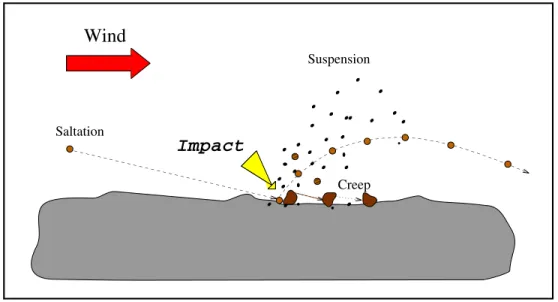
Figure 2.1: Schematic illustration of particle entrainment by saltation bombardment.

Modified after [Hua, 1999].

moved by suspension [Gillette et al., 1974]. Although suspension makes up only a small fraction of the total soil movement it is the only process that allows particles to get associated with long range transport and be carried long distances. These particles are usually referred to as dust particles, whereas the others are called sand particles.

Most notable is that saltating grains are a driving mechanism for all three modes of particle movement. This is illustrated in Figure 2.1. The saltating grains are usually lifted a few 10 cm above the ground and as they impact on the surface part of their kinetic energy is transferred to other particles. This may trigger surface creep and lift other small and fine particles into the air resulting in a chain reaction. This process is called saltation bombardment. It may also cause the disintegration of polycrystalline particles and thus the production of fine grained material.

The mobilization of dust underlies various environmental influences. First of all (and trivial) is the occurrence of strong surface winds or storms, and second the surface wind speed u during such events. In field experiments the flux of fine particles was found to depend onu^j with the exponentj ranging from 2 [Alfaro and Gomes, 2001] to 4 [Gillette and Passi, 1988]. The efficiency of saltation bombardment crucially depends on soil moisture content, i.e. on the aridity of the source region. Further, the presence of non-erodible objects such as vegetation or rocks may be rate limiting, as they decrease the surface wind speed and act as catchers of particles yet aloft. The soil texture also plays an important role for dust production, as surface crusts lessen the amount of material available for mobilization. The entrainment of dust in general is a strongly

Figure 2.2: Schematic of a dust storm of the squall-line type; from [Pye, 1987].

episodic process with a few single events contributing almost the total annual flux.

2.3 Transport

Once lifted off the ground the small suspended microparticles may be lifted further to long range transport heights and carried long distances. During transport they are exposed to removal processes by wet and dry deposition. Wet deposition is all removal related to precipitation including in-cloud (”rain-out”) and below-cloud (”wash-out”) scavenging as well as nucleation scavenging, whereas dry removal includes e.g. sedi- mentation or impaction. Uplift may be very efficient in convective cells as sketched in Figure 2.2 but wet removal may also be very strong there. The tropics with the inner tropical convergence zone and with high rates of precipitation resemble an effective barrier against dust transport across the equator. This results in separate dust cycles in the northern and southern hemispheres.

Long range transport takes place above the planetary boundary layer. The dust is transported in dust plumes or hazes. For dust delivered to Greenland zonal transport from the East Asian source areas is achieved in the regions of the planetary westerly winds. Meridional transport into the polar cell is provided by the low pressure systems that develop along the polar front. During the last glacial period the temperature gradient between the Arctic and the tropics presumably was much stronger than today

due to a larger temperature difference between the polar regions and the tropics as well as due to an equatorward extended polar vortex. This resulted in increased baro- clinicity and may have strengthened both the zonal as well as the meridional transport [Andersen and Ditlevsen, 1998;Tegen and Rind, 2000].

Dust transport to Greenland is influenced by the seasonal monsoon cycle in the source region and by the seasonal weakening and strengthening of the polar front around the Arctic. This leads to seasonally occurring so-called Arctic Haze-bands [Rahn and Borys, 1977] and also results in a strong seasonality of the dust flux to the Greenlandic ice sheet. This is mirrored by a pronounced maximum of the microparticle concentration in snow observed in late winter / early spring [Steffensen, 1985].

During transport significant in-cloud processing may occur. A large percentage of clouds evaporates again without producing rain. This may lead to a series of washing and coating for a particle. In cloud droplets the soluble fraction may be removed from the particle, and during subsequent evaporation of the droplet all dissolved material present may turn into a coating around the particle. Hereby the original composition of the particle is not necessarily restored as fractionating processes may occur or ad- ditional dissolved matter may have been present in the droplet. In-cloud processing is capable of changing the composition as well as the size distribution of airborne particles [Wurzler et al., 2000].

Often archives of aeolian dust are interpreted in the context of atmospheric circula- tion. AsRea[1994] already pointed out it should be noted that dust storms occur most episodically. Therefore the information drawn from the dust deposits is characteristic for storm events predominately and not necessarily also for mean atmospheric flow.

2.4 Deposition

Aerosols are moved from the air to the ground by numerous processes, and a classifi- cation into wet and dry deposition is useful. Wet deposition is associated with precip- itation events whereas dry deposition includes all processes not directly connected to precipitation.

Particles are incorporated into precipitation via several mechanisms: They are con- sumed as condensation nuclei during the formation of clouds. Further, Brownian dif- fusion especially causes small particles to move into already existing cloud droplets. In addition a ”micro advection” of particles is caused by Stefan-flow, which is a stream of air and water vapor towards a condensing cloud droplet.

Apart from these in-cloud processes there is the below-cloud scavenging (or ”wash-

Figure 2.3: Illustration of dry deposition mechanisms for particles to snow; from [David- son et al., 1996].

out”) of particles. Here, particles are removed from the atmosphere by falling precip- itation. Large particles may be scavenged directly by the falling drop or crystal. For smaller particles aerodynamical influences become more important making direct scav- enging impossible; however, very small particles may move into falling precipitation by diffusion processes.

Dry deposition mechanisms of particles to the snow are summarized in Figure 2.3.

Sedimentation is the gravitational settling of particles in the atmosphere; it is most effective for large particles, whereas diffusion is significant only for small particles.

Interception, impaction and turbulent inertial deposition are three varieties of inertial deposition. All these processes except sedimentation require a vertical concentration gradient of particles in the air above the ground and they may be rate limited through insufficient vertical exchange.

The dry and wet deposition flux of particles, i.e. the mass transferred per unit area and time, may be parameterized using effective dry and wet deposition velocities v_D and v_W. Assuming temporally constant conditions (i.e. considering long term means only) the particle flux F_D to the ice sheet due to dry deposition can be written as F_D =v_Dc_L (with c_L: concentration of particles in the air). Likewise the flux F_W due to wet deposition can be expressed as F_W =P c_N (with P: precipitation rate, and c_N: concentration of particles in new snow). With the scavenging ratio ε=c_N/c_L the total flux F can be expressed as F = (v_D +εP)c_L. Approximating that the precipitation

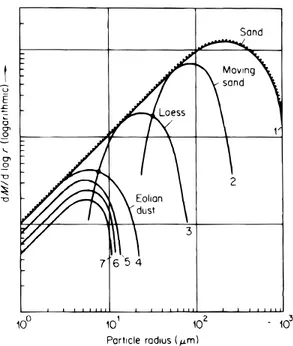
Figure 2.4: Size fractions of sand by wind induced transport, schematic. The original distribution 1 is fractionated into major fractions 2, 3, and 4 as a function of distance from the source. Curves 5, 6, and 7 depict the change in concentration due to both wet and dry removal from the atmosphere. The sum of curves 2, 3, and 4 should be equal to the original curve 1. From [Junge, 1979].

P equals the accumulation A this yields for the particle concentration c_F in the firn:

c_F = F/A = (v_D/A+ε)c_L. This expression may be used to infer v_D and ε from ice core studies if a systematic variation of c_F with A is encountered (e.g. [Fischer et al., 1998; Stanzick, 2001]).

2.5 Size distribution

The size distribution of particulate matter in the source region susceptible to transport during a storm spans a very large range; it reaches from sub-micron to millimeter sized particles (see Figure 2.4). However, as already mentioned in section 2.2 the size range of particles that may remain suspended in the air for considerable time terminates at around 20 to 50 µm diameter. Therefore, the size distribution of the aeolian dust fraction is largely independent from that of the source itself.

Gillette et al. [1974] find that the wind speed has little influence on the size dis- tribution of the airborne fraction in the investigated range from 2-10 µm diameter.

And also D’Almeida and Sch¨utz[1983] observe that dust storms do not change the size distribution of particles aloft below 10µm diameter. Only above 10µm the abundance

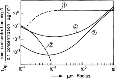
Figure 2.5: Calculated size fractionation due to precipitation. (1) nucleation, (2) at- tachment, (3) below cloud scavenging, (4) dry deposition. From [Junge, 1977].

of large airborne particles increases during strong surface winds. Because here only those particles are considered that are carried long distances the fraction larger than 10 µm may be disregarded. Therefore, it may be assumed that the size distribution of airborne particles a few meters above the ground is independent from the source strength.

Once airborne, the size distribution of an ensemble of particles may be changed by wet and dry deposition. All wet and dry removal processes are size fractionating and therefore modify the size distribution of the remaining particles. As large particles are preferentially removed the size distribution shifts towards smaller particles during long range transport. For the same reason the size distribution is shifted towards larger particles during deposition onto the ice sheet.

The size fractionation of wet removal mechanisms is depicted in Figure 2.5. It shows predictions of the scavenging efficiency depending on particle size for the most important processes. Curve (1) depicts the uptake of aerosols as condensation nuclei.

Curve (2) describes the attachment to cloud droplets by Brownian diffusion and Stefan- flow. (3) is the pick up by falling raindrops (wash-out), and (4) is dry deposition.

Calculations of the dry deposition velocity are shown in Figure 2.6. Deposition is efficient for small particles due to their high diffusivity. Deposition is also high for large particles due to sedimentation; here, the deposition velocity has a slope of 2 in the log- log plot which reflects Stokes law of viscose friction. For intermediate sized particles the deposition is governed by inertial scavenging. This mechanism is influenced by the friction velocity u_∗ and the surface roughness z₀ in a complicated way. As a rule of thumb,u_∗may be taken as a few percent of the average wind speed. z₀ may be taken as

Figure 2.6: Calculated dry deposition velocities at 1 m for u_∗ = 20 cm s⁻¹. From [Sehmel, 1980].

10% to 20% of the physical surface roughness, and a snow surface may be represented by z0 = 0.1 cm [Sehmel, 1980]. Further literature may be found at [Nicholson, 1988;

Wesely and Hicks, 2000].

Both, wet and dry removal processes exhibit a minimal effectiveness in the size range around roughly 1 µm diameter. Therefore, it is not surprising to find the maximum of the mode of aeolian dust carried long distances in this size range. However, as the deposition mechanisms active in this size range are complicated and not very well understood further investigations are clearly needed. This is especially relevant for predictions of size shifts during deposition depending on variable micrometeorological conditions.

Particle counting and sizing

In this chapter a novel laser sensor for microparticle measurements is presented. Its measurement principle and the size calibration are described. Further more, practical laboratory experiences are reported, and the parametrization of the particle size dis- tribution with the lognormal distribution function is discussed. Information on the use and calibration of the laser sensor is also given in the methodical sections of chapters 4 and 5, and in appendix A.

3.1 Measuring techniques for microparticle analy- sis

There are various methods to measure the concentration and size distribution of mi- croparticles in ice cores. Most of these methods use liquid samples; under certain circumstances some of the optical methods described below even work the ice directly.

All methods are either based on single particle detection or on the assessment of the bulk particle content.

Filtration of a liquid sample with consequent microscopy or element analyses is a practiced method. But it is not applied regularly and does not reach a high depth resolution. Further, it only yields either a size distribution or the particle concentration but not both at the same time.

The Coulter Counter method is well established for ice core analyses (e.g. [Petit et al., 1981; Geis, 1988; Steffensen, 1997]); here, single particle volumes are measured in liquid samples. The big advantage of this method is that the volume of the particle is measured independently from its shape. Size distribution and particle concentration are obtained simultaneously and the size range covered is approximately from 0.5µm to

16

20µm diameter, which is appropriate for the analysis of windblown mineral particles in remote regions. The disadvantages of the Coulter method are, however, that extensive sample preparation is required, that the measuring procedure is tedious and that the device is very delicate and susceptible to external disturbances.

Optical methods usually use the intensity of 90^o scattered light to infer the particle concentration. This principle may be applied to individual liquid samples [Hammer, 1977] or using a flow-through setup [Ram and Illing, 1994]. It also works directly on bubble-free ice [Ram and Koenig, 1997]. Very recently, also the successful application of a borehole logger has been reported [Bay et al., 2001]. All these applications may yield a particle concentration, but they do not yield a size distribution. Also, no calibrated high-resolution profiles have yet been published, which indicates calibration problems.

The advantage of these optical methods is the rapidity of the measurement. If the measurement is performed directly on ice only little sample preparation is necessary.

For measurements on liquid samples a continuous flow setup can be used, which al- lows very efficient sample preparation via controlled longitudinal sample melting (see [R¨othlisberger et al., 2000] and appendix B, in German). Here, ice core aliquots of typically 1 m length are continuously melted in a controlled and contamination-free fashion and the work-intensive preparation of individual samples can be omitted. This method enables continuous measurements and a very high depth resolution.

In the work presented here a novel optical measuring technique has been used. It is based on the detection of transmitted rather than scattered light. Like the Coulter method it performs single particle detection and simultaneously yields particle concen- tration and size distribution. Therefore, the efficiency of optical counting may be used without lacking size information.

3.2 The laser sensor: measurement principle and operational parameters

The particle detector was developed by Klotz GmbH, Bad Liebenzell (Germany) for general purpose laboratory applications. For ice core analyses it was specifically modi- fied in a close collaboration ofKlotz and theInstitut f¨ur Umweltpysik of the University of Heidelberg and its applicability was verified by Saey [1998] and Armbruster [2000].

Within the work presented here it was deployed for the first time during a field season.

The device works on a flow-through basis. The sample liquid is pumped through a very small measuring cell of quarz and stainless steel. There, it is illuminated perpen- dicularly to its flow direction by a laser beam with 670 nm wavelength. The measuring

detector laser light

670 nm

1.5 µm

particle

quartz glass window sample flow

Figure 3.1: The detection cell of the laser particle detector.

cell has a cross section of 250µm×230µm (perpendicular to flow direction). The laser beam is only 1.5 µm high but covers the detection cell across its full width. Thus, the surveyed volume is 250µm×230µm×1.5µm (see Figure 3.1). The transmitted light is measured by a photo diode. When a microparticle passes through the laser beam the transmitted light is attenuated by geometric shadowing and scattering processes.

This leads to a negative peak, which is detected and sorted by height into one of up to 32 channels. The channels may be adjusted freely within the size spectrum.

An internal storage can hold accumulated size distribution data, which later may be transferred to a computer for processing. Size distribution data may be accumulated over sample intervals manually controlled by the user or automatically controlled based on a specified time interval or accumulated counts. The device has an analog output which’s voltage is proportional to the momentary count rate. This can be used for high resolution profiling. Essential to the detection method are the dimensions of the laser beam. The very narrow beam strongly enhances the sensitivity of detection by decreasing the steady background signal for the photo diode and reducing the problem of forward scattering.

Coincidence losses may occur at very high count rates due to dead time of the detector electronics after each count; this type of loss would influence the measured concentration but not the size distribution. Coincidence losses due to the simultaneous presence of more than one particle in the surveyed volume would lead to the regis- tration of one large instead of two small particles and therefore alter the measured size distribution; however, coincidence losses of the second type occur very rarely and therefore the size distributions remain intact even if coincidence of the first type should occur.

To ensure a linear conversion of the measured concentration the analog output is

sample

sample water

0.4

4.5 2.0

overflow

particle detector

(A) 2.0

(B)

mixing cell particle detector

Figure 3.2: The dilution setup. Numbers denote flow rates in ml min⁻¹. Samples with moderate or low microparticle concentration could be measured directly (A). Samples with high concentrations were diluted with particle-free carrier water (B).

Parameter Value

min. particle diameter 1.0 µm

optimal flow rate 2 (1.3 - 4.0) ml min⁻¹ max. count rate (analogue output) 4000 s⁻¹

background count rate typ. 2 s⁻¹

Table 3.1: Parameters of the laser sensor. The range given for the optimal flow rate indicates an interval where operation was found appreciable. The maximal count rate is limited due to internal settings of the analog output only (see [Saey, 1998] for details).

limited to a maximum count rate of 4000 s⁻¹. To avoid data loss at high concentration therefore the count rate was reduced by reducing the sample flow rate. However, as low flow rates enhance sample dispersion in the flow system particle-free carrier water was added to the sample in a T-junction. After the two liquid streams were joined the sample was dispersed in a mixing cell of approximately 0.4 ml volume. The mixing improved the homogeneity of the sample at the detector and ensured that the overflow of the mixing cell would not fractionate between sample and carrier water. The dilution setup is sketched in Figure 3.2.

The sample liquid is not contaminated or altered through the measurement and may be further used for other applications (e.g. ion chromatography). The most important parameters of the laser sensor are given in Table 3.1.

3.3 The laser sensor: size calibration

The inter-relation of peak height and particle size is very complex, first because the microparticles are not spherical, and second because detection is based on complicated

optical processes. For large particles with a diameter d ≥ 5 µm geometric shadowing is the most important process [Saey, 1998]; for smaller particles scattering processes become increasingly important (Mie-scattering). For both processes peak height does not only depend on particle volume but also on its geometrical shape, its material (optical density), and on the orientation which the particle randomly has when it passes the laser beam. Considering such a complexity the analytical calculation of the characteristic curve linking peak height with particle size seems hopeless. A good calibration, however, could empirically be achieved via the comparison with Coulter Counter measurements.

For the calibration, several sections of the NGRIP ice core were measured simulta- neously with the lasers sensor and a Coulter Counter. Subsequently the laser sensor data was shifted on the size axis to fit the Coulter Counter data. This is legitimate because the counting efficiencies of the two counters have been shown to be equal [Saey, 1998]. In praxis, the size adjustment was done starting at the upper end of the size spectrum, where the calibration of the laser sensor can independently be achieved through measurements of monodispersed latex spheres of known diameter. Also, the emergence of particle count rates from zero when going from larger to smaller particles can be recognized clearly in both data sets and provides a linkage for the two distribu- tions. Figure 1 on page 69 shows a set of size spectra that were used for the calibration of the NGRIP data. For details see also the description of the calibration in chapter 5 on page 48.

It was noticed, however, that the flow setup may influence the size distribution to an extent not negligible. This effect was especially strong when the dilution setup was in use. Individual calibrations were therefore needed to compensate for the changes of the respective flow setup used. Listings of the calibrations and respective technical details are given in appendix A.

Assessing the accuracy of the calibrations is difficult because there are not many Coulter Counter measurements available for a comparison. However, the modes of lognormal fits of the Coulter Counter or of the laser sensor data differ by typically 0.1 µm as can be seen from Figure 1 on page 69. Since this difference is probably largely due to non-identical sample populations (for explanation see there) it may be inferred that the error of the calibration itself is likely less than 0.1 µm. Double measurements of several samples – one time performed with and one time without the dilution setup – agreed also within 0.1 µm tolerance.

In future applications the laser sensor should again be calibrated via Coulter Counter measurements together with the flow setup used to compensate for the influence of the flow setup. Systematic investigations of the size and the stability of the influence of

20 40 60 80 0.2

0.3 0.4 0.5

Flow rate v (ml min-1 )

Number of runs with same pump tube

Figure 3.3: Change of the flow rate during the lifetime of a pump tube of the NGRIP measurements. Symbols represent flow rate checks. Lines show spline interpolations.

The duration of one particle measurement run is approximately one hour.

the flow setup are desirable to enhance the reliability of the calibrations.

3.4 Determination of flow rates

To calculate the particle number concentration CN not only the total number of counts N but also the associated volumeV of sample liquid needs to be measured. During high resolution profiling the momentary count rate n is recorded and needs to be divided by the flow rate v, as CN =N/V =n/v. Therefore, to infer the particle concentration the flow rate must also be accurately known.

Peristaltic pumps and Tygon pump tubes were used to feed the sample through the particle detector. (See Figure B.3 on page 111 for an example of a flow setup.) These pumps are easy to maintain and cause only little sample dispersion. On the other hand, the flow rates are not constant as the pump tubes deteriorate with regular wear and tear. Therefore, in the course of the measurements during the NGRIP 2000 field campaign all flow rates relevant to the particle measurement were checked daily.

Figure 3.3 illustrates the change of flow rates of various pump tubes. It can be noticed that during the use of a pump tube over several days its flow rate increases by typically

15% and in extreme cases by up to 50%. The difference between two flow rate checks on consecutive days, which spanned usually 15 to 20 particle measurement runs, is typically 5% to 10%.

To assign a flow rate to each particle measurement run the measured flow rates were non-linearly interpolated. The interpolation was based on cubic splines, but it was ensured that no additional local maxima or minima were produced. However, the flow rate was not always measured right after and right before the exchange of a pump tube; in these cases the flow rate data needed to be extrapolated beyond the first and last point of measurement. Hereby it was aimed for an usual development so that the resulting curve fitted well into the existing group. The error of the pump rate assigned to each run after the interpolation performed is estimated to 5%.

In future applications the flow rates should be checked more frequently and es- pecially right before and right after a pump tube is exchanged. An even better im- provement would be the use of a calibrated continuously working flow meter because sometimes conventional flow rate measurements are not feasible even if needed, e.g. if a pump tube unexpectedly breaks down.

3.5 Parameterization of the size spectrum

The lognormal distribution is broadly used for the description of size distribution in aerosol sciences [Davies, 1974; Patterson and Gillette, 1977] and was also adopted to parameterize microparticle size distributions in ice cores, e.g. [Royer et al., 1983;De An- gelis et al., 1984;Wagenbach and Geis, 1989;Steffensen, 1997]. Other approaches such as the empirical law by Junge [Junge, 1963] are not used much any more in this field.

In a new investigation Delmonte et al. [2002] found that size spectra with a very high size resolution are slightly better described with the 4-parameter Weibull than with the 3-parameter lognormal distribution. But the mathematical properties and the physical interpretability of its parameters are strong advantages of the lognormal function. And as the data considered here has only a low size resolution the lognormal distribution can be used without drawbacks.

Mathematics of the lognormal distribution In the following the notation of [Herdan and Smith, 1953] is adopted. Further information can be found in [Cadle, 1955] or [Aitchison and Brown, 1957].

The probability densityp(x) is calledlognormal if q(z) is a normal distribution and

p(x) =q(z) forz = lnx, i.e.

p(x) =A 1

√2πlnσe⁻¹²(^lnx−lnlnσ ^µ)² with:

A: the total integral of the distribution;

µ: the geometric mean of the distribution (here identical with the median), as lnµ= lnx_i = _N^{1 P}lnx_i = ln (^Qx_i)^N1; and

σ: geometrical standard deviation of the distribution, i.e. the standard deviation of ratios about µ, as lnσ=

r

1 N

P ³lnx_i−lnx_i^´2 =

r

1 N

P ³ln^x_µ^i´2.

The probabilityP to find a valuez₀within an interval [a, b] is given byP (z₀ ∈[a, b]) =

Rb

a q(z)dz = ^lnRb

lna

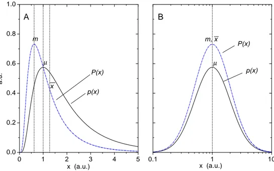
p(x)dlnx. When going from a continuous to a discrete distribution with bins i the probability P_i to find a value in the i-th bin is P_i = p(x_i) (∆ lnx)_i where x_i is a suitably chosen value in the i-th bin and (∆ lnx)_i is the width of this bin on a logarithmic scale. If all bins are equidistantly spaced on a logarithmic scale then all factors (∆ lnx)_i are equal and it is P_i ∝ p(x_i). This means in particular that with a logarithmically-equidistant spacing of bins the most probable value – the so-called mode m, which is the maximum of P(x) – falls together with the maximum (iden- tical with the geometric mean) µ of the density distribution p(x). This situation is illustrated in Figure 3.4-B.

However, if the bin spacings are equidistant on a linear scale then all factors (∆x)_i are equal and using (∆ lnx)_i = ^(∆x)_x ⁱ it is found that P_i ∝ _x¹

ip(x_i). In this case the modem, i.e. the most probable value, is not identical withµbut insteadm=µe^−(lnσ)2. Also the arithmetic mean x is different from m; it is given by x =µe^+12(lnσ)2. This is illustrated in Figure 3.4-A.

Figure 3.4 illustrates the differences between linear (A) and logarithmic (B) bin- (or axis-) spacing. The linear spacing has the advantage that it is area-conservative, i.e. equal areas represent equal probabilities; but the mathematical properties of the linearly spaced distribution are somewhat obscure. The logarithmic spacing on the other hand has the advantages that the full size range may be covered adequately and above all that the mathematical description is easier to grasp because the mode (most probable value), the geometric mean (maximum of the density distribution), and the arithmetic mean all are identical. In the following we will therefore always consider logarithmic densities _dln^dN_d for the size distribution by counts or _d^dV_lnd for the size distribution by volume, andµwill be referred to as the mode. The size distributions shown in chapter 5 in addition are plotted on a logarithmic y-axis to better reproduce the great dynamic range of the distributions; in such log-log-scaling the shape of the

0 1 2 3 4 5 0.0

0.2 0.4 0.6 0.8 1.0

µ x m

P(x) p(x)

a.u.

x (a.u.) x (a.u.)

A

0.1 1 10

µ

m, x P(x)

p(x)

B

Figure 3.4: The lognormal distribution with linear (A) and logarithmic (B) bin- or axis-spacings. Shown is for both cases the probability densityp(x) and the probability P(x) for bins equidistant on the respective axis. Indicated are the most probable value m (the mode, which is the maximum of P(x)), the geometric mean µ (= median), which is the maximum ofp(x), and the arithmetic meanx.

lognormal distribution is parabolical.

The mathematical advantages of the lognormal distribution particularly lie in the properties of its moment-functions. The l-th moment of a probability distributionq(z) is the expectation of z^l, i.e.^R z^lp(z)dz. With the lognormal distribution the lognormal character is preserved when going from the distribution from one moment to that of another. In doing so, the parameters transform as follows:

lnµ7→lnµ⁰ = lnµ+l(lnσ)², i.e. µ⁰ =µe^l(lnσ)2, and lnσ 7→lnσ⁰ = lnσ i.e. σ⁰ =σ.

The meaning of the most important moments are listed in table 3.2 together with their transformation properties. The transformation are of practical relevance e.g. for the transition from a size distribution by number to one by volume, or reverse. First it is remarkable that the distributions by number and by volume may both be lognormal at the same time. Further, the transformation properties are most simple: Given for example the size distribution of particlevolumes with modeµ_V and standard deviation σ_V then the parameters µ_N and σ_N of the size distribution of particle numbers are

l-th Moment Significance lnµ⁰ =. . .

0 d⁰ : number lnµ

1 d¹ : length lnµ+ 1(lnσ)² 2 d² : surface lnµ+ 2(lnσ)² 3 d³ : volume lnµ+ 3(lnσ)²

Table 3.2: Moments of the lognormal distribution and their significance.

obtained through the transformation from the 3rd to the 0th moment:

lnµN = lnµV −3(lnσ)², and σ_N =σ_V.

The reverse transition from the distribution by number to the distribution by volume is obtained correspondingly through the transformation from the 0th to the 3rd moment.

The distribution by surface area may be inferred likewise (see Table 3.2).

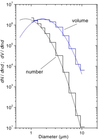
Practical application The size distribution that can be obtained from the laser sensor is in the format of a number distribution. Thereby the size range covered by the detector lies in the upper flank of the number distribution of microparticles and does not include the maximum (the mode). The lack of the maximum in the distribution data leads to higher uncertainties in curve fitting to determine the parameters of the distribution. However, the covered size range includes the maximum of the volume distribution; this provides more rigid boundary conditions for the curve fit and improves the accuracy of the determined parameters. Therefore, the curve fit is performed after the distribution by numbers is transformed to a distribution by volume.

For the transformation of the measured data to a distribution by volume the ac- cumulated counts in each bin are converted to an accumulated volume. To do so a characteristic mean single particle volume vi = ^4π₃ ^³d₂^i´2 is assigned to each bin; in a first approximation the characteristic diameter of each bin is taken as d_i = ^qd⁺_i d⁻_i where d⁺_i and d⁻_i are the upper and lower bin boundary, respectively. In the data considered in this work the bins are chosen rather wide (d⁺/d⁻ ≈1.3); therefore, the size distribution of the data within each bin is accounted for by successive refinements in the choice of d_i. For that purpose d_i is calculated for each bin in a ”next order ap- proximation” from the optimized fit function; then the transformation of the measured data to a volume distribution and the curve fitting are redone using the new values for d_i. This procedure is repeated until no significant corrections of the fit parameters are

1 10 10¹

10² 10³ 10⁴ 10⁵ 10⁶ 10⁷

volume

number

dV / dlnddN / dlnd ;

Diameter (µm)

Figure 3.5: Size distribution by number and by volume. The fit is performed on the volume distribution as it provides more rigid boundary conditions. The modeµ_V was found at 1.68 µm which corresponds to µ_N = 0.87 µm (with σ = 1.66). The data shown is that of a NGRIP sample from the LGM period.

observed (usually after two iterations). The corrections ofd_iyields small improvements to the fit parameters.

The curve fitting is done via parameter optimization using a MATLAB-script based on the Nelder-Mead algorithm. As a measure for the error the relative quadratic error sum between measurement data y_i and model data z_i is taken in the form of

P(lny_i−lnz_i)². This yields better results than considering the absolute errors because the distribution data covers several orders of magnitude in some size spectra, and otherwise the fit would be dominated by a few points close to the maximum.

Figure 3.5 gives an example of the size distribution of a NGRIP sample by number and by volume. The optimized fit curve is included for both forms of the distribution.

It was obtained as described above from the distribution by volume and subsequently transformed to the distribution by number. The data range considered for the curve

fit is from 1.0 µm to 7.5 µm.

High resolution microparticle

profiles at NGRIP: Case studies of the calcium – dust relationship

Urs Ruth, Dietmar Wagenbach, Matthias Bigler, Jørgen P. Steffensen, Regine R¨othlisberger, and Heinz Miller

Annals of Glaciology, Volume 35 (2002), in press

28

case studies of the calcium - dust relationship

Urs Ruth^1,2, Dietmar Wagenbach¹, Matthias Bigler³, Jørgen P. Steffensen⁴, Regine Röthlisberger³, and Heinz Miller²

1Institut für Umweltphysik, University of Heidelberg, Germany

2Alfred Wegener Institut für Polar- und Meeresforschung, Bremerhaven, Germany

3Climate and Environmental Physics, University of Bern, Switzerland

4Department of Geophysics, University of Copenhagen, Denmark

Annals of Glaciology, Volume 35 (2002), in press

ABSTRACT

A novel flow-through microparticle detector was deployed concurrently with continuous flow analyses of major ions during the NGRIP 2000 field season. The easy handling detector performs continuous counting and sizing. In this deployment the lower size detection limit was conservatively set to 1.0 µm equivalent spherical particle diameter, and a depth resolution of ≤ 1 cm was achieved for microparticle concentrations. The dust concentration usually followed the Ca²⁺ variability. Here results are presented from an inspection of the Ca/dust mass ratio in 23 selected intervals, 1.65m long each, covering different climatic periods including Holocene and last glacial maximum (LGM). A (Ca²⁺)/(insoluble dust) mass ratio of 0.29 was found for Holocene and 0.11 for LGM. Changes of the Ca/dust ratio also occur on an annual to multi-annual time scale exhibiting the same pattern, i.e. a lower Ca/dust ratio for higher crustal concentrations. Moreover, the Ca²⁺/dust ratio may increase significantly during episodic events such as volcanic horizons due to enhanced dissolution of CaCO3. This questions the notion of deploying Ca2+ as a quantitative mineral dust reference species and stresses the importance of variable source properties or fractionating processes during transport and deposition.

INTRODUCTION

The atmospheric mineral dust load, mainly composed of insoluble mineral particles, is an important part of Earth’s climatic system as it is involved in direct and indirect radiative forcing processes (e.g. Tegen and Fung, 1994). Equally, the amount, size distribution and composition of dust deposited on polar ice sheets may hold valuable information about both, positions and climatic conditions of source areas, as well as about long range transport and deposition processes (Biscaye and others, 1997;

Fuhrer and others, 1999). Over the last climatic cycle, Greenland as well as Antarctic mineral dust records exhibit changes on a huge dynamic range (e.g. Hansson, 1994;

Steffensen, 1997; Petit and others, 1999). In Greenland these changes occurred very rapidly and were coinciding with changes in δ¹⁸O at rapid climatic transitions within the last Pleistocene as has been inferred from high resolution measurements of Ca²⁺ and ECM on the GRIP and GISP2 ice cores (Taylor and others, 1997; Fuhrer and others, 1999).

The concentration of Ca ions (Ca²⁺) is often being used as a proxy parameter for total mineral dust in ice cores as it represents the major part of the readily dissolved fraction of the dust aerosol. But the soluble proportion of dust is not constant over different climatic periods (Steffensen, 1997), so using Ca²⁺ as a proxy may give a distorted view of the total dust concentration. However, also dust measurement techniques have specific disadvantages. Only low resolution profiles or selected continuous sections have been measured for insoluble microparticles using the well established Coulter counting technique (e.g. Steffensen, 1997) because it requires extensive sample preparation and handling. And high resolution continuous dust measurements using 90° laser light scattering off melt water (Hammer and others, 1985) or off ice (Ram and Koenig, 1997) yield no size distribution information or are difficult to calibrate.

Here we introduce a novel laser sensor device for microparticle measurements deployed for continuous recordings of microparticle concentration and size distribution during the North Greenland Ice Core Project (NGRIP) 2000 field season. Apart from the methodical aspects, we present and discuss case studies of the dust concentration focussing on the Ca²⁺/dust ratio under inconspicuous conditions as well as in volcanic horizons.

EXPERIMENTAL SETUP

During the NGRIP 2000 field season, extensive scientific processing was performed shortly after retrieval of the ice core. This included the operation of a warm laboratory for continuous flow analyses (CFA) of Ca²⁺, Na⁺, NH4+

, SO42-

, NO3-

, H2O2

and HCHO concentrations, and of electrolytical conductivity (Röthlisberger and others,