Working Paper
A synthetic population for the greater São Paulo metropolitan region
Author(s):
Sallard, Aurore; Balać, Miloš; Hörl, Sebastian Publication Date:
2020-08
Permanent Link:
https://doi.org/10.3929/ethz-b-000429951
Rights / License:
In Copyright - Non-Commercial Use Permitted
This page was generated automatically upon download from the ETH Zurich Research Collection. For more information please consult the Terms of use.
ETH Library
Aurore Sallard
IVT, ETH Zürich, 8093 Zürich, Switzerland phone: +41-44-633-38-01
email: aurore.sallard@ivt.baug.ethz.ch orcid: 0000-0001-6465-858X
3
4
Miloš Balać
IVT, ETH Zürich, 8093 Zürich, Switzerland phone: +41-44-633-39-43
email: milos.balac@ivt.baug.ethz.ch orcid: 0000-0002-6099-7442
5
6
Sebastian Hörl
IVT, ETH Zürich, 8093 Zürich, Switzerland phone: +41-44-633-39-43
email: sebastian.hoerl@ivt.baug.ethz.ch orcid: 0000-0002-9018-432X
7
8
Words: 7468 words
9
ABSTRACT
1
This paper presents an open-source generalized pipeline for the creation of a synthetic population
2
for the Greater São Paulo Metropolitan Region, entirely based on open data. The pipeline that is
3
first developed and applied to the Île-de-France region is used as a baseline. Using data-driven
4
algorithms, the pipeline creates a path from raw data to the synthetic population and, further, to the
5
final mobility scenario.
6
A definite advantage of this approach is that it enables to easily reproduce not only synthetic
7
populations, but also to reproduce transportation studies. The São Paulo’s synthetic population, that
8
comprises of as many agents as there are inhabitants in this area, is created using this framework and
9
then analyzed. All considered indicators suggest that this approach is able to model the population
10
on a high level, even if certain gaps could be filled with additional information.
11
INTRODUCTION
1
Agent-based models can represent complex interactions of single entities in large systems. In
2
transportation they are used to model, on a large scale, interactions between individual travelers,
3
their impact on transportation system, and different transportation providers and their operational
4
decisions.
5
Especially recently, agent-based models have gained popularity to simulate human behavior.
6
The main reasons for this are emerging mobility solutions, like shared and on-demand mobility,
7
and dynamically changing demand and supply, which leads to the need for short-term operational
8
decisions. Agent-based models can therefore be a very useful tool to model new mobility solutions
9
and their operational challenge. However, in order to do this, they require substantial input data.
10
This data can be usually separated into transport supply and demand. The core of the transportation
11
demand are individuals that perform activities in the studied area and their activity patterns. In the
12
literature, this demand is usually referred to as the synthetic population with activity chains.
13
This paper presents an open-source approach using only open-data to create the synthetic
14
population with activity chains for the Greater São Paulo Metropolitan Region, the largest urban
15
area in South America and ninth in the world with a population estimate of 21 million inhabitants.
16
This metropolis spreads over a 8 thousand square kilometers area and connects 39 municipalities
17
and is at the center of the São Paulo Macrometropolis, a megalopolis gathering more than 30 million
18
inhabitants. São Paulo is the cultural, economic and financial center of Brazil, representing alone
19
10.7% of the Brazilian gdp.
20
While the main goal of the authors is to use the generated synthetic population as an input to an
21
agent-based model, it can be utilized for other purposes as well. This is achieved by providing the
22
synthetic population in different formats and data frames, which are only later transformed into the
23
necessary format for the use in an agent-based model.
24
The rest of the paper will guide the reader through the open-data used for this work, different
25
stages of the population synthesis pipeline developed in theeqasim framework, and validation
26
results, before concluding with a discussion of the methodology and results.
27
BACKGROUND
28
Aggregated four-step models (Ortuzar and Willumsen (1)) have been used in transportation for
29
decades to assess the impact of new policies or investments. However, they do not consider the
30
individuals’ decisions and their interactions, and do not capture the fact that the demand for travel
31
comes from the necessity to perform activities as it was shown in Chapin (2). This is why the
32
more recent activity-based and agent-based models could be applied successfully in the field of
33
transportation science.
34
Activity-based models (for early reviews, see Kitamura(3), Axhausen and Gärling(4) and Recker
35
(5)) emerged as an answer to the drawbacks of the four-steps models. This approach is based on the
36
work presented in the 70s in Chapin(2) and Hägerstrand(6) —the latter formulating that individual’s
37
activities are limited by social and personal constraints.
38
The activity-based models allow for scheduling activities and making mode and destination choices
1
at the individuals’ scale, within the household context. Several methods, presented in Chu et al.
2
(7), can be applied to synthesize the daily activity patterns. The authors of Wen(8) developed an
3
operational econometric model for generating complex daily patterns, taking interdependencies
4
within households into account and including activity location assignments and travel mode choices.
5
In Lee et al.(9), the Household Travel Survey conducted in the Tucson area in fall 2000 was used and
6
models to better understand the trip chaining behaviors within five different categories of households
7
were constructed. A third approach, featuring the discrete choice models, was proposed in Bowman
8
(10) and in Bowman(11). In those works, the daily activity pattern is seen as a set of tours, each
9
one being characterized by a primary (which means here “most important”) activity. This approach
10
was applied to the Portland area; the results include a synthesized, detailed daily activity pattern for
11
each individual in the population.
12
Unlike the four-step approach, the activity-based models enable insights into various aspects of the
13
results. For instance, with the discrete choice approach from Bowman(10) and in Bowman(11),
14
the results can be aggregated either according to some socio-demographic attribute or at a zonal
15
level. Nevertheless, to achieve this, one needs to estimate and calibrate sophisticated econometric
16
models. Furthermore, the activity-based models have mostly been developed for a small number of
17
regions, making them not easily extendable. Furthermore, they are often not open-source or lack
18
documentation. A notable exception to this is the activity-based model ActivitySim (ActivitySim
19
(12) ), which is an open-source platform for activity-based travel modeling, developed and used by
20
multiple transportation agencies in the USA.
21
On the other side, agent-based models (described in e.g. Bonabeau(13)) are founded on a synthetic
22
population, in which the agents’ attributes reflect the distributions observed in the actual population.
23
For this purpose, several different data sets, that may have been collected at different times, often
24
have to be combined with each other, which requires the utilization of mathematical procedures like
25
the iterative proportional fitting (IPF, see Wong(14) or Norman(15)) or the more recent iterative
26
proportional updating (IPU, see Ye et al.(16)). For instance, ActivitySim is based on PopulationSim,
27
a framework developed by the same teams, which creates a synthetic population from marginal data
28
obtained from the USA census.
29
The agent-based models aim at simulating the agents’ behavior and their competition to access
30
and use transport infrastructures. Such models make it possible to model congestion patterns
31
and interactions between individuals, a characteristic often needed today as several transportation
32
services co-exist and not only compete with each other, but can also be used in a complementary
33
way. Moreover, they allow for modeling highly dynamic services and interactions on a shorter time
34
scale than the one activity-based models can provide. However, here too, the lack of documentation
35
of the processes leading to the creation of the synthetic population make the scenarios often not
36
reproducible, or not verifiable. Furthermore, the data on which those scenarios are based are rarely
37
open-source.
38
In Hörl and Balać (17), the authors provide an integrated and open-source pipeline aiming at
1
generating a synthetic population from raw data. Thanks to its modularity, this framework can
2
be adapted and extended with ease. A first application of this pipeline to Île-de-France, the
3
region around Paris, is described. First, the input data (the national census, two household travel
4
surveys—one regional and one national—, the national tax registry, and a data bank containing all
5
work places, shops and leisure-related places, all of them being open data sets) is presented. Then,
6
the process leading from this raw data to the final synthetic population is documented in detail.
7
Afterwards, an error analysis is performed, setting the theoretical basis to further assessment of the
8
quality of the synthetic population. This pipeline has been applied to other study cases, namely to
9
California (Balać and Hörl(18)) and to Switzerland (Hörl et al.(19)) – this last scenario being an
10
exception as it is not based on open data.
11
This paper will present another use case of theeqasimframework presented in Hörl and Balać(17).
12
As in the Île-de-France scenario, all the data that are used here are open-source. The goal of the
13
paper is to present a way to create a synthetic population of Sao Paulo region, from raw open-data,
14
with minimal calibration effort that can be used for further behavioral, socio-demographic and
15
transportation analysis.
16
INPUT DATA
17
Input data are the essence of each agent-based scenario. It can be divided into two categories, the
18
first one representing thetransport supplyin the study area, while the second focuses onmobility
19
demand. In the context of this paper, the emphasis will be placed on the mobility demand.
20
The demand is comprised of asynthesized population, namely a set ofagentscharacterized by their
21
attributesand theirplans. A plan is an activity chain describing an agent’s typical schedule during
22
an average working day. It also contains information on the desired times and locations at which the
23
agent wishes to perform those activities and on the trips linking one activity to the following. The
24
attributes describe the socioeconomic condition of the agents and provide information on transport
25
modes that they can access. Agents are grouped intohouseholds, that are themselves characterized
26
by certain attributes.
27
The transport supply consists typically of a street and public transport network. Information
28
concerning transit schedules are required as well, and it is necessary to supplement the road network
29
withfacilitylocalizations, a facility being a place where an agent can perform an activity.
30
In this section, the different sources that were used in the context of the creation of the synthetic
31
population for the Greater São Paulo Metropolitan Region will be presented.
32
Zonal system
33
Figure 3 shows the extent of the study area, which corresponds to the administrative borders of the
34
Greater São Paulo Metropolitan Region – in spite of its contribution to the traffic flows in the study
35
area, the city of Santos could not be included in the model because the household travel survey data
36
does not cover this area. Despite its proximity to the Atlantic Ocean, Sao Paulo is located on a
1
plateau with an average elevation of about 800 meters above the sea level.
2
The study area was divided in 633 zones depicted in Figure 1. This zonal system is the one that
3
was used in the census (which will be described in the next sub-section). This zonal system has
4
been used since the 70s and reviewed regularly. It divides the territory into zones according to
5
geographical characteristics, such as population density, concentration of activities and presence
6
of historical monuments and natural spaces. Moreover, this system ensures a rather homogeneous
7
distribution of the population among the zones: in each one of them, the number of residents is
8
between 20 000 and 55 000.
9
Facility locations
10
Facility locations (including homes, work, shops and leisure-related places) were retrieved from
11
Open Street Maps(20)(osm).
12
In neighborhoods where no home place could be found through osm, home locations were assigned
13
alongside the residential or living streets. Moreover, as OSM data lacks a substantial number of
14
educational places in the study area, a data set from the São Paulo’s Ministry of Education, “Dados
15
Abertos da Educação”(21), was employed to fill this gap. This data set contains in particular the
16
geographical coordinates of all education places in the state of São Paulo, but the level of offered
17
education is unfortunately missing.
18
Mobility demand – the population
19
Two main data sources were used as inputs to create the population. The first one is a census
20
conducted in 2010 in Brazil(22). After removing all samples that had a home place outside the
21
São Paulo State, 3 622 779 weighted samples remained. For each of them, information is provided
22
on the individual’s age, gender, personal income, employment and/or student status. Plenty of
23
other attributes are available, but they were not used in the present study. One has as well access
24
to household related attributes such as total household income, car and motorcycle availability,
25
number of household members and municipality and area codes of the residence place. Among
26
those individuals, 1 211 311 live in the study area and their weights sum up to 19 918 293, which is
27
approximately the total number of inhabitants in the Greater São Paulo Metropolitan Region at the
28
time the survey was conducted. This census is necessary to make sure that the attributes distribution
29
(whether individual or household related) in the synthesized population reflect accurately the real
30
ones. Moreover, it shows the diversity of São Paulo’s population. Figure 1 depicts for instance the
31
average (weighted) personal income per administrative zone in the study area, which is computed
32
as the total household income divided by the number of individuals in the household. The wealth
33
inequalities are obvious: in the most peripheral neighborhoods, the average personal income appears
34
to be lesser than 1 000 BRL (as of January 2020, the minimal legal salary in São Paulo is 1 163
35
BRL; 1 BRL is equivalent to 0.18 USD or 0.17 EUR (exchange rate accessed on May, 6th 2020)).
36
whereas it can reach more than 6 000 BRL in the most central districts.
37
FIGURE 1 Average personal income, computed from the weighted household income, de- pending on the residence administrative zone, in BRL.
Background map ©OpenStreetMap contributors
The second data source was the household travel survey (hts) conducted in the Greater São Paulo
1
Metropolitan Region in 2017(23). It contains 84 889 samples which are weighted, so that the total
2
weight sum amounts to 20 508 979, more or less the number of inhabitants in the area in 2017. For
3
each sample, not only individual attributes are provided, namely age, gender, personal income and
4
employment status, but also information related to the household – household income and number
5
of available cars and bikes for instance. The most important part of the survey are the travel diaries
6
of interviewed individual. They enable to track each individual’s schedule during an average work
7
day. Each entry in the data set corresponds to a trip linking two given activities, which take place
8
at locations known at the coordinate level. Moreover, one has access to the trips characteristics:
9
departure and arrival time and chosen mode. Some sample individuals also answered questions
10
about the parking type they parked in and how much they paid for it. However, those persons were
11
too few to make a further use of this information possible.
12
Origin–Destination matrices
13
An origin–destination matrix is a matrix in which each cell represents the number of trips from an
14
origin zone (given by the corresponding row of the matrix) to a destination zone (column), or the
15
percentage of trips starting in the origin zone that reach the destination zone. Those matrices can be
1
created from the household travel survey. In this study, one weighted origin–destination matrix was
2
generated for work trips.
3
CREATION OF A SYNTHESIZED POPULATION
4
The goal of this section is to present the process leading towards the creation of a synthesised
5
population using the data presented in the previous chapter. The main steps of this process are
6
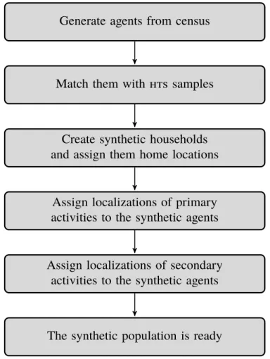
summarized in Figure 2. The pipeline is available as a public GitHub repository(24). Apart from
7
the framework generating the synthetic population that will be described below, this repository
8
also provides scripts embedding this population synthesis into a transport simulation realized with
9
MATSim ((25)) using discrete-mode choice extension(26).
10
Generate agents from census
Match them with hts samples
Create synthetic households and assign them home locations
Assign localizations of primary activities to the synthetic agents
Assign localizations of secondary activities to the synthetic agents
The synthetic population is ready
FIGURE 2 Overview of the population synthesis
The first step is to pre-process the input data in order to keep only relevant persons and trips.
11
After the synthesized agents and households are created from census, that are matched to the hts
12
individuals according a number of attributes. Those agents are then assigned to a specific home
13
location. Finally, the agents’ plans are finalized with the imputation of activity locations.
14
Pre-processing the input data
1
While most of the data sets are used in their original form, some of the information from the hts
2
needed to be adapted to reduce complexity. These adaptations are presented in what follows.
3
Employment, transport mode and trip purpose categories
4
In the hts, respondents were allowed to choose among many different transportation modes. In
5
order to simplify the modeling tasks, they were all merged to eight modes, namely public transport,
6
car, car passenger, walk, bike, taxi and ride-hailing.
7
Similarly, the trip purposes – or activities done at the trip destination – were merged into six
8
categories (home, work, shopping, leisure, education, and other). It has to be noticed that trips done
9
by non studying adults to escort their children from or to school were considered as “education´´
10
trips in the original data set. Those activities were changed to “other´´ to allow for a better reliability
11
of the activity chains prevalence in the output data.
12
With regard to the socio-demographic attributes, it was also decided to reduce the number of
13
employment categories from eight to three —employed, not employed and student.
14
Comparing hts with census employment numbers presented a large disparity in the number of
15
unemployed. The hts contains an additional variable about current school enrollment. Therefore,
16
we performed a check whether those going to school are classified as students. While a substantial
17
number is classified as student, there are some individuals that were classified as either ’jobless’ or
18
’has never worked’. For these, we changed the status of their employment to “student”. As a result,
19
the respective shares of students, employed and unemployed individuals in the hts are closer to the
20
one observed in the census, as Figure 5, page 12, shows.
21
Adding information on residence area
22
One’s mobility patterns are also influenced by one’s residential environment. For instance, in less
23
densely inhabited zones, a trip tends to be longer than in a highly populated neighborhood and the
24
car prevalence tends to decrease in the most urbanized areas, mostly due to difficulties of finding
25
(affordable) parking. It was decided to capture this phenomenon by creating a new attribute, which
26
splits all individual samples from the census and the household travel survey into three groups
27
depending on the location of their home. The Figure 3 shows the three zones that were defined. As
28
the figure shows, a pure geographical definition of those three zones was chosen. One could easily
29
replace this zones by new ones defined by a different criteria easily within the pipeline.
30
Creating synthetic households
31
After cleaning the census and the household travel survey, it is possible to create synthesized agents
32
by directly expanding census data according to their weights. As census is anonymized by only
33
providing a home zone location, further assignment of the exact home location is conducted later in
34
the pipeline. In the next step, each sampled individual is then matched to an observation from the
35
household travel survey, using hot-deck matching ((27),(17)).
36
The idea is to find all source observations (i.e. all samples from the household travel survey)
37
FIGURE 3 The three residential areas defined in the Greater São Paulo Metropolitan Re- gion. The red, inner zone corresponds to the city center of São Paulo; the orange one to the administrative borders of the City of São Paulo and the yellow zone to the rest of the district.
Background map ©OpenStreetMap contributors
that match the target observations (i.e. synthetic agents previously sampled from the census) on a
1
list of given matching attributes, and then to sample randomly one of those source observations.
2
To avoid over-fitting, if too few source observations are found for a given target observation, some
3
matching attributes are removed to enhance the set of matching source observations.
4
The attributes that are taken into account to perform matching are age class, gender, employment
5
status and availability of a car inside the household. In addition, observations that are similar with
6
respect to the residence area (as defined in subsubsection 5.1.2) are preferred.
7
Imputing primary locations
8
Once the agents have been assigned a daily plan based on the household travel survey, a location for
9
each of their primary activities (home, work and education) has to be defined. The aim of this step is
10
twofold: First, a correct number of agents should commute from one zone to another; Secondly, the
11
commute distances should fit the activity chains that have been assigned to the agents in the previous
12
step. While only an overview of the algorithms will be given here, more details can be found in(17).
13
Imputing home locations
14
The next step consists of assigning each synthesized household to a home location. The administrative
15
zone in which each agent lives is known from the census and thus, as all admissible home locations
16
are available from the facility locations database, it is quite straightforward to impute a home place
1
to each synthesized household or agent by selecting randomly a home place among all available
2
locations.
3
Imputing work locations
4
Once the agents are assigned a home location, one can provide them with work locations, if they do
5
have a work-related trip registered in their activity chain. For this purpose, the Origin-Destination
6
(od) matrices are used.
7
Given the residence district of an agent, their workplace district is sampled from the corresponding
8
line of the weighted od matrix. Then, once one knows, for each pair of districts(k,k0), the exact
9
number of agents living in the zonek and commuting to the zonek0, a number denoted by fk,k0, one
10
can sample fk,k0 exact destinations from the data set containing all available work places in the zone
11
k0. The coordinates set resulting from this step is denoted byCk,k0. Those coordinates sets are then
12
aggregated by home districtk: Ck :=Ð
k0Ck,k0.
13
The last step consists of finding a bijective function such that each personuis mapped to the
14
coordinates of a work placec ∈ Ck, such that the distance between the agent’s home and their work
15
place corresponds to the commute distance found in the household travel survey. If there is no direct
16
trip between home and work places in the household travel survey, a random distance is drawn from
17
the commute distances found in this survey.
18
Imputing education locations
19
The imputation of the education locations followed a different way. For the less dense districts, too
20
few observations were registered, which lead to biased od matrices. Moreover, the facility data sets
21
obtained from the Ministry of Education did not provide enough information about the category
22
of education facility (kindergarten, primary or high school or university). Another method was
23
therefore implemented.
24
All education-related trips from the household travel survey were first split into several groups
25
depending first on the residence area type (see subsubsection 5.1.2) the agent lives in, secondly, on
26
the agent’s gender, and, thirdly, on the age of the individual sample who made the trip (and thus
27
on the category of education facility the individual visited: pre-school or elementary school for
28
children aged 14 or less, high school or technical school for teenagers aged 14 to 18, university for
29
people aged 18 to 30 and various places for agents aged 30 or more. For each of these groups, it was
30
then possible to construct the histogram of the distances separating the education place to the home
31
of the individual samples. Finally, a probability density function corresponding to each histogram
32
was obtained.
33
For each agent, a target distance was drawn from the probability function related to the group
34
(age and type of residence area) the agent belongs to. Using a bi-dimensionalk-d tree, an education
35
place was then selected such that the distance separating it from the agent’s home location was as
36
near to the target distance as possible.
37
Imputing secondary locations
1
The imputation of secondary locations, which means places in which leisure, shopping or other
2
activities are performed, is taken over by a method described in(28)or, more briefly, in(17). Here,
3
only a basic idea will be given, so as to provide the reader with some intuition on the employed
4
algorithm.
5
While primary activities (home, work or education) have fixed locations, which were determined
6
in the previous paragraphs, secondary activities (shopping, leisure and other) are not assigned
7
particular locations. The activity chains can be split into smaller chains, in which two fixed activities,
8
the first and last ones, are separated only by various assignable activities. From the household travel
9
survey, one knows ideally how long the trips of each sub-chain should be.
10
First, all trips present in the household travel survey are divided into bins of modes and travel
11
times. Then, given the transport mode and the ideal travel time of each trip that have to be assigned a
12
location, a distance is sampled from the bins previously created. Afterwards, a gravity model is used
13
to assign the variable activities to some locations, defined by coordinates, such that the observed
14
distances resemble the sample. Finally, the closest facility of the target activity type is selected from
15
the facility data sets (for instance, if an agent has to go "shopping", the sampled coordinates will be
16
snapped to the nearest available shop).
17
INSIGHT INTO THE SYNTHESIZED POPULATION
18
The process described above enabled the creation of a synthesized population, in which the agents
19
have been given activity chains obtained from the household travel survey and where those activities
20
are performed in places drawn with various sampling methods from the facility databases.
21
The fact that the census is very accurate, and that the synthetic agents and households are
22
directly sampled from this data set lead to the direct conclusion that a validation step to assess the
23
accuracy of the socio-demographic attributes distribution in the synthesized population is actually
24
not necessary. This is why this point will not be addressed below.
25
Comparison of the activity chains in the synthesized and actual populations
26
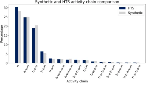
The Figure 4, page 12, shows the distribution of activity chains in the synthesized population and
27
compares it to the observed distribution obtained from the household travel survey.
28
This graph suggests that the synthesis process was quite accurate: the activity chains are present
29
in the correct order and the observed differences between the actual population and the synthesized
30
one are always lower than two percentage points.
31
It can however be seen that chains containing at least one “work” activity (like"h-w-h"or
32
"h-w-l-w-h"in Figure 4) are more frequent in the synthesized population than in the survey
33
population in hts. The reason for this is that the two surveys that were employed for this study were
34
not conducted in the same year. Indeed, the population distribution among the three employment
35
categories – namely “employed”, “unemployed” (which includes retired people as well) and “student”
36
– changed during the seven years separating the time when the census was conducted (in 2010) and
37
the period at which the household travel survey was realized (in 2017). This is what shows Figure 5.
38
FIGURE 4 Activity chains comparison.
hstands for “home”,wfor “work”,efor “education”,lfor “leisure”,sfor “shopping”
andofor “other”.
FIGURE 5 Distribution among employed, unemployed and currently studying persons in the census and in the household travel survey
The employment rate as well as the percentage of students in the population dropped between
1
2010 and 2017. This is why, as the comparison is performed between the synthesized population
2
– sampled from the census conducted in 2010 – and the activity chains present in the household
3
travel survey of 2017 – when the unemployment rate had increased – the plans containing one or
4
more work or education activities are slightly over-represented. Moreover, for the same reason, the
5
number of agents that do not leave their home (those whose activity chain is only"h") tends to
6
be higher in the household travel survey than in the census, and, thus, in the synthetic population.
7
Official sources confirm the quite dramatic raise of unemployment in São Paulo: the unemployment
8
rate was actually around 7% in 2010 (Instituto Brasileiro de Geografia e Estatística(29)) in the
9
metropolis, and increased to 13.4% in 2017 (Instituto Brasileiro de Geografia e Estatística(30)).
10
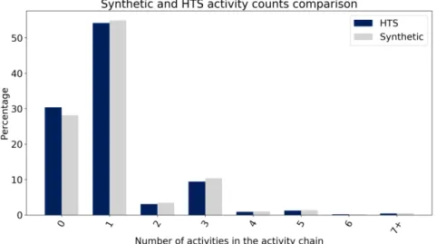
Number of activities in the activity chains and per purpose
1
It could be of interest to have a look at the number of activities performed by the agents. This is
2
what Figure 6, page 13 shows. A number of activities equal to zero means that the agent did not
3
conduct any trip during the day; otherwise, this number was computed by excluding the starting and
4
ending “home” activity. For instance, it was considered that the chain"h-w-h-o-l-h"has four
5
activities.
6
FIGURE 6 Comparison of the number of activities in the agent’s activity chains between the hts and the synthetic population
It can be observed that the relative prevalence order of the activity counts is well respected in
7
the synthetic population. Furthermore, this order makes sense in itself: the major part of the agents
8
(around 55%) has only one activity, namely work or education for the majority of them. Then follow
9
agents with no activity, which is consistent with Figure 4, then agents with 3 activities—a great
10
number of them are working or studying and have their lunch at home. The other activity numbers
11
are much less represented.
12
Those observations are consistent with Figure 7, that shows the prevalence of activity counts per
13
purpose in the synthetic population and compares it to the hts.
14
Comparison of the distance distribution in the synthesized and actual populations
15
Comparing how far agents have to travel to perform a given activity with what is observed in reality
16
will provide helpful evidence of the efficiency of the stages where facility locations are imputed to
17
them. The results of this comparison are presented in Figure 8.
18
When looking at Figure 8(b), it can be noticed that the distance distributions fit reasonably well.
19
Regarding the average distances, the results are satisfactory as well.
20
Comparison of travel purposes and distances between male and female agents
21
As described in the previous section, the activity chains present in the hts are correlated with
22
the sociodemographic attributes of the interviewees and, thanks to the matching process, those
23
FIGURE 7 Comparison of the number of activities per purpose in the agent’s activity chains between the hts and the synthetic population.
Interpretation: both in the hts and in the synthetic population, around 33% of the agents go to work once in the day, while 6% go twice to work.
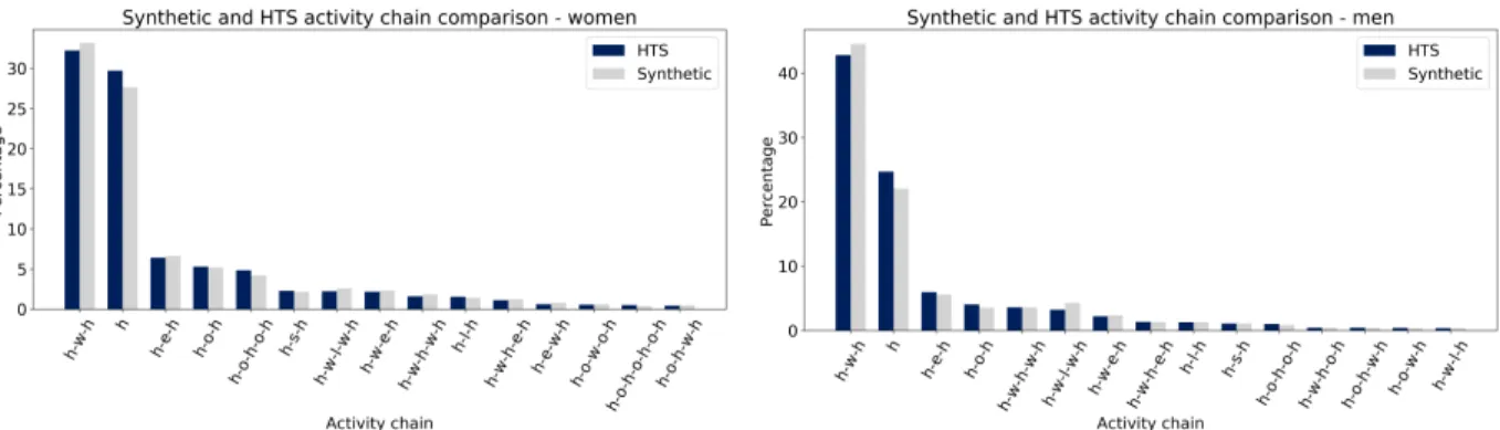
chains are distributed in a meaningful way among the synthetic agents. The Figure 9 compares the
1
prevalence of the most frequent activity chains in the hts and the synthetic population for male
2
and female agents between 18 and 40 years old. The figure shows that the chainh-w-h(going
3
from home to work and then back home) is the most prevalent for both agents groups, but, in the
4
hts as well as in the synthetic population, the observed frequency among males is more than 10
5
percentage points above the frequency observed among female agents (42-45 % versus 55-57%). As
6
a consequence, the chain distribution observed for women seems to be slightly more heavy-tailed
7
than the one characterizing men.
8
This indicates a larger variety of activity patterns for women, a phenomenon that have already
9
been investigated in(31).This observation is confirmed by Figure 10, page 16, that shows the number
10
of activities in the hts and the synthetic population for male and female agents between 18 and 40
11
years old, and by Figure 11, page 16, that illustrates the number of activities per purpose in the same
12
population.
13
It can also be noticed that the fifth most prevalent activity chain is different between the male and
14
the female population: it is indeed“h-w-h-w-h”for men and“h-o-h-o-h”. A further analysis
15
reveals that this chain was originally“h-e-h-e-h”for women; those “education” activities were
16
changed into “other” ones during the cleaning part — some agents, that are not studying, were
17
assigned activity chains with education-related trips if they escorted their children to school. This
18
difference in the activity chain distribution among men and women thus reflects an activity splitting
19
among household members: women who stay at home, take care of the children, whereas men are
20
more often employed and some of them return home for lunch.
21
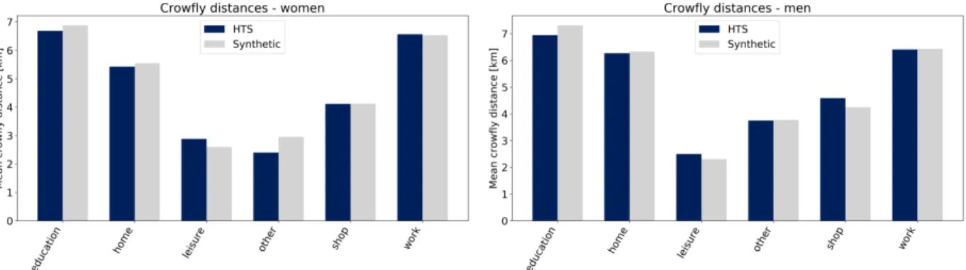
The Figure 12 compares the average travelled distances for different purposes in the same
22
population. As well as before, it can be seen that the reference distributions, obtained from the hts,
23
are well reflected by the synthetic population.
24
(a) Average distances
(b) Distance cumulative distributions FIGURE 8 Crowfly distances towards a facility by activity purpose
Whereas the travelled distances are, on average, similar between men and women, it can be
1
observed that men travel on average 1 to 1.5 more kilometers than women if they travel to an
2
educational place. The travelled distance to home is impacted by this phenomenon—it amounts to
3
around 5.8 km for women and to more than 6 km for men. This would mean that women tend to
4
make more trips related to education, but that the places where they study is located nearer to their
5
homes than they are for men.
6
Comparison of distance from home to the education facility
7
As a special attention was paid to the imputation of education facilities to students and pupils, it
8
was decided to look into the resulting distribution of distances between an agent’s home and the
9
education place they were assigned to. This is shown in Figure 13.
10
(a) Most frequent activity chains among female agents (b) Most frequent activity chains among male agents
FIGURE 9 Most frequent activity chains, comparison between the hts and the synthetic population, split between men and women aged 18 to 40.
(a) Female agents (b) Male agents
FIGURE 10 Number of activities in the chains, comparison between the hts and the syn- thetic population, split between men and women aged 18 to 40.
(a) Female agents (b) Male agents
FIGURE 11 Number of activities per purpose, comparison between the hts and the syn- thetic population, split between men and women aged 18 to 40.
(a) Average travelled distances by female agents (b) Average travelled distances by male agents
FIGURE 12 Average travelled distances, comparison between the hts and the synthetic population, split between men and women aged 18 to 40.
- age.png
FIGURE 13 Comparison of the average distance between an agent’s home and the education place they were assigned to, according to the agent’s age and in the entire population
From the figure, it is clear that the gap between the distances obtained from the hts and the one
1
observed in the synthetic population is small, but one can observe that it increases with the age of
1
the agents. This is linked to the fact that, for instance, there are many more samples of kids aged 14
2
or less going to school than of students aged 25 and more, so the facility sampling process could not
3
achieve the same level of accuracy for all age groups.
4
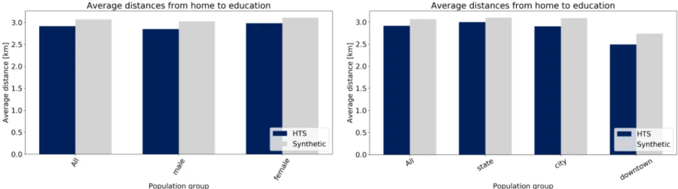
Figure 14(a) and Figure 14(b) show the average distances between home and education facility
5
for agents, according to their gender and category of residence area, as those were the two other
6
factors taken into account during the sampling process.
7
With gaps always smaller than 200 meters for target distances around 3 km, it can be concluded
8
that the approach used for assigning education facilities to students was successful.
9
(a) Average distances according to the agent’s gender (b) Average distances according to the agent’s resi- dence area. “Downtown” designates the agents living in the central area of São Paulo, “city” those who live in the city but not in the downtown, and “state” those living in other parts of the study area, according to the zones defined in subsubsec- tion 5.1.2
FIGURE 14 Comparison of the average distance between an agent’s home and the education place they were assigned to, according to the agent’s gender or residence area and in the entire population
DISCUSSION
1
While the generated synthetic population matches quite well the reference data, some of the observed
2
discrepancies and limitation have to be pointed out.
3
Input data
4
The available input surveys (the census and the household travel survey, conducted respectively
5
in 2010 and 2017), were not carried out the same year and, during the time span separating them,
6
the population structure evolved in many aspects. The unemployment rate in Brazil rose by four
7
percentage points between 2010 and 2017(32)and the observed mobility patterns were influenced
8
by the last developments of the public transport network (like the construction of new metro lines
9
(33)or the start of operations of famous ride-hailing platforms, like Uber in June 2014 as reported
10
in(34)).
11
The population was thus synthesized from two distinct populations and this is why its observed
12
mobility patterns sometimes do not match exactly the ones that were taken as a reference. This can
13
explain most of the differences observed in the previous section.
14
Moreover, the household travel survey only allows to model local personal trips: for instance,
15
neither freight nor tourism are taken into account in the presented approach, due to the lack of data.
16
Imputing categories to facilities
17
A few issues have arisen concerning the creation of the facility data sets. Open Street Map has
18
a poor representation of educational places and the data gathered by the Brazilian Ministry of
19
Education does not separate education places into kindergartens, primary and high schools and
1
universities. Therefore, the first attempts to assign education places to the synthesized agents ended
2
up being erroneous: the distribution of the distances that the agents cover to reach their study
3
location starting from their home was too dissimilar to the targeted distribution. As presented in
4
section 5, the proposed solution was to differentiate those distributions according to the agents’ age;
5
in this way, it ensures the distributions being respected but no guarantee can be offered that each
6
agent is actually linked to an education facility matching his or her age.
7
Further improvements
8
As pointed out in the previous pages, there is still room for improvement which would lead to
9
more accurate results and a better representation of the average mobility demand in the São Paulo
10
Metropolitan Region. Most of it has to do strongly on the data availability:
11
• As mentioned in the introduction, Santos is a major city with a population of more than 400
12
000 inhabitants. As home to the largest seaport of Latin America, located only 80 km away
13
from São Paulo, it is obvious that it contributes to the observed transport flows in the megacity.
14
In particular, taking in account commuter flows from one city to the other would enhance the
15
travel survey and, as a result, improve the quality of the modeled transport demand.
16
• Freight traffic as well as commercial agents’ routes are missing as well in the current trips
17
data sets. As the impact of such trips may not be negligible on the global transport situation,
18
taking them into account would benefit later transport simulation.
19
• Currently, in the process of matching activity chains to individuals, household structure is not
20
considered. As all household members are interviewed in the Household Travel Survey, it
21
would however be possible to maintain the interactions existing within the households in the
22
matching phase. This would ensure, first, that joint trips are modeled properly and, secondly,
23
that shared resources (cars or bicycles, for instance) are distributed appropriately among the
24
household members. For example, this would guarantee that, if an adult member leaves home
25
with the only car available to the household, then no other member can take the car to go
26
shopping before the first one is back.
27
CONCLUSION
28
This paper presented a process to generate a synthetic population for São Paulo based on a new
29
pipeline allowing, among others, to obtain an operational scenario directly from raw data. All the
30
data sets utilized here as well as the framework itself are open-source, and, consequently, if access
31
to raw data is provided, the results are entirely reproducible by others.
32
The proposed approach, based on rather simple algorithms, can be easily adapted to the generation
33
of other scenarios. It could therefore serve as a benchmark for future improvements. It also shows
34
that reliable outputs can be obtained even if the input data is not the most suitable—in the case at
35
hand, the census data was collected seven years before the household travel survey was conducted.
36
Different parts in the article indicate potential future work. Taking into account other variables,
37
such as parking costs, freight traffic or commuter flows from and to the neighboring city of Santos,
38
or considering household structure during the process of matching activity chains to individuals are
1
possible improvement axes. The hope is to continue to collect data to improve the quality of the
2
results and, furthermore, to expand this open-source and open data approach to new scenarios.
3
ACKNOWLEDGMENT
4
We would like to acknowledgeAirbus Urban Mobility GmbHwhose funding has supported the
5
development of a synthetic agent-based scenario for the Greater São Paulo Metropolitan Region.
6
AUTHOR CONTRIBUTION
7
The authors confirm contribution to the paper as follows: study conception and design: A. Sallard,
8
M. Balać, S. Hörl; data collection: A. Sallard, M. Balać; analysis and interpretation of results: A.
9
Sallard, M. Balać; draft manuscript preparation: A. Sallard, M. Balać. All authors reviewed the
10
results and approved the final version of the manuscript.
11
REFERENCES
12
1. Ortuzar, J. and L. Willumsen (2011) Modelling Transport, 4th edition.
13
2. Chapin, F. S. (1974)Human activity patterns in the city: Things people do in time and in space,
14
vol. 13, Wiley-Interscience.
15
3. Kitamura, R. (1988) An evaluation of activity-based travel analysis,Transportation 15, 9–34.
16
4. Axhausen, K. and T. Gärling (1992) Activity-based approaches to travel analysis: conceptual
17
frameworks,models, and research problems,Transport reviews 12, 323–341.
18
5. Recker, W. (1995) The household activity pattern problem: general formulation and solution,
19
Transportation Research Part B: Methodological 29, 61–77.
20
6. Hägerstrand, T. (1970) What about people in regional science?, paper presented at thePapers of
21
the Regional Science Association, vol. 24.
22
7. Chu, Z., L. Cheng and H. Chen (2012) A review of activity-based travel demand modeling, in
23
CICTP 2012: Multimodal Transportation Systems—Convenient, Safe, Cost-Effective, Efficient,
24
48–59.
25
8. Wen, C.-H. (1998) Development of stop generation and tour formation models for the analysis
26
of travel/activity behavior.
27
9. Lee, Y., M. Hickman and S. Washington (2007) Household types and structure, time-use pattern,
28
and trip-chaining behavior, Transportation Research Part A: Policy and Practice, 41 (10)
29
1004–1020.
30
10. Bowman, J. L. (1995) Activity based travel demand model system with daily activity schedules,
31
Ph.D. Thesis, Massachusetts Institute of Technology.
32
11. Bowman, J. L. (1998) The day activity schedule approach to travel demand analysis, Ph.D.
1
Thesis, Massachusetts Institute of Technology.
2
12. ActivitySim (2020) An open platform for activity-based travel modeling, https://
3
activitysim.github.io/.
4
13. Bonabeau, E. (2002) Agent-based modeling: Methods and techniques for simulating human
5
systems,Proceedings of the National Academy of Sciences 99, 7280–7287.
6
14. Wong, D. W. (1992) The reliability of using the iterative proportional fitting procedure,The
7
Professional Geographer,44(3) 340–348.
8
15. Norman, P. (1999) Putting iterative proportional fitting on the researcher’s desk.
9
16. Ye, X., K. Konduri, R. M. Pendyala, B. Sana and P. Waddell (2009) A methodology to match
10
distributions of both household and person attributes in the generation of synthetic populations,
11
paper presented at the88th Annual Meeting of the Transportation Research Board, Washington,
12
DC.
13
17. Hörl, S. and M. Balać (2020) Reproducible scenarios for agent-based transport simulation: A
14
case study for Paris and Île-de-France, May 2020.
15
18. Balać, M. and S. Hörl (2020) Synthetic population for the state of California based on open-data:
16
examples of san francisco bay area and san diego county. Submitted for presentation at TRB
17
2021.
18
19. Hörl, S., F. Becker, T. Dubernet and K. Axhausen (2019) Induzierter Verkehr durch autonome
19
Fahrzeuge: Eine Abschätzung (traffic induced by autonomous vehicles: an estimation),SVI
20
2016/001, Schriftenreihe 1650.
21
20. OpenStreetMap contributors (2017) Planet dump retrieved from https://planet.osm.org ,
22
https://www.openstreetmap.org .
23
21. Coordenadoria de Informação, Evidência, Tecnologia e Matrícula (CITEM) (2020) En-
24
dereços de escolas (addresses of the schools), https://dados.educacao.sp.gov.
25
br/dataset/endereços-de-escolas.
26
22. Instituto Brasileiro de Geografia e Estatística (2011) The 2010 population census sum-
27
mary, https://www.ibge.gov.br/en/statistics/social/population/
28
18391-2010-population-census.html?edicao=19720&t=publicacoes.
29
23. Transportes Metropolitanos (2017) Resultados finais da pesquisa origem e destino 2017
30
(final results of the 2017 origin-destination survey),http://www.metro.sp.gov.br/
31
pesquisa-od/.
32
24. Balać, M. and S. Hörl (2020) Eqasim,https://eqasim.org/.
33
25. Horni, A., K. Nagel and K. W. Axhausen (2016)The Multi-Agent Transport Simulation MATSim,
34
Ubiquity Press, London.
35
26. Hörl, S., M. Balać and K. W. Axhausen (2018) A first look at bridging discrete choice modeling
1
and agent-based microsimulation in MATSim,Procedia computer science,130, 900–907.
2
27. D’Orazio, M., M. Di Zio and M. Scanu (2012) Statistical matching of data from complex sample
3
surveys, paper presented at theProceedings of the European Conference on Quality in Official
4
Statistics-Q2012, vol. 29.
5
28. Hörl, S. and K. W. Axhausen (2020) Relaxation-discretization algorithm for spatially constrained
6
secondary location assignment, paper presented at the99th Annual Meeting of the Transportation
7
Research Board.
8
29. Instituto Brasileiro de Geografia e Estatística (2016) Principais destaques da evolução do
9
mercado de trabalho nas regiões metropolitanas abrangidas pela pesquisa (Main highlights of
10
the evolution of the labor market in the metropolitan regions covered by the survey), ftp:
11
//ftp.ibge.gov.br/Trabalho_e_Rendimento/Pesquisa_Mensal_de_
12
Emprego/Evolucao_Mercado_Trabalho/retrospectiva2003_2011.pdf.
13
30. Instituto Brasileiro de Geografia e Estatística (2017) Pesquisa nacional por amostra de domicílios
14
contínua — quarto trimestre de 2017 (national household sample survey — fourth quar-
15
ter 2017), https://biblioteca.ibge.gov.br/visualizacao/periodicos/
16
2421/pnact_2017_4tri.pdf.
17
31. Scheiner, J. and C. Holz-Rau (2017) Women’s complex daily lives: a gendered look at trip
18
chaining and activity pattern entropy in Germany,Transportation,44(1) 117–138.
19
32. Plecher, H. (2019) Brazil: Unemployment rate from 1999 to 2019, https://www.
20
statista.com/statistics/263711/unemployment-rate-in-brazil/.
21
33. G1 São Paulo (2014) Primeiro trecho da Linha 15-Prata do monotrilho
22
é aberto em São Paulo (first section of the metro line 15 is opened in
23
São Paulo), http://g1.globo.com/sao-paulo/noticia/2014/08/
24
primeiro-trecho-da-linha-15-prata-do-monotrilho-e-aberto-em-sao-paulo.
25
html.
26
34. Zanatta, R. A. and B. Kira (2018) Regulation of Uber in São Paulo: from conflict to regulatory
27
experimentation,International Journal of Private Law,9(1-2) 83–94.
28