IntraseasonalVariabilityoftheEquatorialAtlanticOcean Christian-Albrechts-Universit¨atzuKiel MasterThesis

(1)

Master Thesis

”Climate Physics: Physical Oceanography and Meteorology”

Christian-Albrechts-Universit¨ at zu Kiel

Mathematisch-Naturwissenschaftliche Fakult¨at

Intraseasonal Variability of the Equatorial Atlantic Ocean

Franz Philip Tuchen Matrikel-Nummer: 5682

Kiel, 28.11.2016

First Supervisor: Prof. Dr. Peter Brandt Second Supervisor: Dr. Martin Claus

(2)

(3)

(4)

Abstract

Intraseasonal meridional velocity variability and its impact on the deep equatorial circulation is analysed by using a newly assembled data set of equatorial horizontal velocities at 23^◦W covering the period December 2001 - September 2015.

While zonal velocity variability is mainly focused on three distinct signals (semi-annual, annual, interannual) meridional velocity variability is dominated by intraseasonal fluctuations (15-40 days) due to Tropical Instability Waves (TIWs) at the surface which furthermore excite downward- and eastward-propagating Yanai Waves (or mixed Rossby-Gravity Wave) beams with similar frequencies. The strength of TIWs undergoes a semi-annual cycle with a strong maximum in boreal summer-autumn (July-October) and a weaker maximum in winter (December-January). The upward phase propagation of single Yanai Wave beams is relatively constant within the same beam but differs between different beams. A vertical mode decomposition shows that Deep Equatorial Intraseasonal Vari- ability (DEIV) can be mainly associated with Yanai Wave propagation from the near- surface into the deep ocean; at least for the second baroclinic and higher modes. The first baroclinic and the barotropic mode contain variability in the intraseasonal frequency range as well but a separation between Yanai Wave and Rossby Wave dynamics is not possible without information of the zonal wavenumber. The three distinct zonal velocity signals are located on the resonant basin mode frequency line suggesting the linearity of the Equatorial Deep Jets (EDJs).

Eventually the calculation of a time series for meridional Reynolds-Stress gradients based on two additional moorings north and south of the equator indicates a positive correla- tion between the interannual variability of the Reynolds-Stress gradient and interannual zonal velocity variability at the equator in a certain depth giving evidence that intraseasonal variability - mainly due to Yanai Waves - is capable of maintaining the interannual Equatorial Deep Jets (EDJs). To our knowledge this is the first observational work that indicates this connection.

(5)

Zusammenfassung

Intrasaisonale meridionale Geschwindigkeits-Variabilit¨at und deren Einfluss auf die tiefe

¨

aquatoriale Zirkulation werden auf der Grundlage eines neu zusammengesetzten Daten- satzes von ¨aquatorialen Horizontalgeschwindigkeiten bei 23^◦W und f¨ur eine Periode von Dezember 2001 - September 2015 analysiert.

Während sich die zonale Geschwindigkeits-Variabilität auf drei diskrete Signale (semi- annuale, annuale, zwischenjährliche Schwankungen) konzentriert, ist bei der meridionalen Geschwindigkeits-Variabilität festgestellt worden, dass diese von intrasaisonalen Fluktua- tionen (15-40 Tage) dominiert wird. Diese Schwankungen werden an der Meeresoberfläche von tropischen Instabilitätswellen (TIWs) angeregt, welche darüber hinaus Yanai-Wellen (planetare Schwere-Wellen) erzeugen, die mit einer ähnlichen Frequenz herunter und ostwärts propagieren. Die Stärke der TIWs unterliegt einem halbjährlichen Gang mit einem starken Maximum im borealen Sommer-Herbst (Juli-Oktober) und einem schwäch- eren Maximum im borealen Winter (Dezember-Januar). Die nach oben gerichtete Phasen- geschwindigkeit der einzelnen Yanai-Wellen ist relativ konstant innerhalb eines Strahls, variiert jedoch zwischen verschiedenen Strahlen. Eine vertikale Modenzerlegung zeigt weiter, dass die tiefe äquatoriale intrasaisonale Variabilität (DEIV) hauptsächlich mit der Propagation von Yanai-Wellen in Verbindung gebracht werden kann. Diese Aussage trifft für den zweiten baroklinen Mode und höhere Moden zu. Der erste barokline und der barotrope Mode zeigen ebenfalls hohe Amplituden im intrasaisonalen Bereich, können jedoch nicht klar den Yanai-Wellen oder den Rossby-Wellen zugeordnet werden, da dies Informationen über die zonale Wellenzahl benötigen würde. Die drei diskreten Signale der zonalen Geschwindigkeits-Variabilität liegen auf der Linie der resonanten Beckenmoden- frequenz, was auf die Linearität der äquatorialen Tiefen-Jets (EDJs) hindeutet.

Abschließend zeigt die Berechnung einer Zeitserie des meridionalen Reynolds-Stress-Grad- ienten durch zwei weitere Verankerungen nördlich und südlich des Äquators, dass eine positive Korrelation zwischen der zwischenjährlichen Variabilität dieses Gradienten und der zwischenjährlichen, äquatorialen Zonal-Geschwindigkeits-Variabilität in einer bestimmten Tiefe vorliegt. Dies deutet daraufhin, dass intrasaisonale Variabilität, hauptsächlich erzeugt durch Yanai-Wellen, erklären könnte, wie die EDJs aufrechterhalten werden. Un- seres Wissens nach ist dies die erste Arbeit, die diesen Zusammenhang auf der Grundlage von Beobachtungsdaten beschreibt.

(6)

Contents

1 Introduction

The Equatorial Atlantic Ocean is characterized by a complex set of strong zonal currents.

Figure 1.1 shows the tropical mean zonal velocity from meridional ship sections between 1999-2008 in the top 1000m. The strongest current is the eastward flowing Equatorial Undercurrent (EUC; see Table 1.1 for a full list of all abbreviations used in this work) in the thermocline layer with mean zonal velocities of more than 60 ^cm_s (e.g. Brandt et al. [2014]). Below the EUC vertically alternating zonal jets, the so called Equatorial Deep Jets (EDJs), are observed but do not appear in the mean section because the time span of measurements is about two times longer than the period of the EDJs which is approximately 4.5 years (e.g. Brandt et al. [2011]). The observed mean westward flow underneath the EUC belongs to the Equatorial Intermediate Current (EIC). The EDJs were first described in the Indian Ocean by Luyten and Swallow [1976] and later in the Atlantic Ocean byEriksen [1982]. On interannual time scales the EDJs are the dominant mode of zonal velocity variability at intermediate depths in the Atlantic Ocean (Brandt et al. [2011], Claus et al. [2016]) but although their characteristics have been described continuously in the past 15 years on the basis of observational data (e.g. Johnson and Zhang [2003], Bunge et al. [2008],Brandt et al. [2008], Brandt et al.[2011], Brandt et al.

[2012]) their forcing mechanism is still not fully understood and it is an essential part of the ongoing research which - so far - is mainly based on numerical simulations (e.g.

D’Orgeville et al. [2007],Hua et al. [2008],Ascani et al. [2010], Ascani et al.[2015]).

There are different proposed mechanisms which will be explained more in detail in section 1.4.3. D’Orgeville et al.[2007] showed that in their primitive equation model an oscillatory western boundary current excites mixed Rossby-Gravity Waves (or Yanai Waves) propagating eastward along the equator at depth (see also Eden and Dengler [2008]). These intraseasonal wave trains are subsequently destabilized, forcing equatorial jets with higher vertical mode. Yanai Waves are strongly destabilized by e.g. barotropic instabilities from the meridional shear of the wave (Hua et al. [2008]). Another proposed mechanism was recently presented by Ascani et al. [2015] who numerically showed that short intraseasonal Yanai Waves interact non-linearly via the meridional advection term (v^∂u_∂y) from the zonal momentum equation and excite vertically alternating zonal jets comparable to observational EDJs. HoweverAscani et al.[2015] were able to explain the maintenance of the jets but not the observed vertical scale and propagation. To date all proposed forcing mechanisms are based on idealized numerical simulations.

Previous studies have shown the importance of Yanai Waves and intraseasonal meridional variability in general as part of the forcing mechanism of EDJs. A more detailed description of their characteristics is needed for a better understanding of the complex process of forcing and maintaining the Atlantic EDJs. Within the framework of this Master Thesis

(10)

1 Introduction

a large data set of moored equatorial velocities is analysed. The present work focuses on the description of meridional intraseasonal variability and tries to quantify their influence on the excitation and maintenance of zonal interannual velocity variability in the form of EDJs. Therefore it is - to our knowledge - the first scientific work that describes intraseasonal variability in the Equatorial Atlantic Ocean with such a long observational data set and also in previously undescribed depths.

Abbreviation Meaning

AMOC Atlantic Meridional Overturning Circulation cSEC central South Equatorial Current

DEC Deep Equatorial Circulation

DEIV Deep Equatorial Intraseasonal Variability

EDJ Equatorial Deep Jets

EIC Equatorial Intermediate Current EICS Equatorial Intermediate Current System

EUC Equatorial Undercurrent

ITCZ Intertropical Convergence Zone

NBC North Brazil Current

NEC North Equatorial Current

NECC North Equatorial Counter Current nNECC northern North Equatorial Counter Current

NEUC North Equatorial Undercurrent NICC Northern Intermediate Counter Current nSEC northern South Equatorial Current OGCM Ocean General Circulation Model

POP Principal Oscillation Pattern

SEC South Equatorial Current

SEUC South Equatorial Undercurrent SICC Southern Intermediate Counter Current

SST Sea Surface Temperature

TC Tropical Cells

TIW Tropical Instability Wave

Table 1.1:List of all abbreviations used in this work in alphabetical order.

This work is organised as follows: In the first chapter the physical background of the Equatorial Atlantic Ocean will be described including the mean state of the circulation, Tropical Instability Waves (TIWs), variability in the zonal and meridional velocity component, their forcings and impacts. Chapter two gives an overview of the data used for the analysis done here and explains the mathematical methods. In the third chapter the results are shown and divided into spectral analysis, Tropical Instability Waves, characteristics of certain Yanai beams, vertical mode analysis and Reynolds-Stress. Lastly the fourth chapter summarises the results from chapter three for a critical discussion of the

(11)

1 Introduction

importance and relevance of the presented findings and compares them to theoretical and observational studies.

1.1 The Equatorial Atlantic Ocean mean circulation

The current system of equatorial oceans is generally a set of zonal currents within the basin but framed at the boundaries by currents which are under the influence of the coastline.

Here we want to focus on the mean state of the equatorial circulation in the Atlantic Ocean. As shown in Figure 1.1 a meridional mean section of the Tropical Atlantic reveals a variety of zonal currents, of which the eastward Equatorial Undercurrent (EUC) between 2^◦N and 2^◦S is the strongest with mean zonal velocities of more than 60 ^cm_s (Cromwell et al. [1954], Brandt et al. [2014]) but reaching up to 100 ^cm_s in peak while having its mean core depth at about 80m (Brandt et al. [2011]). The EUC follows an eastward pressure gradient that is generated by westward blowing trade winds (Easterlies) in the Equatorial Atlantic and transports oxygen-rich and high-saline water masses from the western boundary eastward into the ocean basin at the thermocline layer (Metcalf et al.

[1962]) contributing both to the Atlantic Meridional Overturning Circulation (AMOC) and the wind-driven subtropical cells (Hazeleger et al.[2003]). Its main role is the supply of thermocline waters from the shallow subduction zones in the subtropics to the main upwelling zones in the central and eastern part of the Atlantic Ocean (Schott et al.[1998]).

Figure 1.1: Mean zonal velocity from meridional ship sections between 28.5°-23°W during 1999-2008. Red indicates eastward flow, blue indicates westward flow. Isopycnals are shown in grey solid lines. For abbreviations see Table 1.1. Taken from Brandt et al. [2010].

Brandt et al.[2014] showed that the strong seasonality of the EUC is dominated by an annual harmonic of the EUC transport and the EUC core depth with maxima during late boreal summer and a semi-annual harmonic of the EUC core velocity with maxima in boreal spring and late boreal summer. On interannual time scales the

EUC transport shows variability in accordance with anomalous Equatorial Atlantic cold tongue events while the meridional position of the EUC varies on timescales close to the 4.5 year EDJ-cycle (Brandt et al.[2014]). At the surface and close to the equator westward surface currents are generated due to the continuous wind stress forcing of the Easter- lies (Lumpkin and Garzoli [2005]). At 2^◦N the northern branch of the South Equatorial

(12)

1 Introduction

Current (nSEC) and at 4^◦S the central branch (cSEC; sometimes called equatorial South Equatorial Current (eSEC), e.g. in Schott et al. [1998] and Brandt et al. [2008]) frame the EUC and build shear regions at the transition zones due to their contrary flow direc- tions. Especially the horizontal shear region between the EUC and the nSEC is a source of barotropic instabilities which subsequently maintain and modulate Tropical Instability Waves (TIWs) (Qiao and Weisberg [1998]).

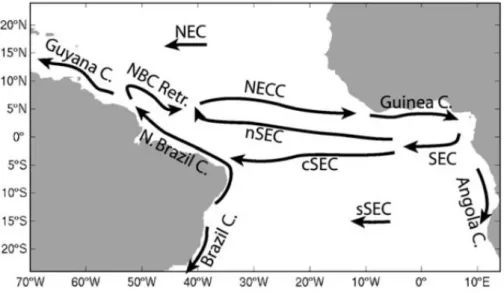
Figure 1.2 shows a schematic of the Tropical Atlantic surface circulation which is bounded by the northern and southern hemisphere subtropical gyres and forms a clockwise equatorial gyre. At the eastern boundary the South Equatorial Current (SEC) is excited and separated at around 5^◦W into a northern and central branch. The central branch of the SEC bifurcates at the western boundary into the North Brazil Current (NBC) to the north and into the Brazil Current to the south. The NBC is the western boundary current of the equatorial gyre. It flows northward, crosses the equator and partly retroflects eastward into the EUC (e.g. Lumpkin and Garzoli [2005]) while the remaining NBC flows further north until it retroflects at 7^◦N into the eastward flowing North Equatorial Counter Current (NECC). At the retroflection point eddies are generated which propagate north-westward along the coast and contribute to the interhemispheric exchange of mass and heat associated with the upper limb of the AMOC (Garzoli et al. [2003]).

At around 5^◦-7^◦N the North Equatorial Counter Current (NECC) flows eastward and hits the African coast, from where it is called the Guinea Current which flows along the coast and eventually closes the equatorial gyre. The NECC is strongest during boreal summer (Peterson and Stramma [1991]) driven by the large-scale seasonality of the trade winds and the seasonal shift of the Intertropical Convergence Zone (ITCZ) (Stramma and Schott [1999]). The southernmost location of the ITCZ in boreal spring leads to a weakening or even reversed westward flow of the NECC (Schott et al. [1998]). Between the NECC and the northern branch of the SEC another strong horizontal shear region is found. Together with the shear between the nSEC and EUC (Jochum and Murtugudde [2004]) these two regions are believed to be responsible for the generation of Tropical Instability Waves (TIWs) due to the meridional shear of the zonal currents which produces barotropic instabilities (von Schuckmann et al. [2008]). In the southern hemisphere TIWs are forced exclusively by baroclinic instabilities while for the northern hemisphere von Schuckmann et al. [2008] showed that both barotropic instabilities due to the horizontal shears between nSEC/NECC and nSEC/EUC and baroclinic instability due to the vertical shear of the nSEC contribute to the generation of TIWs. Calculations of seasonal changes of the instability production rate of the nSEC/NECC shear showed relatively high values suggesting that the strong seasonality of the NECC dominates the seasonal cycle of the TIWs at this latitude.

At intermediate depth Figure 1.1 reveals a meridional alternation of zonal currents. Below the EUC the westward flowing Equatorial Intermediate Current (EIC) is observed with

(13)

1 Introduction

two surrounding eastward flowing cores at around 2^◦ off the equator: the Northern and Southern Intermediate Counter Current (NICC and SICC) with mean zonal velocities of 10-15 ^cm_s (e.g. Schott [2003], Brandt et al. [2006]) which are also called extra-equatorial jets (Gouriou et al. [2001], M´enesguen et al. [2009]). The Equatorial Intermediate Cur- rent System (EICS) is believed to be similarly generated as the EDJs. As for the EDJs D’Orgeville et al.[2007] andHua et al.[2008] suggested instabilites of intraseasonal Yanai Waves as a generation mechanism.

Figure 1.2: Schematic of the mean surface currents in the Tropical Atlantic Ocean based on drifter observations. The abbreviations are explained in the text. Taken from Lumpkin and Garzoli [2005].

The mean cross-equatorial structure of meridional velocities is dominated by shallow near-surface overturning cells in the upper 100m, the so called tropical cells (TC), located between 5^◦N and 5^◦S (e.g. Perez et al. [2013]). They are generated by wind-driven equatorial upwelling, poleward wind-driven flow at the surface, off-equatorial downwelling at 3-5^◦ N/S and equatorward geostrophic flow at the subsurface in about 100m depth. The tropical cells are disturbed by the seasonal appearance of the Atlantic cold tongue and associated Tropical Instability Waves close to the surface which are most pronounced in boreal summer due to intensified south-easterly trade winds and increased shear between the equatorial zonal currents.

(14)

1 Introduction

1.2 Tropical Instability Waves

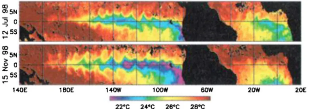
Tropical Instability Waves (TIWs) are common to both the Equatorial Atlantic and Pacific Ocean (Chelton et al.[2000]). They are often described as undulations of the seasonal sea- surface temperature (SST) between 5^◦N-5^◦S but are visible in sea surface height anomalies and meridional velocities as well. Figure 1.3 shows the characteristic SST structure of TIWs for two different time periods in 1998 from satellite measurements. The TIWs appear as near-surface waves with periods of 20-60 days, zonal wavelengths of 400-1500km, westward phase speeds of 20-60 ^cm_s and a stronger signature in the northern hemisphere (e.g. Steger and Carton [1991],Qiao and Weisberg [1995]).

Athie and Marin [2008] noted that there are two different sources of Tropical Instability Waves. The first one results from barotropic instabilities (e.g. Philander [1978]) arising from the horizontal velocity shear of seasonally varying zonal currents: at the surface between the nSEC and NECC or within the thermocline layer between the nSEC and EUC (see Figure 1.1). Barotropic instabilities obtain their energy from the mean background flow (kinetic energy). The second source is baroclinic instability, e.g. due to the equatorial upwelling front, the vertical shear of the northern South Equatorial Current (nSEC) (von Schuckmann et al. [2008]) or the meridionally shoaling thermocline (e.g. Yu et al. [1995]). Baroclinic instability requires the presence of horizontal density gradients causing horizontal variability of geostrophic flow with depth. In contrast to barotropic instabilities, baroclinic instabilities obtain their energy from the stratified water column (potential energy). It is believed that both types of instability contribute to the generation of TIWs in the Atlantic Ocean (Jochum et al. [2004], Grodsky et al. [2005]).

Figure 1.3: 3-day composite-average maps of SST from satellite measurements for 11-13 July 1998 (top) and 14-16 November 1998 (bottom). Black represents land or rain contamination. Taken from Chelton et al. [2000].

The propagation of Tropical Instability Waves can be explained either as westward propagating Rossby Waves along 5^◦N with periods greater than 30 days (Jochum and Malanotte- Rizzoli [2003]) or as mixed Rossby-Gravity Waves (hereafter called Yanai Waves) close to

(15)

1 Introduction

the equator with periods within the intraseasonal time scale between 15-40 days (D¨uing et al. [1975], Weisberg et al. [1979]). As mentioned above TIWs have a larger amplitude in the northern hemisphere but also occur in the southern hemisphere (Steger and Carton [1991]). Bunge et al. [2007] suggested different forcing mechanisms for northern and southern hemispheric TIWs since they could not find clear relations between the two signatures in SST. The interannual variability of TIW activity is significant (Steger and Carton [1991]) and often related to changes of the intensity of the Equatorial Atlantic cold tongue. More precisely, the period and position of TIWs depend on the timing of the seasonal equatorial cold tongue while larger wavelengths and faster phase speeds are associated with stronger equatorial upwelling (Athie and Marin [2008])

TIWs have a significant impact on the mixed layer heat budget due to two processes:

advective and diapycnal heat fluxes. During summer, when the equatorial cold tongue is most pronounced, horizontal temperature gradients develop. Tropical Instability Waves disturb this sea-surface temperature front by advecting warm water into regions of cold water and vice versa. When the water parcels return to their initial position a net heat flux has occured. This heat flux is mainly executed meridionally (1^◦-2^◦C per month) and less zonally (0.5^◦-1^◦C per month) into the cold tongue (Jochum et al. [2007]). Addition- ally microstructure measurements indicate the impact of TIWs on the diapycnal heat flux. During the presence of a TIW elevated turbulence is observed below the mixed layer leading to diapycnal heat flux from the mixed layer into the deep ocean (Moum et al.

[2009]). Weisberg and Weingartner [1988] estimated the equatorward heat flux of the TIWs in the upper 50m with 100 _m^W2 which is comparable to the atmospheric heat flux.

Since TIWs disturb SST fronts they furthermore have an impact on the momentum flux by projecting their mesoscale cusp-like structure onto the surface wind stress. Winds tend to be stronger over warm water and weaker over cold water (Chelton et al. [2001]) which effects the stratification of the atmospheric boundary laver. A flow from warm to cold SST increases the stratification and consequently decreases near-surface wind stress while the effect reverses for a flow from cold to warm SST. This way TIWs have a strong impact on local atmospheric pressure gradients and changes of the wind stress curl which further influences local weather.

Eventually Tropical Instability Waves are the main source for Yanai Waves at the equator.

Parts of the energy of TIWs is radiated into the deep ocean as intraseasonal Yanai Wave beams which will be discussed in 1.3.1.

1.3 Meridional velocity variability

Observations of equatorial zonal and meridional velocity variability reveal two very different spectra for the two horizontal velocity components (Bunge et al. [2008]). The zonal velocity spectrum is dominated by variability with longer periods in contrast to the

(16)

1 Introduction

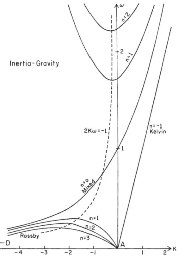
meridional velocity spectrum which shows peaks in the intraseasonal (10-50 days period) frequency range. Philander [1978] noted that this is due to the presence of equatorial waves. Variability on long time scales is associated with equatorial Kelvin and Rossby Waves. Equatorial Kelvin Waves are a completely zonal velocity feature with no associated meridional velocity at all, while equatorial Rossby Waves generate meridional velocities but are limited to lower frequencies. The dispersion diagram for equatorial waves (Figure 1.4) shows that Yanai Waves (called mixed Rossby-Gravity Waves in Figure 1.4) could be an adequate explanation for deep intraseasonal variability in the Tropical Atlantic Ocean.

However numerical studies showed that the presence of the mid-Atlantic ridge close to the equator at 23^◦W could be a source of meridional velocity variability on longer time scales than the distinct intraseasonal signal. McPhaden and Gill [1987] numerically showed that a submarine ridge in the path of a propagating equatorial Kelvin Wave generates meridional motions.

1.3.1 Intraseasonal

Observations and numerical simulations show that the dominant signal of meridional velocity variability in the Equatorial Atlantic Ocean is found on intraseasonal (10-50 days period) time scales (e.g. Ascani et al.[2015]). Close to the surface the intraseasonal signal is associated with monthly Tropical Instability Waves but in the deep ocean other sources must be responsible. The so called deep equatorial intraseasonal variability (DEIV) is believed to be the source of the deep equatorial circulation (DEC) which includes the EDJs and the Equatorial Intermediate Current System (EICS). In general intraseasonal variability arises from two different sources: Tropical Instability Waves (TIWs) with observed periods between 15-50 days and directly wind-forced intraseasonal variability with periods of approximately 15 days (Athie and Marin [2008]).

Realistic numerical simulations showed that a large fraction of the energy that is provided by intraseasonal TIWs radiates into the deep ocean as downward- and eastward- propagating beams of monthly periodic Yanai Waves (von Schuckmann et al. [2008],As- cani et al. [2010]). Figure 1.4 shows the dispersion relation for equatorial waves in the ω-k (frequency - zonal wavenumber) space. Here the unit of frequency is √

βc_m , where β is the coriolis parameter on an equatorial β-plane with f = βy and c_m is the gravity wave speed of the m-th baroclinic vertical mode. The unit of the zonal wavenumber is the inverse of the radius of deformation ^q^c_β^m. The dispersion relation for Yanai Waves is as follows (Gill [1982]):

c_Y =±c_m

s β

k²c_m + β ωk + 1

Yanai Waves are defined by a single meridional mode. The phase velocity (^ω_k) can be either positive or negative which means that Yanai Waves are able to propagate either

(17)

1 Introduction

eastward or westward while their group velocity (^∂ω_∂k) is always positive (eastward). They are antisymmetric about the equator in the zonal velocity component but zero at the equator while being symmetric about the equator in the meridional velocity component.

Eventually there is only a meridional velocity component at the equator due to Yanai Waves. Weisberg et al. [1979] observed a monthly periodic Yanai Wave with upward and westward phase propagation, downward and eastward group propagation and a zonal wavelength of approximately 1200km.

Figure 1.4: Dispersion relation (ω-k) for waves on an equatorialβ-plane forω >

0. The dashed line connects the extrema and n represents the meridional mode.

Taken from Cane and Sarachik[1976].

Yanai Wave dynamics and interaction are a crucial part of the forcing mechanism of Atlantic EDJs and the Atlantic EICS. D’Orgeville et al. [2007] and Hua et al. [2008]

numerically showed that EDJs and EICS result from the instability of an intraseasonal Yanai Wave, that was generated at the western boundary due to an oscillatory western boundary current. The wave became unstable when reaching a zonal wavelength of about 3^◦ and forced both small-vertical-scale (EDJs) and large-vertical-scale (EICS) motions.

Ascani et al. [2015] identified two different types of instability. First the self-interaction of Yanai Waves excites EIC-like currents within the wave beam. Secondly Yanai Waves

(18)

1 Introduction

lose parts of their energy mainly to small-vertical-scale waves (higher baroclinic order).

Ascani et al. [2015] further showed that high-frequent waves (like Yanai Waves) with high vertical wavenumber arise as part of the interaction, while low vertical wavenumber signals correspond to Tropical Instability Waves (TIWs) which are generated by instabilities of surface equatorial currents. Instability and nonlinear modication of Yanai Waves is consistent with the maintenance of the Deep Equatorial Circulation (DEC). Ascani et al.

[2010] noted that intraseasonal Yanai Waves are able to modify the potential vorticity of a water parcel when they are breaking due to large amplitudes, further allowing the parcel to have a persistent equatorward drift across potential vorticity contours.

1.4 Zonal velocity variability

Zonal velocity variability can be separated into three dominant periods: semi-annual, annual and interannual. Each of the dominant signals is associated with a vertical baroclinic mode, in which the energy is mostly contained. The second baroclinic mode is associated with the semi-annual cycle, the fourth baroclinic mode is associated with the annual cycle and the 17th baroclinic mode is associated with the interannual Equatorial Deep Jet period of approximately 4.5 years (Claus et al. [2016]). It is often noted that the EDJs are similar to the gravest equatorial basin mode (e.g. D’Orgeville et al.[2007]) but in fact all three dominant signals are located on the resonance line of the gravest equatorial basin mode which basically consists of an equatorial eastward traveling Kelvin Wave, that is reflected at the eastern boundary into a gravest meridional long Rossby Wave but now propagating at a third of the speed of the Kelvin Wave (Cane and Moore [1981]). These three periods can be divided into externally driven (annual and semi-annual) and inter- nally forced (interannual Equatorial Deep Jets). Nevertheless there is also some variability in the zonal velocity component on intraseasonal time scales.

1.4.1 Intraseasonal

Observations show that intraseasonal variability can also be dominated by zonal velocity fluctuations (Brandt et al. [2006]) but there is a strong year-to-year variability of these intraseasonal fluctuations which is possibly due to the interannual variability of the equatorial zonal current system. These intraseasonal fluctuations are either westward propagating and associated with TIWs (Weisberg and Weingartner [1988]) and vortices (Foltz et al.[2004]) or eastward propagating and coming from the western boundary with periods between 35-60 days (Brandt et al. [2006]).

Below the near-surface layer fluctuations in the zonal velocity component with shorter periods than the cut-off-period of equatorial Rossby Waves (approximately 32 days for the first meridional and first baroclinic mode) are reducing and meridional velocity vari-

(19)

1 Introduction

ability dominates (often called the Deep Equatorial Intraseasonal Variability (DEIV) (e.g.

Ascani et al. [2015])).

1.4.2 Seasonal

The seasonal cycle of equatorial zonal velocity is dominated by an annual cycle and less contributions of a semi-annual cycle. This annual cycle is the dominant zonal velocity variability. (Brandt et al. [2006]) showed that an annual harmonic can explain more than 50% of the total variance in some parts of their time series. They also noted that the vertical migration of the EUC core is responsible for maximum eastward flow in April (October) above (below) the mean EUC core. The seasonal upward and downward motion of the EUC is thought to be forced by variations of the wind stress which itself is forced by the seasonal migration of the Intertropical Convergence Zone (e.g. Provost et al.

[2004], Johns et al.[2014]). Brandt and Eden [2005] gave evidence that the annual signal below the near-surface layer is dominated by downward propagating lowest odd meridional mode Rossby Waves (dominated by the third and higher baroclinic mode). This causes upward phase propagation which implies downward energy propagation. Their principal oscillation pattern (POP) analysis shows a dominant POP that explains about 70 % of the zonal velocity variability and is clearly connected to the annual cycle. The Rossby Waves are either directly driven by zonal wind anomalies or by wind-driven equatorial Kelvin Waves which have been reflected at the eastern boundary (Brandt and Eden [2005]).

1.4.3 Interannual (Equatorial Deep Jets)

On interannual time scales the Equatorial Deep Jets (EDJs) are the dominant signal of variability in the Equatorial Atlantic Ocean. The EDJs are observed in all equatorial oceans. In the 1970sLuyten and Swallow [1976] described them first in the Indian Ocean followed by Hayes and Milburn [1980] in the Pacific Ocean and lastly by Eriksen [1982]

in the Atlantic Ocean. In general EDJs are equatorially trapped zonal velocity features which are geostrophically balanced and alternating in direction with depth and time (e.g.

Johnson and Zhang [2003]). The meridional structure of the EDJs is about 50% wider than expected when considering linear theory based on their observed vertical scale (John- son and Zhang [2003]). Greatbatch et al. [2012] showed with their shallow-water model that this discrepancy can be explained by mixing of momentum along isopycnals. Obser- vations of the Atlantic Ocean EDJs, on which we will focus here, show a characteristic vertical scale of 300-700m, an almost basin wide zonal scale, amplitudes of the order of 10-20 ^cm_s and a period of approximately 4.5 years (Johnson and Zhang [2003],Bunge et al.

[2008]). They are found within a narrow equatorial band of less than 3^◦ latitudinal extent and in depths between the Equatorial Undercurrent at the thermocline (^∼200m) and approximately 3000m (e.g. Bourl`es [2003],Claus et al. [2014]). The eastward jets supply

(20)

1 Introduction

the oxygen minimum zone in the deep eastern Atlantic Ocean with dissolved oxygen from the western boundary (e.g. Brandt et al. [2008]). In the Atlantic Ocean moored velocity data (e.g. Bunge et al.[2008],Brandt et al.[2011],Brandt et al.[2012],Claus et al.[2014], Claus et al. [2016]) and hydrographic data analysis (Johnson and Zhang [2003]) revealed a downward phase propagation of the deep jets which implies upward energy propagation according to linear theory suggesting an influence of the EDJs on near-surface dynamics and properties.

Brandt et al. [2011] showed that the periodic EDJs have a significant impact on SST, wind and rainfall in the tropical Atlantic region. They give evidence that EDJs are linked to changes of equatorial zonal currents of about 6 ^cm_s and changes of eastern Atlantic temperature anomalies of about 0.4^◦C which furthermore can be associated with distinct wind and rainfall patterns. The EDJs propagate energy towards the surface and consti- tute a 4.5-year cycle of SST, wind and rainfall anomalies in the Tropical Atlantic.

The interannual oscillation of the Atlantic Ocean EDJs is unique compared to the other equatorial ocean basins. In the Pacific Ocean they are known to vary on multidecadal time scales (Johnson [2002]) while no dominant signal has been observed in the Indian Ocean. It has to be noted that observational data of EDJs is too short to derive possible multidecadal variabilities for the Atlantic Ocean. EDJs are often associated with the gravest equatorial basin mode (Cane and Moore [1981], D’Orgeville et al. [2007]) which consists of an equatorial eastward traveling Kelvin Wave which is reflected at the eastern boundary into a gravest meridional mode long Rossby Wave propagating at a third of the speed of the Kelvin Wave.

Vertical mode decomposition showed that the energy associated with the EDJs is dis- tributed between the 10th and the 20th vertical mode with a distinct peak at mode 15 (Brandt et al. [2008]) while a more recent study by Claus et al.[2016] suggested the vertical baroclinic modes 16 and 17 following the resonance period of the gravest equatorial basin mode close to the 16th and 17th mode.

To date numerical simulations of the EDJs mainly focused on the generation mechanism of the jets but so far models fail to fully reproduce all characteristics of the EDJs. There is a high dependence on the horizontal and vertical resolution of the model which is why eddy-resolving Ocean General Circulation Models (OGCMs) only inconsistently reproduce the jets. For the Atlantic (Eden and Dengler [2008]) and Pacific Ocean (Ishida et al.

[1998]) it was possible to reproduce the jets when a deep cross-equatorial current at the western boundary is included. In both simulations instabilities of a deep western boundary current led to horizonzal energy propagation into the ocean basin due to Kelvin Wave dynamics but both studies failed to reproduce the vertical propagation and low-frequency basin modes. More recent simulations with sufficient horizontal resolution are able to reproduce the EICS but not realistic depths for the extent.

In general there are two proposed forcing mechanisms for the EDJs. First D’Orgeville

(21)

1 Introduction

et al. [2007] and Hua et al. [2008] showed that large vertical scale, zonally short Yanai Waves propagate westward and are destabilized by barotropic shear instabilites of the equatorial zonal currents forming zonal jets with small vertical scale. It showed that the zonal scale of the Yanai Waves governs the vertical scale of the jets. SecondAscani et al.

[2015] recently showed that intraseasonal Yanai Waves - which are generated by barotropic and baroclinic instabilities close to the surface - interact non-linearly via the meridional advection term (v^∂u_∂y) of the zonal momentum equation. The rectification of the DEIV forms small vertical scale jets (EDJs) and large vertical scale currents (EICS) comparable to the observations. Furthermore the EDJs are found to contribute to the maintenance of the EICS which implies a nonlinear energy transfer that is more complex than thought.

Nevertheless the approach of Ascani et al.[2015] could not explain the vertical scale and the direction of vertical propagation.

However the energy source of the Equatorial Deep Jets is still under debate and is further investigated in this work on the basis of observational moored velocity data.

(22)

2 Data and Methods

2.1 Data

Within the framework of this thesis a variety of moored velocity data from 9 mooring periods and almost 14 consecutive years has been assembled (see Figures 2.1 and 2.2).

Since 2001 the equatorial 23°W mooring has been maintained and exchanged on a regular basis (except for one period between December 2002 and February 2004, where no mooring was mounted). Table 2.1 shows a list of all equatorial moorings that were used in this work together with the deployment/recovery date and the recovering research cruise. The main purpose of the equatorial 23°W mooring is the detection, measurement and analysis of the equatorial current system both in time and space which is why it is mostly composed of mechanical and acoustical velocity measuring instruments.

Time Period Mooring Cruise (Recovery) 14.12.2001 - 21.12.2002 PM-271-A RV Le Suroit (PIRATA-FR11) 13.02.2004 - 29.05.2005 PM-425-A RV Le Suroit (PIRATA-FR13) 30.05.2005 - 19.06.2006 PM-514-A RV Meteor 68/2

20.06.2006 - 01.03.2008 KPO-1001 RV L’Atalante (GEOMAR4) 02.03.2008 - 05.11.2009 KPO-1023 RV Meteor 80/1 06.11.2009 - 02.06.2011 KPO-1044 RV Maria S. Merian 18/2 03.06.2011 - 06.11.2012 KPO-1063 RV Maria S. Merian 22 07.11.2012 - 03.05.2014 KPO-1089 RV Meteor 106 04.05.2014 - 21.09.2015 KPO-1125 RV Meteor 119

Table 2.1: Overview of equatorial moorings at 23^◦W. The first three mooring periods were deployed within the PIRATA program. Since 2006 the physical oceanography department of GEOMAR Helmholtz Centre for Ocean Research in Kiel operates this mooring.

There are two very promising aspects about the equatorial 23^◦W mooring. First the setting of the mooring changed only slightly in the course of time producing long time series for a large depth range and now covering more than two and a half EDJ cycles. But deploying instruments does not always lead to recovering data; especially in the case of the moored profiler (see section 2.1.3). So secondly it should be noted that the fraction of successfully recovered velocity data - especially upper ocean measurements - is remarkable.

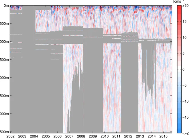
In fact consecutive ADCP measurements are available for a period from early 2004 until late 2015 and a depth range of at least 300m - still continuing. All available velocity data

(23)

2 Data and Methods

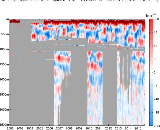
(from moorings and CTD/lADCP) was collected and then combined on a grid that is uniformly distanced both in space and time (see section 2.2.2 and Figures 2.1 and 2.2).

2002 2003 2004 2005 2006 2007 2008 2009 2010 2011 2012 2013 2014 2015 0m

500m

1000m

1500m

2000m

2500m

3000m

3500m

[cms⁻¹]

<−20

−15

−10

−5 0 5 10 15

>20

Figure 2.1: Interpolated zonal velocity (14.12.2001 - 21.09.2015) at 23°W/Equator. Vertical resolution: 1m; temporal resolution: 12h. Higher velocities than 20 ^cm_s are darkred to account for large velocities within the EUC.

Grey areas represent missing data. Single point measurements are expanded to 10m width around true depth.

2.1.1 ADCP

Acoustic Doppler Current Profilers (ADCP) are a very useful measuring instrument to collect velocity data in the upper ocean. They make use of the Doppler Effect which describes a frequency shift (∆f) of an acoustic signal (emitted frequencyf0) when colliding with and reflected by a moving object (traveling speed ∆v - relative to the emitter):

∆f = ∆v c f₀

The ADCP periodically emits an acoustic signal with known frequency. The signal is reflected at biological particles which are purely moved by the underlying ocean velocity.

(24)

2 Data and Methods

The frequency shift of the reflected signal is received from the ADCP and with the according speed of sound profile (c) it can be processed into horizontal velocity data. ADCPs are either deployed in moorings, attached to research vessels (vessel mounted (vmADCP)) or attached to CTD rosettes (lowered ADCP).

2002 2003 2004 2005 2006 2007 2008 2009 2010 2011 2012 2013 2014 2015 0m

500m

1000m

1500m

2000m

2500m

3000m

3500m

[cms⁻¹]

<−20

−15

−10

−5 0 5 10 15

>20

Figure 2.2: Interpolated meridional velocity (14.12.2001 - 21.09.2015) at 23°W/Equator. Vertical resolution: 1m; temporal resolution: 12h. Grey areas represent missing data. Single point measurements are expanded to 10m width around true depth.

The upper 600-800m of the mooring are well covered by ADCPs. Since 2008 upper ocean velocity data is merged from two opposingly orientated ADCPs at approximately 200m depth just below the Equatorial Undercurrent. The upward-looking ADCP covers the subsurface velocity field while the downward-looking ADCP reaches depths of up to 900m during the later mooring periods (see Figure 2.1). Prior to 2008 only one down-looking ADCP was deployed close to the surface and therefore not reaching the same depths as in the later mooring periods. From December 2001 until December 2002 an ADCP was deployed as part of the Prediction and Research Moored Array in the Atlantic (PIRATA).

Although it only reaches about 100m depth it is included in this data set for the reason that this mooring has already been used in studies likeBunge et al.[2007] and furthermore

(25)

2 Data and Methods

delivers single point velocity measurements between 200-1500m.

2.1.2 Single Point Measurements

Where the range of the ADCPs ends single point measurements take over. During the length of the time series different mechanical and acoustical instruments where deployed including Rotor Current Meters (RCM), Argonauts and Aquadopps to measure single depth horizontal velocities. These instruments are a very effective way to fill up the gap between the ADCP and the McLane Moored Profiler (MMP) with additional velocity data at certain depths.

Due to the vertical movement of the instruments - which is a consequence of the occasional tilt of the mooring wire - the depth of the instruments differs from the preset depth and whenever possible velocity data from single point measurements was moved from the preset depth to corrected depths by using other moored instruments which measured pressure. Even though the gap between ADCP and MMP is reducing due to better perfor- mances of the down-looking ADCP single point measurements are another important and independent source of velocity data with a high temporal resolution of 2-hourly values.

2.1.3 McLane Moored Profiler (MMP)

Since 2006 a new method of sampling deep ocean velocities and properties has been used with partial success. The McLane Moored Profiler (MMP) is part of the mooring structure ever since and supposed to record velocity data with an Acoustic Current Meter (ACM) between 1000-3500m (Doherty et al. [1999]). A CTD and occasionally an optode are additionally attached to the instrument to measure salinity, temperature, pressure and oxygen. In contrast to the ADCP the ACM does not make use of the Doppler shift but uses the travel time. While the ADCP relies on backscattering due to particles in the water, the MMP uses an ACM sting with four fingers (emitters) extending at a 45° angle away from a central post (receiver). On two horizontal paths and one vertically angled path a signal is constantly emitted and received by the central post. The emitted signal reaches the central post depending on the underlying ocean velocities. It arrives faster when the current flows in the same direction and vice versa. A speed of sound profile is approximated and later in the processing procedure newly calculated. Additional measurements of the three magnetic compass components and two tilt components are necessary (and performed by the MMP) to convert raw path-coordinated velocity into cartesian-coordinated east, north and vertical velocity.

Every 3-5 days (depending on the programmed setting which is based on the duration of the mooring and the battery life) the MMP is starting from the preset bottom pressure (approximately 3500dbar) and working its way up along the mooring wire with the help of a drive motor while sampling velocities, temperature, salinity and pressure. Immediately

(26)

2 Data and Methods

after reaching the preset top pressure (approximately 1050dbar) the MMP samples another profile on its way down before resting for another 3-5 days. The coverage of almost 2500dbar by only one instrument is very promising but unfortunately it turns out that the MMP is not as reliable as e.g. the ADCP. The moored profiler is very sensitive to biofouling and other sources of resistance on the mooring cable. Figure 2.1 shows that from six deployments only two MMPs yielded complete data sets, two yielded partially complete data sets and another two yielded no data at all (of which one was lost during the mooring recovery and one stopped working right after being deployed). Although these are large gaps in the data set the value of the complete and even partially complete data sets is outstanding. EDJs and intraseasonal variability can now be observed and tracked into the deep ocean.

2.1.4 lADCP

Lastly, whenever available, lowered ADCP (lADCP) profiles have been added to the data set. After each mooring period CTD profiles are performed with an attached ADCP.

Basically between all mooring periods one profile is added which covers the whole water column for one time step (it takes approximately 2-3 hours for a CTD profile of 3500m depth). Just as single point measurements lADCP measurements are a good way of confirming other velocity data and are included for the sake of completeness.

2.1.5 Further mooring data

For further analysis (e.g. the calculation of the Reynolds-Stress described in 2.2.6) moored velocity data from 0.75^◦N (KPO-1002, KPO-1024, KPO-1045) and 0.75^◦S (KPO-1003, KPO-1022, KPO-1043) has been assembled. Zonal and meridional velocities for both moorings are shown in Figures 2.3, 2.4 and Figures 2.5, 2.6. Table 2.2 gives an overview of the moorings, the deployment/recovery date and the recovering research cruise. These two near-equatorial moorings were operated for three consecutive mooring periods between June 2006 and June 2011. For the last mooring period a McLance Moored Profiler has been added to the mooring structures but unfortunately only the MMP south of the equator produced data. With the near-equatorial moorings meridional gradients can be calculated which is necessary for the Reynolds-Stress analysis.

The gridding and interpolation procedures are the same as for the equatorial mooring and will be explained in detail in section 2.2.2.

(27)

2 Data and Methods

Time Period Mooring Cruise (Recovery)

0.75^◦N

20.06.2006 - 29.02.2008 KPO-1002 RV L’Atalante (GEOMAR4) 06.03.2008 - 03.11.2009 KPO-1024 RV Meteor 80/1 03.11.2009 - 04.06.2011 KPO-1045 RV Maria S. Merian 18/2

0.75^◦S

18.06.2006 - 04.03.2008 KPO-1003 RV L’Atalante (GEOMAR4) 04.03.2008 - 06.11.2009 KPO-1022 RV Meteor 80/1 12.11.2009 - 02.06.2011 KPO-1043 RV Maria S. Merian 18/2

Table 2.2: Overview of moorings at 23^◦W / 0.75^◦N/S .

(28)

2 Data and Methods

2007 2008 2009 2010 2011

0m

100m

200m

300m

400m

500m

600m

700m

800m

900m

1000m

<-20 -15 -10 -5 0 5 10 15

>20 [cms^-1]

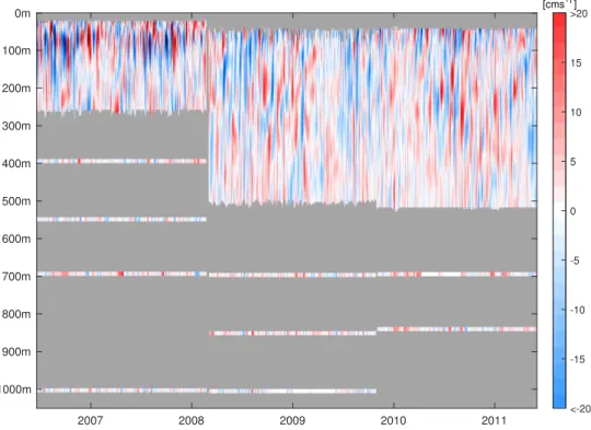
Figure 2.3: Interpolated zonal velocity (20.06.2006 - 04.06.2011) at 0.75^◦N/23^◦W. Red colours indicate eastward flow, blue colours indicate westward flow. Grey areas represent missing measurements. Single point measurement are expanded to 10m width around nominal depth. The resolution is 1m x 12h.

2007 2008 2009 2010 2011

0m

100m

200m

300m

400m

500m

600m

700m

800m

900m

1000m

<-20 -15 -10 -5 0 5 10 15

>20 [cms^-1]

Figure 2.4: Interpolated meridional velocity (20.06.2006 - 04.06.2011) at 0.75^◦N/23^◦W. Red colours indicate eastward flow, blue colours indicate westward flow. Grey areas represent missing measurements. Single point measurement are expanded to 10m width around nominal depth. The resolution is 1m x 12h.

(29)

2 Data and Methods

2007 2008 2009 2010 2011

0m

500m

1000m

1500m

2000m

2500m

3000m

3500m <-20

-15 -10 -5 0 5 10 15

>20 [cms^-1]

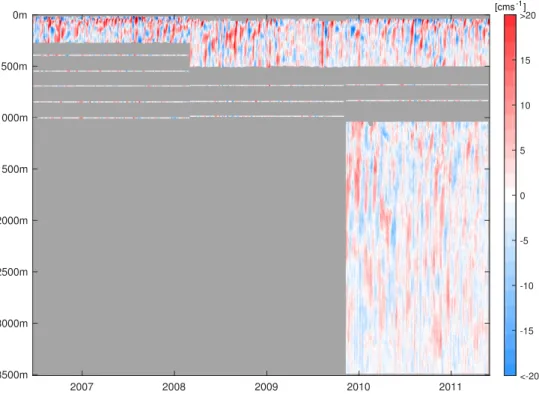
Figure 2.5:Interpolated zonal velocity (18.06.2006 - 02.06.2011) at 0.75^◦S/23^◦W.

Red colours indicate eastward flow, blue colours indicate westward flow. Grey areas represent missing measurements. Single point measurement are expanded to 10m width around nominal depth. The resolution is 1m x 12h.

2007 2008 2009 2010 2011

0m

500m

1000m

1500m

2000m

2500m

3000m

3500m <-20

-15 -10 -5 0 5 10 15

>20 [cms^-1]

Figure 2.6: Interpolated meridional velocity (18.06.2006 - 02.06.2011) at 0.75^◦S/23^◦W. Red colours indicate eastward flow, blue colours indicate westward flow. Grey areas represent missing measurements. Single point measurement are expanded to 10m width around nominal depth. The resolution is 1m x 12h.

(30)

2 Data and Methods

2.2 Methods

2.2.1 Processing of the MMP data

Part of this thesis and prior work was the processing of moored velocity data from the McLane Moored Profiler (MMP) and the equatorial 23^◦W mooring deployments KPO- 1089 (2012-2014) and KPO-1125 (2014-2015). This section only gives an overview of the whole process. For a more detailed description of the processing procedure seeDidwischus [2010].

For each vertical profile three binary files (one each for CTD data, ACM data and engineering data) is written to the flash memory card of the MMP. The CTD-files contain conductivity, temperature and pressure measurements while the ACM-files contain the two tilt components of the instrument, horizontal and vertical magnetic compass components and velocity data from the four pathways described above. The engineering files contain time information, electrical voltage and current, pressure and - if measured - oxygen data. Additionally the engineering files record the starting and end time of the sensors and the drive motor as well as the reason for finishing a profile which is important for future deployments. With an unpacking software the binary files are converted into ”human readable” .TXT-files which are now processed in four major steps: first the merging of the raw data files, second the pressure gridding, third the velocity scaling and lastly the CTD conductivity calibration.

Since there are three .TXT-files for each profile (CTD, ACM and engineering data) the first step of the processing is the merging of these three .TXT-files into one .MAT-file per profile. Secondly as CTD and ACM are measuring with different sampling rates (approximately 4 and 3 Hz) it is necessary to interpolate both data sets onto the same time vector. Under the assumption of a constant sampling rate of the CTD and by including the pressure measurements of both the CTD and the engineering files a time vector is interpolated for CTD data. Consequently a starting and end point is calculated for each profile which is used to interpolate the velocity data within these points to temporally combine all three data sets. Then conductivity, temperature and pressure sensor values are calibrated by using polynomial fits from laboratory calibrations. Lastly the second step contains the compass calibration by determining the compass bias with a previously done laboratory compass spin test. It is difficult to reach precise values for the compass bias with a spin test so we chose another approach by calculating vertical mean velocities of the two horizontal components over the time series of the MMP and rotating both components. Under the assumption that the EDJs only project onto the zonal velocity the vertical mean profile of zonal velocity with the highest standard deviation over depth is chosen to be the one with the best guess of the compass bias. Similarly vertical mean profiles of meridional velocities are assumed to be rather barotropic and have a small standard deviation over depth.

(31)

2 Data and Methods

The third step deals with deriving east, north and vertical velocities from raw ACM velocity path data and correcting them for the horizontal movement of the MMP during the casts. Before the correction high frequent velocity structures within one profile are filtered out. The horizontal movement of the MMP is due to the occasional tilt of the whole mooring which can be calculated from the tilt sensors and the vertical speed of the MMP. In general the corrections are lower than 1 ^cm_s . Furthermore the previously assumed sound speed profile is replaced by a newly calculated profile from the measured properties of the water column. After the velocity corrections the velocity data is smoothed by a low-pass filter.

In the last major step conductivity data is calibrated by using temporally and spatially close shipboard CTD measurements and single peaks have to be corrected manually by either interpolation over time with neighboring profiles or over depth with the same profile. After finishing these processing steps the data can be accessed as a .MAT-file for each vertical profile containing finally processed time, conductivity, salinity, potential temperature, pressure, velocity (zonal, meridional, vertical) and engineering data (e.g. electrical current and voltage).

2.2.2 Gridding and combination to one dataset

Since all moored velocity instruments have different temporal resolutions it is necessary to describe how they have been combined. Single point measurements generally sample horizontal velocities every two hours while moored ADCPs have a sample rate of one hour but are already merged in the processing procedure into 12-hour values. The sample rate of the MMP differs over time (depending on the mooring period) between 3 to 5 days per pair of vertical profiles. All data is low-pass filtered with a 40 hour Hamming window to account for high-frequent tidal velocities except for the MMP data, whose low sample rate makes this step unnecessary.

For the combined data set we decided on a temporal resolution of 12 hours and a vertical resolution of 1m. The single point measurements have a preset nominal depth but expe- rience vertical movements due to the occasional tilt of the mooring which easily exceeds 1m. So, whenever possible, pressure data of other moored instruments has been used to quantify this movement and to apply a modified pressure time series to the single point measurements with varying depths for the mooring period. ADCP velocity data is usu- ally binned into 5 or 10m values which made vertical interpolation necessary in order to achieve the aimed vertical resolution. Since CTD and ACM of the MMP have sample rates well beyond 1 Hz - while moving up and down the wire with about 45 ^cm_s - velocity data has already been processed on a 1m grid.

In the temporal direction single point measurements were interpolated into 12-hour values and combined in space with ADCP data. Especially in the case of KPO-1089 and KPO-

(32)

2 Data and Methods

1125 ADCP measurements reached down to depths where single point measurements were installed and supposed to measure horizontal velocities. If depths were double covered both time series were compared and always found to basically be identical. The inclusion of MMP data was more complicated. The time vector is defined by the ADCP and single point measurements. First of all for time steps where MMP velocities were measured the data was included into the 12-hourly resolved grid and the time steps between two pairing vertical profiles of MMP velocity had to be filled with empty data (NaNs). These gaps were as large as 5 days depending on the mooring. This way up- and downward profiles were placed next to each other followed by NaNs. Then whenever possible the gaps were filled by interpolation over time between values at the same depth to guarantee continuous data within the depth range of the profilers. The largest interpolated gaps were 7 days long while all larger gaps were ignored and chosen to be filled with NaNs.

All interpolation steps in the vertical and the temporal direction were compared to unin- terpolated data and found to be realistic. If not further noticed the following analysis steps are based on the interpolated data sets shown in Figure 2.1 and Figure 2.2. However for some calculations the data set has been subsampled in order to reduce the computational costs.

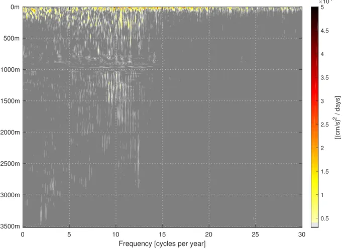
2.2.3 Spectral Analysis

Because of the gaps in the velocity data set it was not possible to calculate the frequency spectrum of the horizontal velocity components with a common Fourier-Transformation.

Instead a Lomb-Scargle periodogram has been calculated for the reason that the time series does not have to be uniformly spaced, thus allowing data gaps (Scargle [1982]).

Unfortunately this way the spectral characteristic of depths with low data coverage is biased and has to be analysed with care. The periodogram (power spectral density (PSD)) for a given frequency ω is estimated by:

P SD(ω) = 1 2

[^P_iX_icosω(t_i−τ)]²

P

icos²ω(t_i−τ) +[^P_iX_isinω(t_i−τ)]²

P

isin²ω(t_i−τ)

!

where X is the analysed time series of zonal/meridional velocity at the time step i, t is the time at time step i and τ the time delay at which the sinusoids would be mutually orthogonal, defined by:

tan(2ωτ) =

P

isin(2ωt_i)

P

icos(2ωt_i)

With this method a Lomb-Scargle periodogram could be calculated for each depth of the zonal and meridional velocity data set with a given frequency vector that is the same as a Discrete Fourier-Transformation (DFT) would produce for a complete time series. The results are shown and described in section 3.1.

(33)

2 Data and Methods

2.2.4 Intraseasonal variability

Intraseasonal variability is quantified by several methods in this work. Spectral analysis has been performed in the way described in the previous section 2.2.3 since it is the same data set with the same gaps. If not otherwise mentioned all low-pass filtering performed in this analysis has been done by applying a Hamming window which is defined as follows:

ω(n) =α−βcos( 2πn N −1)

with α = 0.54 and β = 1− α = 0.46. N represents the width in terms of time steps (hereafter window size) and n is a vector with size N-1.

Interpolated meridional velocities are used to construct a time series of Tropical Instability Waves activity by averaging the upper 50m and then deriving the kinetic energy v² at each time step. From the time series it was possible to construct a climatological cycle on the basis of almost 14 years of data (with two gaps between December 2002 - May 2005 and June 2006 - March 2008). The high resolution of two values per day makes low-pass filtering necessary in order to visualize seasonal signals in the time series. The filtering was performed as described above.

Finally harmonic cycles are fitted to the data to emphasize the annual and semi-annual signals within the climatology. The harmonic cycles are constructed by searching for the amplitude a₁ and the phase a₂ of the model function

x=a₁cos(2π

T (t−a₂))

which minimize the covariance between the difference of this function and the original time series. A preset time vector t and a period T (e.g. 365 days for the annual harmonic cycle) have to be provided.

The characteristics of chosen Yanai Wave beams that will be analysed in this work are extracted as follows. The phase speed of a Yanai Wave is upward propagating. Within a certain time and depth window maxima (or minima) of meridional velocity are identified.

Then a linear fitting model is chosen to approximate the phase propagation in a least- square sense. The resulting slope of the fit is the phase speed while the vertical distance between the phases will be the approximation of the vertical wavelength of a single beam.

2.2.5 Vertical Mode Analysis

For the vertical mode analysis the vertical mean profiles of zonal and meridional velocities have been calculated (see Figure 3.10) and subtracted from the data. Then subsampling in both time and space was necessary to keep the computational cost on a minimum while simultaneously including as much information as possible. In the end we decided on daily

(34)

2 Data and Methods values and 10m spacing in the vertical for further analysis.

With a fitting model similar to the oneClaus et al.[2016] used it is possible to decompose the horizontal velocity components into normal modes:

u(z, t) = ˆp_n(z)a_nωe^iωt+a^∗_nωe^−iωt

For a set of frequencies f (with ω = 2πf) and a chosen range of vertical baroclinic normal modes n (for n=1,2,...,20) observational zonal and meridional velocities are fitted to vertically propagating linear waves. For each depth (z), time step (t), frequency (f) and vertical normal mode (n) complex fitting coefficients anω and a^∗_nω were calculated and combined with the vertical mode structure function ˆp_n(z). The baroclinic vertical modes are derived from a mean equatorial stratification profile at the mooring position at 23^◦W and normalised as follows:

Z 0

−Hpˆ²_ndz = 1

Additionally the barotropic mode ˆp₀(z) is included in the vertical structure function and normalised analogously:

Z 0

−Hpˆ²₀dz = 1

Since the definition of the barotropic mode is its constant velocity with depth the equation simplifies to:

ˆ p²₀

Z 0

−H1dz = 1 ˆ

p₀ =

s1 H

which becomes 1.68 m⁻¹² with a realistic observational depth of H=3539m. Figure 2.7 shows the vertical structure of four different vertical modes. The projected velocities

˜

u are calculated by a normalised scalar product between the original velocities and the structure function in the form of:

˜

u= < u,p >ˆ

||ˆp||

The unit of the projected velocity is then independent of the normalisation of the structure function.

The fitting model u(z,t) is applied onto the original velocity data X(z,t) for each frequency and each vertical mode. First both the model and the data set are reshaped into one- dimensional vectors and the missing values in the velocity data are identified and not considered in the fitting process. The fitting itself is performed by a matrix division:

A=X(z, t)/u(z, t)