Velocity Map Imaging

(1)

Velocity Map

Imaging

(2)

A. Wituschek (8/2016)

Velocity Map Imaging

Institut f¨ ur Mathematik und Physik

(3)

(4)

1 Introduction

The inner structure of matter has been under investigation by mankind over thousands of years. A microscopic structure of matter was postulated by Demokrit around 400 B.C. Since then the theories about the structure have become more and more detailed and revealed a keen knowledge of matter.

In 1814 Fraunhofer discovered dark lines in continuous spectra of sunlight. This was the first hint at a completely new physical theory, a completely new world view. It took some time and the help of Einsteins quantized theory (1905) and Bohrs new atom model (1913) to understand Fraunhofers observation.

Investigating spectra of different systems started to boom during this times. It was not only possible to identify elements in different probes, it was possible to investigate the inner structure of atoms or molecules and to put the new theories to test.

In 1960 the laser was invented and with its help a lot of new spectroscopy techniques where developed like absorption-, laser induced fluorescence-, Raman-, ionization- or time resolved pump-probe spectroscopy.

Measuring the energy- and spatial distribution of photoelectrons makes it possible to investigate the internal electronic structure of the atoms and molecules. The easiest way is to measure the time of flight of the photoelectrons to a detector that is placed at different positions with respect to the ionizing laser field. However, mechanically moving the detector inside a vacuum apparatus is cumbersome. Besides long measuring times are needed. Furthermore, the energy resolution may be limited by the short flight times of electrons up to the detector.

Velocity map imaging (VMI) is a technique which makes it possible to cover the whole solid angle in one measurement and to measure the energies and emission angles of all photoelectrons at once. For this the photoelectrons are imaged onto a position sensitive detector using an electrostatic lens created by inhomogeneous electrical fields. The detected intensity image can be used to draw conclusions on the electron velocity distribution and hence retrieve information about the energy- and spin states of the particles under investigation.

1.1 Goal of the Experiment

The main goal of this experiment is to investigate the electronic structure of Potassium atoms using an effusive Potassium beam in combination with a VMI spectrometer. Furthermore the properties of an effusive atomic beam as well as the spatial intensity distribution of the laser focal volume can be characterized by imaging photoions instead of electrons.

The setup marks the state of the art in terms of velocity map imaging spectrometers employed in atomic and molecular physics and in physical chemistry. Similarly to the course of action in a real research laboratory, a series of preparatory steps are undertaken prior to performing the main measurement.

These include simulations of the setup, as well as characterization and optimization of the performance.

Also a number of optional tasks are included which allow the students to investigate certain phenomena in more detail.

(7)

2 Fundamentals

2.1 The Laser

In this experiment we use a single mode grating stabilized diode laser which emits at approx. 405nm.

For the basic function of a diode laser you may take a look at [4].

This diode laser emits only one single frequency which is tunable in wavelength with a range of approx.

15GHz. There are basically three ways to manipulate the emitted frequency, and all ways interact with one another:

1. One can tune the frequency of the laser diode by changing the current that feeds the diode 2. It is good to know that a diode laser is very sensitive to light falling onto the diode. Therefore it is

necessary to avoid uncontrolled scattering of light into the diode. On the other hand one can use this effect to stabilize the laser frequency by feeding the laser with the right frequency. Right behind the diode a grating in so called Littrow configuration is mounted into the beam which contributes to the stability of the frequency on the one hand and the tunability of the laser on the other hand.

The grating is mounted in such way that the first order diffraction is reflected back into the laser diode. The grating and the backside of the diode constitute an external resonator. This setup stabilizes the frequency of the diode, and can be used to tune the laser to each frequency within the internal amplifying profile of the diode. The diffraction angle is dependent on the frequency of the incoming light. By tilting the grating relatively to the laser diode one can change the emitted frequency of the diode. This tilting is realized with a piezoelectric element.

3. The third way is to change the temperature of the diode which impacts on the band gap of the semiconductor material and therefore changes the frequency of the emitted light.

A very common way of tuning a diode laser and the way we do it in our setup is the so-called Feed Forward procedure. By simultaneously tilting the grating and changing the laser current it is possible to tune the laser in a relatively wide mode hop free range.

Basic information about optics and lasers can be found in [9] or [5].

2.1.1 Optics

Besides mirrors and lenses two optic devices are used to manipulate the laser beam in a non trivial way, aλ/2 plate and a polarizing beam splitter (PBS).

1. λ/2 plate: This plate consists of an anisotropic optical material. This material has different refractive indices for the ordinary and the extraordinary beam. Both beams undergo a phase shift while traveling through the material. One now can chose the length of the material in a way that the relative shift between the two parts of the beam isλ/2. This equals a phase shift ofπ. If now linearly polarized light with an angle of θ to the optical axis of the material passes through the material the polarization afterwards will be −θ. Thus the polarization vector is rotated through an angle of 2θ.

2. The PBS is used to split the beam in two perpendicularly polarized parts. One can write the polarization vector as a superposition of perpendicular and parallel polarization relative to the beam propagation surface. The parallel polarized part of the beam passes through the PBS. The perpendicular polarized part is deflected at right angles. One can use this to check the polarization of the beam behind the λ/2 plate.

(8)

Figure 1: Setup of a polarizing beam splitter [5].

2.1.2 Gaussian Beams

Gaussian beams are a model to describe the propagation of (laser)beams. They combine wave-optics with geometrical-optics. Transversal to the axis of the beam the beam has a Gaussian profile with a minimum of width in the focus of the beam. In direction of propagation the beam has a Lorenz-profile.

In cylindrical coordinates with the origin in the focus of the beam wherezis the direction of propagation andrthe distance from thez-axis one can use following equations to describe the beam:

w(z) =w₀ r

1 + ( z

z_R)² (1)

where w(z) is the width of the laser spot in the plane perpendicular to the propagation. The width of the beam is described by the radius (if the beam is circular) of the beam at 1/e amplitude or 1/e² intensity respectively.

In our setup lenses are used to focus the beam. Under the assumption of a parallel beam falling onto the lens one can calculate the width of the beam in the focus viaw0= 2_πw(z^λf

lens) whereλis the wavelength, w(z_lens) the diameter of the beam before focusing it andf the focal length of the lens used to focus the beam. The zR = ^πw_λ²⁰ is called Rayleigh length. The interval [−zR, zR] is called focal area of the laser.

The laser intensity on the axis of the beam (r= 0) decreases fromI(z= 0) =I₀toI(z=±z_R) = 1/e²I₀.

(9)

2.2 Potassium and its Properties

Potassium is an element in group one (alkali metals) with an atomic number of 19 and term symbol K.

The most abundant isotope is³⁹K(natural abundance 93.26%). All alkali metals are very reactive. This requires a careful handling of elementary potassium. Contact with air humidity results in a dangerous exothermic reaction and the potassium gets useless for this experiment because an oxide shell closes around the elementary potassium. Therefore potassium must be kept under high vacuum conditions or under dry Nitrogen atmosphere. The electron configuration of Potassium is [Ar]4s¹. More detailed information on Potassium can be found in [11].

4s 5s

4p1/2

3d 5p_1/2

5p3/2

0 eV

1.60996 eV

4.34066354 eV

3.0625809 eV 3.0649065 eV 946 nm

∆=0.31 nm / 562 GHz

1.5e+06

1.07e+06 1.16e+06

4.5e+06 A= 4.6e+06

1.4e+06 / 1.5e+05

2.20e+07

1.56e+07 7.9e+06

3.75e+07 3.80e+07 K-level scheme

4p3/2 1.61711 eV 404.52847 nm

404.83565 nm

2.59e+07 / 4.34e+06

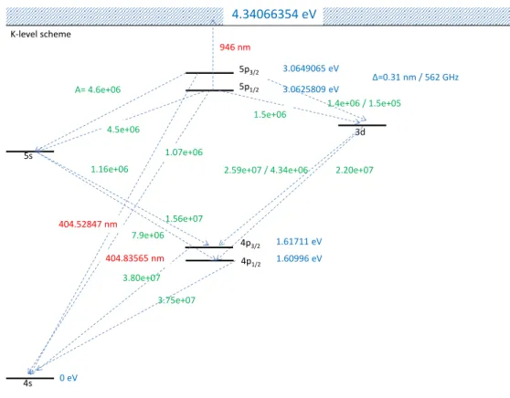
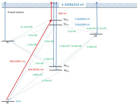
Figure 3: Level scheme of Potassium. In red: wavelengths to excite several states. In green:

Einstein-coefficients for spontaneous decay. In blue: energies of the states

2.3 VMI Spectroscopy

Velocity Map Imaging (VMI) spectroscopy a method to investigate the velocity-distribution of charged particles in a volume. Usually these charged particles are obtained via photoionization. The spatial distribution of the particles is not considered to be under investigation and therefore should not contribute to the results of the measurement.

2.3.1 Setup of the VMI

The VMI spectrometer consists of three parts. The electrodes, the flight tube and the detector system.

The principal setup is shown in figure 4. We use electrodes to create an inhomogeneous field which accelerates the charged particles onto the detector surface. The field must be chosen in such way that the velocity-distribution of the particles is mapped on the detector regardless of the initial spatial distribution. A design of electrodes that satisfies this requirements is theEppink-Parker-Design [6].

(10)

The lowest lying electrode is called repeller followed by the extractor and ground electrodes. All electrodes have a circular layout and are about 1mm thick. The extractor and ground electrodes have a concentric hole. The geometry, distance and applied voltage of the electrodes determine the field that accelerates the charged particles. The ground electrode is necessary to ensure a field free drift region between the electrodes and the detector surface.

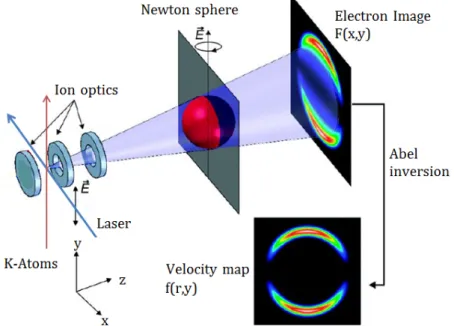
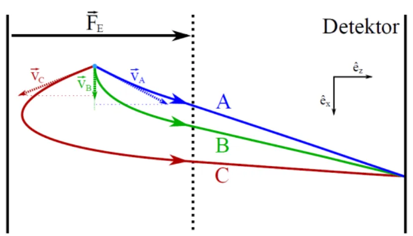
Figure 4: Setup of a VMI Spectrometer: A laser ionizes atoms located between the electrodes.

The electrodes accelerate the charged particles towards a detector. On their way they expand on a Newton sphere because of their kinetic energy. This spherical distribution is projected onto the 2D position sensitive detector surface. The initial velocity distribution can be obtained via a so called Abel-inversion, see section 2.3.2.

The detector consists of three parts:

1. The microchannel plate (MCP) is made of a highly resistive material. Small channels with a diameter of 8µm and a distance of 10µm go through the material. They are tilted relatively to the surface of the MCP. Charged particles hit the front of the MCP where they generate electrons. A high voltage (max. 1kV) is applied between the MCP front and the MCP back. This accelerates the electrons forward to the MCP backside. These electrons hit the wall of the channel and generate new electrons. In this way an avalanche of electrons exits the channel at the back of the MCP.

The typical amplification factor of one MCP plate is around 1000.

2. The electrons leaving the MCP back are accelerated towards a phosphor screen which is biased on a high potential (about 4kV). Electrons hitting the detector cause a light flash in a typical wavelength determined by the used phosphor screen. The light flash of the phosphor that we use takes about 4ms to decay.

3. A charge coupled device (CCD) Camera that is sensitive to the emitted light of the phosphor screen captures the picture and transfers it to a PC.

2.3.2 The velocity distribution

For now we assume the charged particles originating at a point source between the repeller and extractor

(11)

Figure 5: Setup of a microchannel plate [7]

towards the detector. As one can easily see in fig. 6 particles with different velocity vectors can be mapped on the same spot on the detector.

In general some information is lost when mapping a 3D-distribution on a 2D surface. But the original 3D-distribution can be retrieved with the help of the following:

Using symmetry: By using a linearly polarized laser for photoionization one can mark one spatial direction. Regarding to this spatial direction the distribution of the velocity vectors is cylindrically symmetrical.

Using calculus as shown hereafter.

In the following case the polarization direction shall be parallel to the detector surface. We obtain a cylindrically symmetric distributionf(r, y) along the y-axis. We will now show the connection off to its projection F onto the detector. The infinitely far away observant may look at the distribution F along theez-direction, see figure 7. He sees the integrated (along thez-axis) signal:

F(x, y) = Z ∞

−∞

f(r, y)dz= 2 Z ∞

0

f(r, y)dz (2)

Withr²=x²+z²one can obtain

dz= r

√

r²−x²dr (3)

Using substitution following expression forF holds:

F(x, y) = 2 Z ∞

|x|

f(r, y)r

√r²−x²dr (4)

This is the so calledAbel-transform. It calculates the observed imageF caused by a distributionf. 2.3.3 Abel Inversion

We have shown how to determineF out of the initial distributionf. The problem in the experiment is that we observe the distributionF and want to calculate the initial distributionf. It can be shown that following equation forf holds [1, pp. 60-61].

f(r, y) =−1 π

Z ∞

|r|

dF(x, y) dx

√ 1

x²−r²dx (5)

(12)

Figure 6: Particles with different velocities vA,vB andvC with |vB| 6=|vA|=|vC| are mapped on the same spot on the detector. Because of different times of flight the vx components of the particles can differ from one another although they hit the same spot on the detector [7].

Figure 7: In this sketch cuts through the distributionsf(r, y) and F(x, y) are plotted for fixed y = y0. The observer has a look on the distribution along the z-axis and hence always sees a signal which consists of the integrated distribution F along the z-axis [7].

(13)

This is the so-calledInverse-Abel-transform. One can easily see there will be problems reconstructing the initial velocity-distribution out of raw experimental data with the help of this equation. In this case the distributionF is not continuously differentiable because of the finite number of pixels of the used CCD- Camera. For this reason the derivative ofF could only be approximated by differential quotients. These quotients could become irrationally big due to possible noise of single pixels. It would be unreasonable trying to obtainf in this direct way.

2.3.4 The BASEX-Method

The BASEX-Method is an numerical approach to solve the integral in 2.3.3. The idea is to have basisfunctions ¯fk in the space of distributionsf. Their projections ¯Fk onto the detector are well known.

The choice of base functions can be made arbitrarily but it is useful if they satisfy following properties:

every function should be easily analytically integrable to perform the Abel-transformation

intensity-distributions obtained by this transformation shall permit imaging of sufficiently small structures

the projections shall be sufficiently smooth on even smaller distances Following base complies to the upper requirements:

f¯_k(r) =e k²

^k²r σ

^2k² exp

−r σ

²

(6) whereσis a parameter determining the position of the maxima and the spread of the functions over r.

To satisfy the upper requiremetsσshould be chosen in the magnitue of the smallest structure that can be resolved with the detector.

The Abel-transformations of ¯fk are given by:

F¯k(x) = 2σρk(x)



1 +

k²

X

1

"

x σ

−2l l

Y

m−1

(k²+ 1−m)(m−1/2) m

#

 (7)

The Abel-transformation is linear hence the ¯Fk provide a basis in the space of projections. Every measured image can be expressed with this basis. Fork→ ∞ one obtains functions ¯Fk whose maxima are placed at greater values ofx. Using a detector with finite diameter one can limitkdependent on the choice ofσand thus obtain an finite basis. If one now expressesFin terms of ¯Fkthe wanted distribution f is obtained by the respective linear combination of the ¯fk.

Of course there are several different approaches to retrieve the inverted image from the experimental data. An overview is presented in [1, pp. 62-64]. In this experiment we use a program called pBasex which basically uses the BASEX idea in combination with polar basis functions [8].

(14)

Figure 8: Some basis functions f¯k (top) for the BASEX-method and the analytic Abel- transformed functions F¯k mapped on the detector (bottom) [7].

(15)

2.4 Theory of Photoionization

Photoionization means ionization of atoms or molecules with the help of interaction with photons respectively electromagnetic waves. Such a wave can be described using a vector potential:

A(~~ r, t) =A₀ˆexph i

~k·~r−ωti

(8) with A0 the amplitude of the wave, ~k the wave vector, ω the angular frequency, t the time and ˆ a normalized polarization vector with ˆ·~k= 0. The direction of~kis the direction of propagation of the wave, the absolute value is k=w/c= 2π/λ. The vector potential Φ(~r, t) that is usually used together with the vector potential to describe electromagnetic fields vanishes because there is no spatial charge distribution. It is:

E(~~ r, t) =−∂

∂t

A(~~ r, t) (9)

B(~~ r, t) =∇ ×A(~~ r, t) (10) Hence it isE~ kˆandB~ ⊥ˆ.

The interaction of such a field with a single electron bound to an atom in a Couloumb potentialV(~r) can be described via modification of the single particle hamiltonianH₀=~p²/2m_e+V(~r). The hamiltonian of the interacting system is given by:

H = 1 2m_e

~ p−e

c

A(~~ r, t)2

+V(~r) (11)

=H₀+H₁ (12)

with

H₁=− e 2mec

~

p ~A+A~~p + e²

2mec²|A|~ ² (13)

This term can by simplfied using the following assumtions:

1. In couloumb gauge it is∇A~ = 0. Therefore the impulse operator and the vector potential commute hp ~~Ai

= 0

2. The amplitdeA0may be sufficiently small to neglect the quadratic terms 3. Using the long wave approximation it is exph

i~k·~ri

= 1 +i~k·~r+. . . ≈1. This means that the wavelength is much bigger in comparison to the dimensions of the system. Even at interaction of UV-light (λ= 200nm) with atoms or simple molecules (r <1nm) this assumption is justified (~k·~r= 2πr/λ≈0.031).

Therefore it is:

H1=− e

m_ecA0ˆexp(−iωt) (14)

This hamiltonian describes a periodic perturbation. With the help of time dependent perturbation theory one can determine the transition probability of a system from an initial state|iito a energetically higher lying final state|fi(i.e. absorption of a photon~ω). This results inFermi’s golden rulefor the transition

(16)

probability:

W_|ii→|fi= 2π

~

| hf|H1|ii |²δ(Ef −Ei−~ω) (15) For an ionization process the final state |fiis a unbound state of the electron. This can be described via a plane wave with wave vector~κ. The energy eigenvalues of an unbound electrons are continuous.

Hence forW 6= 0 the necessary conditionEf−Ei−~ωneither determines the energy of the photon nor the energy of the photoelectron. If~ω≥(E_f−E_i) the condition can be satisfied by the emission of an electron with the particular energy:

E_f(~κ) = ~κ² 2me

=E_i+~ω (16)

Note that the energy of the bound state|iiis negative due to the convention that the ionization threshold marks the origin of the enrgy axis. The mass of the atom relative to the electron is much higher therefore any energy transfer can be neglected.

2.4.1 Directional Distribution of the Photoelectrons

With eq. 16the energy of the photoelectrons is well defined. To characterize the electrons material wave completely it is necessary to determine the direction of the wave vector~κ. The directional distribution depends on the state|iiof which the atom is ionized. This state is a solution of the time independent Schr¨odinger equation of the unperturbed hamiltonianH0|Ψi=Ei|Ψi. In terms of spherical coordinates one gets:

Ψⁱ_nlm(r, θ,Φ) =R_nlⁱ (r)Y_lm(θ,Φ) (17) This state is characterized with the three quantum numbersn, landmand a product of the radial part Rand the spherical harmonicsY_lm. θshall depict the angle towards the polarization direction ˆ. For the directional distribution of photoelectrons coming out of a state|iione gets [1]:

Jnlm(θ,Φ)∝

κ^−1/2X

L

X

M

−i^Le^iδ^L

YLM(θ,Φ) ˜R^κL_nlY˜_lm^LM

2

(18)

with the radial and angular matrix elements respectively:

R˜^κL_nl = Z ∞

0

R^(f)_κL(r)R⁽ⁱ⁾_nl(r)r³ (19)

Y˜_lm^LM = Z π

0

Z 2π 0

Y_LM^∗ (θ,Φ)Y_lm⁽ θ,Φ) sinθcosθdθdΦ (20) The energyEand the quantum numbersLandM of the final state are defined by the wave vectorκof the photoelectron. δL describes the phase shift of theL^th partial wave.

Because ˜Y_lm^LM 6= 0 for a finite transition probability one gets following selection rules for the transition:

∆l=L−l=±1 (21)

∆m=M−m= 0 (22)

(17)

Therefore eq. 18can be simplified to a sum of two terms;

J_nlm(θ,Φ)∝

rl²−m² 4l²−1

R˜^E,l−1_n,l−1Y_l−1,m(θ,Φ) (23)

−e^i(δ^l+1^−δ^l−1⁾ s

(l+ 1)²−m² (2l+ 3)(2l+ 1)

R˜^E,l+1_n,l+1Yl+1,m(θ,Φ)

2

(24) For|m|=l, the transition toL=l−1 is not possible, the corresponding coefficient becomes zero, and a single term of the sum is left. For|m|< l, the resulting angular distribution is created by interference between the two partial waves with L = l ±1. The interference pattern critically depends on the difference between the phase shifts of these waves, and the ratio of their amplitudes, determined by the radial matrix elements.

As an example, the superposition of the final states (L, M) = (0,0) and (2,0), accessible from an initial (l, m) = (1,0) state, is shown in9. Depending on the phase shifts, both constructive and destructive interference can occur along the laser polarization axis.

Figure 9: On the left: constructive interference alongz. On the right: destructive interference along z [1].

2.4.2 The Anisotropy-Parameter

If one has an ensemble of atoms the directions of the orbital angular momenta are oriented arbitrarily.

Defining a spatial direction ˆwith the help of a linearly polarized laser one obtains all possible projections of the orbital angular momentum on this direction. Hence the measured directional distributionJnl(θ,Φ) is given by averaging over all distributionsJ_nlm(θ,Φ).

For the absorption of a linear polarized photon one has [3]:

J_nl(θ) = 1 +βP₂(cosθ) (25)

HereP₂is the second Legendre polynomial given byP₂(x) = 1.5x²−0.5 andβ∈[−1,+2] the so called anisotropy parameter. The restriction on the given interval is due to Jnl being non negative. β = 0 results in a isotropic distribution,β=−1(+2) in a pure sin²θ(cos²θ) distribution respectively.

2.4.3 Multiphoton Ionization

Besides ionizing an atom with one photon also two- or multi-photon processes are possible. Basically one can distinguish between resonant and non resonant photoionization processes.

Using a non resonant process the electron gets ionized out of its ground state directly. All photons involved in this process have to interact in a very small amount of time which makes the process unlikely to happen at small photon densities. One needs very high laser intensities to realize such a process.

Multiphoton processes at smaller laser intensities can be realized using the REMPI process (resonance enhanced multi-photon ionization). This requires a energy state in between ground state and ionization threshold that is resonant to the energy of the photons. At first electrons get excited in this state via a first photon. During the lifetime of this state a second photon can ionize the electrons out of this state.

(18)

This resonance enhances the probability of the whole process significantly. The easiest case (and our case) is if both photons have the same energy and polarization. One can extend eq. 25on two photon processes:

Jnl(θ) = 1 +β2P2(cosθ) +β4P4(cosθ). (26) Now one has two parametersβ2andβ4,P4= 4.375x⁴−3.75 + 0.375 is the fourth Legendre polynomial.

2.4.4 REMPI of Potassium

Potassium can be efficiently ionized via a two photon REMPI process 4s_1/2 → 5p_3/2 → K⁺. The intermediate state can be populated using photons with a vacuum wavelength of 404.52847 nm. The photoelectrons ionized out of the 5p_3/2state have a kinetic energy of about 1.7678 eV. Before ionization the system can relax into energetically lower lying states that can be ionized directly by the laser which causes appearance of photoelectrons with different kinetic energies.

The Aij-coefficients for spontaneous decay can be found in fig. 10. Enumerating the different states from 4s to 5p_3/2 with |ii, i= 0,1, . . .one can determine the population of the different states using a rate equation model, assuming a certain pump rateR_4s→5p_3/2 of the laser and by assuming the system is in equilibrium:

dNi

dt (t) =X

j↑

AjiNj(t)−X

j↓

AijNi(t) (27)

whereNiis the relative population of|ii. The first sum is over all states lying higher than|ii, the second sum is over all lower lying states. Using the ionization cross-sections given in table 1 in combination with the relative populations of the states one can explain different signal intensities in the spectrum.

4s 5s

4p1/2

3d 5p1/2

5p3/2

0 eV

4.34066354 eV

3.0625809 eV 3.0649065 eV 946 nm

1.5e+06

1.07e+06 1.16e+06

4.5e+06

A= 4.6e+06 1.4e+06 / 1.5e+05

2.20e+07

1.56e+07 7.9e+06

3.75e+07 3.80e+07 K-level scheme

4p3/2

404.52847 nm

404.83565 nm

2.59e+07 / 4.34e+06

Figure 10: Level scheme with the REMPI Path (red): 4s_1/2 →5p_3/2→K⁺. The other levels get populated via spontaneous decay. The photon energy is sufficient to ionize out of the lower lying 4p,5sand3dstates (blue).

(19)

State 3d 4p 5s 5p σ/10⁻¹⁸cm 7±0.1 5±0.1 (5±1)×10⁻³ 4±0.1

Table 1: Ionization cross-sections of the different Potassium states with photons at 404nm ([2]

& [10]).

3 Experimental Setup

Basically the experiment consists of five elements. There is the Laser System, the Vacuum System, the oven for the Potassium beam, the LT-Detector and the actual VMI spectrometer. In fig. 11one can see the schematic setup of the experiment.

Figure 11: Schematic overview of the setup. With the flip mirror one can choose between crossing K-beam and laser beam at right angles or in a counter propagating fashion.

3.1 Laser System

The core of the Laser System is theToptica DL110 single mode tunable Laser diode system. To avoid reflections or scattering into the laser diode which may cause detuning of the laser an optical diode is set up into the beam right before the laser exits its case. A 50:50 beamsplitter is placed to split the beam into the Potassium cell or into the Potassium beam respectively.

The Potassium cell is used to roughly set the laser to the right frequency. If the laser is set to the right frequency the 5p_3/2 state is being populated. The decay of this state is connected with radiation of fluorescence light (laser induced fluorescence) which is being observed by a camera mounted next to the cell. One can monitor the fluorescence signal on the TFT screen.

The cell itself is an evacuated class cylinder with a very small amount of Potassium in it. To obtain a sufficient fluorescence signal it is necessary to increase the vapor pressure inside the cell. This is ensured by heating up the cell to about 160^◦C. This temperature is established when applying 24V. Do not exceed this temperature due to possible damage to the Potassium cell.

(20)

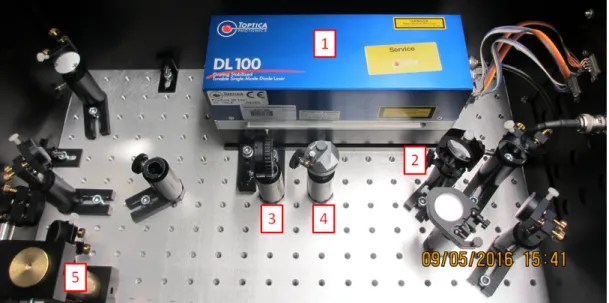
Figure 12: Laser system with removed plexi glass cover. 1) diode laser, 2) flip mount beamsplitter, 3) λ/2-plate, 4) polarizing beam splitter (PBS), 5) periscope to lower the laser beam level to the spectrometer level without changing its polarization.

Figure 13: K-cell to observe the fluorescence. Heating up the cell should only be done covering this division. Otherwise the K-cell will not heat up properly and not establish a high enough vapor

(21)

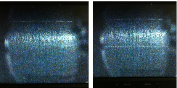
Figure 14: On the left: Laser detuned from correct frequency, no fluorescence signal. On the right: Laser tuned to the correct frequency, visible fluorescence signal.

3.1.1 Operating the laser

Turn on the laser driverToptica DL110 by turning on the mains switch. The temperature control will now heat up the laser diode to the set temperature. Wait for at least 30 Minutes now to be sure the whole laser system is in thermal equilibrium. It is recommended to leave the mains switch on during your whole one week/ two week experiment.

By pushing the green module on button above the mains switch the laser will start emitting. On the display above you can see the present settings for current and temperature of the diode. You can change the current by turning the ten turn potentiometer in theCurrent Control unit.

TheScan Control unit on the left is responsible for the feed forward of the laser. By turning theoffset adjustpotentiometer one can tilt the grating and simultaneously change the laser diode current in a fixed ratio. This distinctly increases the mode hop free tunability. Theamplitude potentiometer automatically ramps through the grating angle and the laser diode current with a sawtooth signal. This amplitude potentiometer is very helpful once you try to set the laser on the right frequency cause it will make the laser sweep over interval of frequencies.

One can vary the set temperature with the ten turn potentiometer at the temperature control unit. Be aware to change the temperature only in very small steps and take care that the system is in thermal equilibrium (i.e. wait 2 minutes per 0.1^◦C step) before you start turning at the current or grating angle potentiometers. A temperature of 24.9^◦C proved to be optimal to obtain a stable frequency. It is recommended not to change the temperature unless you didn’t try all other options, namely changing the laser diode current and the offset of the scan control iteratively. It can be very tricky to set the right frequency.

3.2 Vacuum System

To have a long enough mean free path for the electrons or ions produced in the experiment it is necessary to have a sufficiently high vacuum. Furthermore the MCPs in front of the detector need a vacuum of at least 10⁻⁶mbar in operation, otherwise they will be destroyed due to electrical discharges of possible contamination in the micro channels. When you begin with your measurements the pressure should be below 5·10⁻⁷mbar. To establish this high vacuum condition we use a combined integrated system of a scroll pump and a turbo-molecular pump. The scroll pump ensures a low enough pressure so that

(22)

Figure 15: The Laser is driven by the Toptica DL110 driver unit. 1) is the scan control responsible for the feed forward with the potentiometers for offset and amplitude of the sweeping mode.

2) is the temperature control unit 3) is the current control unit 4) is the mains switch and the switches to turn the laser on and off.

the turbo-molecular pump can start operation and establish the high vacuum conditions we need in this experiment. You can check on the pressure in the chamber using the programAgilent T-Plus.

3.3 Potassium oven

To have a thermal beam of Potassium it is necessary to heat up solid state Potassium to a temperature where its vapor pressure is high enough. The heat is supplied by twoFirerodcartrige heaters mounted in a copper clamp which is wrapped around the steel container with the Potassium in it. The temperature must not exceed 170^◦C. Of course we want a well collimated beam of atoms. Therefore the oven chamber has a small hole (2mm diameter) in direction of the interaction area with the laser. The metal around this small hole is cooled by a radiator. This makes the atoms condense at the cold walls, and only atoms with a well defined velocity vector can leave the oven chamber through the hole. The potassium beam has a diameter of roundabout 3.5mm in the interaction region with the laser.

Figure 16: The temperature control. Left site: K-oven, right site: K-cell

3.4 Atom Beam Detector

On the opposite side of the oven aLangmuir-Taylor-detector has its place. It is a very simple detector for alkali atoms. A glowing Rhenium filament ionizes the atoms that strike the filament via surface ionization. This happens between two electrodes of which one has hole. These plates apply an electrical field in the ionization volume. With this field the ions are accelerated towards a Faraday cup where the resulting current can be measured with a femtoamperemeter. Due to the high efficiency of the detector (nearly 100% of ions that strike the filament get ionized) the intensity of the beam can be calculated knowing the area of the filament.

3.5 CCD Camera and pBasex

(23)

The camera is mounted on top of the spectrometer as seen in fig 17. Be sure to focus the camera properly onto the phosphor surface and to mount the CCD surface parallel to the phosphor screen surface. Otherwise you will get systematically blurred and/or distorted pictures.

You can disassemble the camera from its mounting and use it as a beam profiler for the laser beam in combination with a quadrille paper.

Figure 17: The CCD camera mounted on top of the detector stage.

The programpBasexLis responsible for the inversion of the images of the detector surface in this experiment. A manual for the program is provided in the experiments folder on the PC provided. pBasexLis a program that handles the inverse Abel-transformation of a picture using the pBasex-Algorithm [8]. It displays the given velocity distribution and calculates theβ-coefficients for this distribution.

The settings for our application are: Set the ordernLof the used Legendre-polynomials to 4. Check the BoxSymY and uncheck the box Odd. Therefore only the Legendre-PolynomialsP0,P2 and P4 will be used to calculate the Θ-distribution, hence giving you the anisotropy parametersβ2andβ4.

(24)

pBasexL will give you a photoelectron velocity spectrum (PES). The x-Axis is the velocity of the electrons in pixels. The y-Axis is a intensity-axis in arbitrary units.

3.6 Power supplies

Here you can find an overview of all the electric power supplies.

Figure 18: The HV for the extractor and repeller electrode is provided by an HV-supply and split up by an adjustable HV-divider. 1) & 2) are the outputs for the repeller and extractor electrodes respectively. With 3) you can choose the ratioU_E/U_R. 4) is the input of the divider. The voltage is supplied by the fug HV-supply. One can adjust it with 5) (Voltage) and 6) (Current). Keep the current-poti as low as possible for safety reasons. With 7) you can switch polarity of the HV. Do this only while the HV-supply is shut down.

Figure 19: This is the HV-supply for the MCP. 1) & 2) are for coarse tuning and 3) for fine tuning. Use the smallest voltage you need for a sufficient signal due to saturation effects of the MCP.

(25)

Figure 20: This is the HV-Supply for the phosphor screen. You turn it on with the mains switch 1). Be sure the potis coarse and fine are completely turned down. Push the button 2) EHT. This will establish HV at the output. Now you can adjust the voltage using the potis. Do not exceed 4kV. Do not exceed a difference between MCP and phosphor voltage of 3kV.

Figure 21: The interlock module is built in to protect the detector stage from damage resulting from sudden pressure rise in the chamber. Its input voltage is given by the vacuum pump and depends linearly on the pressure in the chamber. If now the pressure rises above a certain value the interlock module cuts out the 220V supply for the HV-supplies. Therefore no damage can occur to the electrodes and the detector stage due to high pressure in the chamber. The interlock module is adjusted properly by the assistant.

Figure 22: On top you can see the Femtoamperemeter. Below there is the supply for the electrodes of the atom beam detector. 1) is for the extractor and 2) for the repeller.

(26)

Figure 23: Supply for the Re-filament. 1) & 2) are the voltage potis and 3) & 4) are the current settings, coarse and fine respectively. A current of 2A shall be applied to the Re-ribbon. Turn off the voltage current through the ribbon unless you need it. It heats up and cools down very quickly.

Do not exceed a current of 2A due to melting the Re-filament

Figure 24: This is the supply for the K-oven. Turning the yellow big knob will apply voltage.

(27)

Figure 25: This element supplies the voltage needed for the camera and the TFT-screen.

(28)

4 Simulations

4.1 The Poisson Equation

To get a better understanding of the fields acting on the ions or electrons in the spectrometer it is helpful to do some simulations first. The program SimIon can calculate the potential φ in a certain volume given by a certain (charged) spatial geometry. This problem is mathematically described by the Poisson equation:

−∆Φ = 4πρ inV (28)

withρ=ρ0 on∂V (29)

where ρ is a charge distribution. If there are no free charges in the volume V the Poisson equation reduces to the Laplace equation:

−∆Φ = 0 in V (30)

withρ=ρ₀ on∂V (31)

This equation is being numerically solved by SimIon using finite elements. The acceleration on a particle with chargeqby an electrical fieldE~ at a spatial point~ris given by:

~a(~r) = q m

E(~~ r) =−q

m∇Φ(~r) (32)

With the help of the known initial values for the velocity and the starting point the trajectories of the particle can be determined.

4.2 SimIon

A quick start guide for SimIon is provided in the Appendix. Make yourself familiar with the program.

Your goal will be to simulate the things going on in the spectrometer. The settings obtained in this simulation will be the initial values in your further measurements with the spectrometer. Therefore you may solve following problems:

Fly charged particles and observe their trajectories for different mass, charge, initial velocity and spatial values,U_E andU_R.

Find out the optimal ratio UE/UR of repeller and extractor electrode voltage for velocity map imaging. Therefore place two electrons in the ionization volume (center of the ionization volume isO~ = (0,0,0)) between the electrodes with identic velocity vectors but different spatial starting points (e.g. 1mm distance between them). Set the repeller voltage to 3kV. Plot the ratio of the impact distance on the detector and the initial distance ∆x^Det/∆xⁱⁿⁱvs. the ratio UE/UR. Adjust the extractor voltage in a way that the distance of the particles on the detector surface is minimized. Does this also work for differentU_R keeping the ratio U_E/U_Rconstant?

Set the voltages to the optimal ratio you determined above. Simulate a bunch of electrons (about 500) leaving the ionization volume with spherically distributed velocity vectors and one (two, three) defined kinetic energy. Explain what you see. Optional Determine the radius of the filled circle you see on the detector surface. How does the radius depend on the kinetic energy?

How does the repeller voltage (keeping the ratioUE/UR constant) affect the radius?

Switch to spatial map imaging by simulating K-ions. SetUR = 3kV. Place two atoms in

(29)

Optional Simulate a particle cloud that represents the ionization volume. Therefore calculate the rayleigh length zR and the beam waist w0 of the laser beam after a lens with f = 150mm assuming a 2σdiameter of the laser beam ofd= 1mm in front of the lens. Set the repeller voltage to 3kV. Find the optimal ratioUE/UR for spatial map imaging by minimizing the FWHM of the K-ion cloud mapped on the detector surface.

5 Measurements

5.1 The Laser

Tasks and Measurements:

1. Tune the laser to the correct frequency 2. Determine the focal volume of the laser beam 3. Mount the camera on the detector

Your first task is totune the laser to the correct frequency. To check if the laser is tuned to the correct frequency you may have a look at the fluorescence signal of the spectroscopy cell provided on the TFT-Screen. The camera is focused into the cell in a way that one can see the laser induced fluorescence of the K-atoms in the cell. Letting the laser sweep with the help of theamplitude potentiometer and trying different current settings may help to find the right frequency. When you observe a flicker of the fluorescence in the cell you know you are close to the right frequency. Now reduce the amplitude of the sweep and try to establish a stable fluorescence signal as in fig. 14. This is an iterative process.

Todetermine the focal volume of the laser beamit is necessary to know the diameter of the beam right before it is focused through the lens. Therefore one can take the CCD camera provided and set it up behind a quadrille paper. Taking pictures of the laser shining on the other side of the paper and by fitting Gauss-peaks at the intensity distribution one can obtain the diameter of the beam. Make sure that you measure within the dynamic range of the camera to avoid saturation.

Mount the camera onto the detectorand focus it on the phosphor screen. Install the light cover panel so that no scattered light can shine on the camera. Disconnect the wires for the HV Supply only at the light cover panel, not at the feedthroughs to the vacuum chamber. Switch all HV Supplys off when you do this.

5.2 Setting up the beam paths

1. Couple the laser into the K-Cell 2. Couple the laser into the Spectrometer

3. Establish the right polarization of the laser beam

Lift up the plexi glass covers over the laser and the K-cell. Adjust the laser beam by turning the micrometer screws at the mirrors. At first couple the beam into the K-cell. Right after that couple the beam into the spectrometerusing the entrance and exit windows. Use the flip mirror to decide whether the beam is coupled in at right angles to the atomic beam or in a counter propagating fashion. Take care not to hit the Re-Filament with the laser due to uncontrollable reflections.

Establish the right polarization of the laser beamwith the help of the λ/2 wave plate and the PBS. Which polarization do you want the laser beam to have?

(30)

5.3 Atom Beam Detector

1. Heat up the K-oven

2. Estabilsh the proper atom beam detector voltage settings 3. Measure the atomic flux vs. the oven temperature

Heat up the oven to a proper temperature. The permissible temperature of the oven reaches up to 170^◦C at 33 V heater voltage. Do not exceed this temperature, because too many K-Atoms effuse out of solid state and metallize the exit of the oven which causes a decreased atomic flux. Useful signals can be obtained around 140^◦C. The temperature is measured at the back of the oven chamber.

To start the operation of the atom beam detector set the current through the Re-filament toIRe= 2A.

The Re-filament will glow red at this current. Do not exceed this current cause you will melt and hence destroy the filament at higher currents. Wait about 10min. to be sure all pollution that may sit on the Re-filament gases out. Now carefully vary the repeller and extractor voltages (0-30V) until you find a maximum current measured by the femtoamperemeter. This is an iterative process. Make sure that the repeller voltage is always positive, whereas the extractor voltage is negative to yield an potential accelerating the ions towards the faraday-cup. Be careful to choose the right range on the femtoamperemeter.

Measure the atomic flux vs. the oven temperature. Try different oven temperatures within a the permissible range. Take care the system takes some time (min. 10 min) to reach thermal equilibrium after each change of temperature.

Discuss uncertainties and systematics of your results.

5.4 Obtaining first images with the spectrometer

1. Set the voltagesU_R andU_E,U_MCP andU_{P h} to the proper values 2. Take the CCD camera into operation

3. Focus the laser into the atomic beam

4. Tune the laser to the right frequency (fine tuning) 5. Optimize the signal

To obtain first images with the spectrometer it is useful to start with spatial map imaging of ions. At first you have to set the spectrometer electrodes to the correct voltages. Therefore you may use the voltage divider provided in the rack in combination with a HV-supply. To image ions you may set the HV-supply to positive polarity. Do only switch polarity whilst the HV-supply is turned off. Set the input of the voltage divider toUin= 3kV. This will also be the voltageUR applied at the repeller electrode. With the potentiometer you can tune the voltage at the extractor electrode in a range from 65% to 95%. Use your values from the simulation as initial values for the voltages.

Set the voltages at the MCP and the Phosphor screen to proper values. One can operate the MCP in a range of UMCP = 900V - 1050V. Generally you should choose the minimum necessary operation voltage to be sure not to saturate the MCP. The phosphor screen can be operated atUP h= 3- 4kV, but the difference betweenU_MCPandU_{P h}never may exceed 3kV. Take care of this limit when you turn off the detector: first turn down the voltage at the phosphor screen, then turn down the voltage at the MCP.

Take the CCD camera into operation. Run the programPylon View and select the camera. Click oncontinuous shot mode. To identify even very weak signals it may be necessary to set the camera to

(31)

in the Potassium beam compared to the broadening in the spectroscopy cell it will be harder to set the laser on the correct frequency. Very thoughtful adjustment of the feed-forward-offset will be necessary.

What you will see in the picture of the CCD camera is the focal area of the Laser beam crossing the atomic vapor beam. Optimize the signal obtained by the camera. Questions you should ask yourself during this iterative process: Is the laser at the right frequency? Is the laser properly focused into the interaction region with the K-beam? Is the ratioUE/UR set properly? Is the camera or the detector saturated? Do you have the right settings on the CCD camera? Is the camera exactly focused onto the phosphor screen? What is the signal to noise ratio?

5.5 Spatial Map Imaging with Ions

1. Determine the image ratio

2. Determine the optimal ratioUE/UR for spatial map imaging 3. Determine the dimensions of the focal area

4. Optional Determine the K-Beam diameter

5. Optional Check how the ionization rate depends on the laser power

Once you have a satisfying image you can start with your measurements. By translating the lens transversally to the propagation direction of the laser one can shift the focal area of the laser in the same way. One can now fit Gaussian peaks to the obtained pictures anddetermine the image ratio with the help of the peak position and the known translation of the lens.

Check how the beam waist of the focal area varies while you change the ratioUE/UR. Therefore make fits transverse to the profile of the laser focus. Determine the optimal ratio UE/UR for spatial map imaging. What kind of fit function will you need? How does the behavior of the measurement fit the expectations you got from the simulations?

The known image ratio and the optimal ratioUE/URcan now be used todetermine the dimensions of the laser focal area, namely the beam waist w0 and the Rayleigh lengthz0. Compare this value with your calculations and simulations.

Optional Find a way todetermine the diameter of the K-Beamusing this setup.

Optional Find away tocheck how the ionization rate depends on the laser power. What kind of relation do you expect? Hints: Use the variable attenuator to attenuate the laser beam entering the spectrometer. In this measurement the laser has to be absolutely stable.

5.6 Velocity Map Imaging with Electrons

1. Find the optimal ratioUE/UR for velocity map imaging 2. Record photoelectron spectra

3. Calibrate the energy axis

4. Determine the energy of the other K-States 5. Determine the resolution of the spectra 6. Determine the anisotropy parameters

7. Optional Explain the different peak intensities

8. Optional Check how the radius of the rings depends on the repeller voltageUR

To image electrons with the detector you have to change the polarity on the electrodes to negative. Do this only when the HV-Supply is turned off.

(32)

Set the ratioU_E/U_R to the value you determined in your simulations. All the other settings of section 5.5can be retained. Take pictures at different ratiosUE/UR, calculate the FWHM of the peaks andfind the optimal ratio(i.e. the minimum of the FWHM) for your further measurements. Is this consistent with the results of your simulation?

Record photoelectron spectra (PES) of Potassium with the optimal settings you determined above. Invert them with the program pBasex. Transform the obtained PES into an energy spectrum using that the kinetic energy is proportional to the squared velocity: Ekin =kv². Take care to use the correct jacobians during the transformationP_v(v)→P_E(E).

Calibrate the energy axisusing the known ionization threshold and the laser wavelength.

Determine the energies of the other peaksand identify them with the help of the level scheme of Potassium. How many peaks did you naively expect?

Determine the resolution of the spectra. Therefore compare the size of a single event on the detector with the FWHM of the peaks. Which effects contribute more, which effects contribute less to the limitation of the resolution?

pBasexL also determines theanisotropy parametersβ₂ andβ₄over the radius of the given distribution. Determine the anisotropy parameters by weighting them with the intensity-axis of the PES and averaging them over the FWHM of the peaks. This method has proven to be appropriate for the calcu- lation of the parameters. Compare the calculated parameters to the pictures (e.g. Plot the distribution J_n,l(Θ) = 1 +β₂P₂(cos Θ) +β₄P₄(cos Θ) and cross-check it with the obtained images.

Optional Explain the different peak intensitiesusing a rate equation model and the known ionization cross-sections as shown in sec. 2.4.4.

Optional Check how the radius of the rings depends on the repeller voltage UR, leaving the ratioUE/UR at a constant value. You can vary this voltage with the HV-supply in a broad range from 0kV to 5kV.

5.7 VMI Ions with transversal laser incoupling

1. Optional Record velocity spectra of K-ions

2. Optional Determine the velocity spectrum of the K-ions

Imaging K-ions in the VMI-mode generates a velocity distribution of the K-ions. Therefore you may use the same ratio of voltages at the electrodes you used with the VMI-electrons, but of course you have to change the polarity. Turn down the HV-supply before you switch the polarity. The distribution of the velocities of the ions in the oven is well described by a Maxwell-Boltzmann distribution:

f(v)dv= 4π m

2πk_BT ^3/2

v²exp

− m 2k_bTv²

dv (33)

The signal obtained for a certain velocity meaning the intensity on a certain point of the detector is proportional to the following equation:

(33)

Fitting this function to the obtained velocity distribution will give you the inner temperature of the oven. To calibrate the velocity-axis you may use either the known calibration of the electrons or results from simulations. Take care that the oven reaches thermal equilibrium after changing the temperature.

This may take at least half an hour.

(34)

6 Notes and Safety Notes

This experiment is very sensitive to faulty operation and severe damage can occur to elementary parts of the setup. If you take care of the notes and limits denoted below damage to the setup by faulty operation can be excluded.

6.1 High Voltages

The correct sequence to apply the HV is: 1) MCP, 2) Phosphor Screen, 3) VMI Electrodes.

The maximum voltage on the MCP is 1050V

The maximum voltage for the Phosphor screen is 4kV

The maximum voltage for the voltage divider (UR, UE) is 5kV

The maximum difference betweenU_MCP andU_Phis 3kV. Be careful when applying voltages to the Phosphor screen and to the MCP not to exceed this limit.

Turn down all high voltages when you don’t need them for a longer time. The correct sequence for turning them down is: 1) VMI Electrodes, 2) Phosphor Screen, 3) MCP.

Turn down high voltage before you switch its polarity

To focus the camera onto the phosphor screen disconnect the wires for the HV supply only at the light cover panel, not at the feedthroughs to the vacuum chamber. Switch all HV supplies off when you do this.

6.2 Temperatures

The maximum temperature at the K-cell is: 160^◦C

The maximum temperature at the K-oven is: 170^◦C

6.3 Pressure

The pressure in the chamber must be below 5·10⁻⁷mbar to take the spectrometer into operation.

6.4 Atomic Beam Detector

Do not apply a current over 2A to the Re-filament due to melting it. After applying voltage to the Re-filament wait for 10 minutes. This ensures that possible pollution on the filament gases out.

If you decrease the voltage at the supply for the atomic beam detector electrodes this takes some time (approx. 20s). Take care of this effect when you optimize the voltages for your atomic flux measurement.

6.5 Miscellaneous

Block the laser before it enters the spectrometer unless you need it for experiments.

...

(35)

A Appendix

A.1 Getting started with Simion

Open the program SimIon 8. You can find it in the experiments folder . Follow the instructions in the given screen shots.

Figure 26: The program wants you to load a geometry file which you can find in the folder vmi, its name is geometry.iob.

(36)

Figure 27: Here one can see the setup of the spectrometer. On the left side the three electrodes of which two have a hole in it to let the particles pass through. Namely there are repeller- extractor- and ground-electrode (from left to right). At the right end of the spectrometer one can see the detector. Use the marked tabs to navigate through the program.

(37)

Figure 28: Select the Tab Particles. Be sure that the checks are set in the same way as in the screenshot. By clicking on the Define button you can define the particles you want to do the simulations with. Hitting the button Data Recording provides the settings for data recording. In your case it is sufficient to record the particle position at the moment it hits the detector.

(38)

Figure 29: In this menu you can modify the particles you want to do the simulations with. You can group them in various groups and choose their properties like charge, spatial starting point, starting velocity and direction, etc. One can even choose a spatial- or velocity-distributions of the particles with the help of this menu. The ionization volume has the coordinates (0,0,0) in the coordinate system of the program. Save your simulated particles and click on the OK. button to use these particles.

(39)

Figure 30: Hitting the tab PAs and then the button Fast Adjust Voltages... you can apply voltages to the repeller and extractor electrodes. Click on Fast Adjust to feed the program with this settings.

(40)

Figure 31: Hitting the tab PE/Contours, checking the box Draw and setting the Auto button to 10 e.g. you can see the equipotential lines given by the field in the spectrometer. Now you can finally push the button Fly’m and obtain the particles’ trajectories. You can obtain the log file of the simulations with the data you selected in Data Recording under the tab Log. This can be used for further calculations.

(41)

A.2 Using Mathematica for Image Processing and Evaluation

In order to process the image data you observed during your measurements it is helpful to use the provided Mathematica notebook ImageProcessing.nb for starters. You can find it in the experiments folder.

A.3 Pylon Viewer

Connect the Camera via the USB 3.0 Card on the backside of the PC and on the backside of the camera.

Open the programPylon Viewer

Figure 32: Double-click on the camera to select it.

(42)

Figure 33: Click on Continuous shot mode to record continuous shots with the CCD camera.

Use the buttons on the right to adjust the image.

(43)

Figure 34: Open the camera settings. Under Analog Control one can change the parameters for gain, gamma and the black level. Under Acquisition Control one can change the exposure time and the repetition rate of the camera.

(44)

Figure 35: Set the exposure time settings to reasonable values. It may be necessary to change these values sometimes during the experiment, for example at first it is important to see even small signals but for measurement it is important to have a good signal to noise ratio.

(45)

References

[1] Christof Bartels. Angular distributions of photoelectrons from cold, size-selected sodium cluster an- ions. PhD thesis, Albert-Ludwigs-Universit¨at Freiburg, 2008. Available athttps://www.freidok.

uni-freiburg.de/data/5241.

[2] Jwei-Jun Chang and Hugh P. Kelly. Relativistic calculations for photoionization cross sections and the spin orientation of photoejected electrons from potassium, rubidium, and cesium atoms. Phys.

Rev. A, 5:1713–1717, Apr 1972.

[3] J Cooper and R.N.. Zare. Angular distribution of photoelectrons. J. Chem. Phys., 48:942–943, 1968.

[4] Wolfgang Demtr¨oder. Laser Spectroscopy - Basic Concepts and Instrumentation. Springer Science

& Business Media, Berlin Heidelberg, 3rd ed. edition, 2002.

[5] Wolfgang Demtr¨oder. Experimentalphysik 2 (3., Berarb. U. Erw. Aufl. 200) -. Springer, Berlin, Heidelberg, 3rd edition, 2004.

[6] Andre T. J. B. Eppink and David H. Parker. Velocity map imaging of ions and electrons using electrostatic lenses: Application in photoelectron and photofragment ion imaging of molecular oxygen.

Review of scientific Instruments, 68(9):3477–3484, 1997.

[7] Lutz Fechner. Aufbau eines velocity-map-imaging-spektrometers und winkelaufgel¨oste spektroskopie an rubidium-dotierten helium-nanotr¨opfchen, 2011. Availability: Ask your assistant.

[8] Gustavo A. Garcia, Laurent Nahon, and Ivan Powis. Two-dimensional charged particle image inversion using a polar basis function expansion. Review of Scientific Instruments, 75(11):4989–

4996, 2004.

[9] Dieter Meschede.Optics, Light and Lasers - The Practical Approach to Modern Aspects of Photonics and Laser Physics. John Wiley and Sons, New York, 2008.

[10] W. Sandner, T. F. Gallagher, K. A. Safinya, and F. Gounand. Photoionization of potassium in the vicinity of the minimum in the cross section. Phys. Rev. A, 23:2732–2735, May 1981.

[11] T. G. Tiecke. Properties of potassium, 2011. Available athttp://www.tobiastiecke.nl/archive/

PotassiumProperties.pdf.