Global teleconnections associated with diabatic heating due to local rainfall events

Global teleconnections associated with diabatic heating due to local rainfall events

Master Thesis

submitted in fulfilment of the requirements for the degree

Master of Science (M. Sc.)

Climate Physics: Meteorology and Physical Oceanography

Faculty of Mathematics and Natural Sciences Christian – Albrechts – Universität zu Kiel

Sandro Dahlke 954253

Supervisor: Prof. Dr. Richard Greatbatch Second Supervisor: Prof. Dr. Katja Matthes

Kiel, August 2015

Abstract

In this thesis, atmospheric teleconnection patterns and their interannual connection to anomalous local rainfall in the summer and winter season are investigated in the period af- ter 1979. Given the lack of quality of gridded reanalysis rainfall products, especially in the period prior to 1979, an ensemble mean estimate of three satellite-based rainfall products cov- ering 32 years is used as a proxy for diabatic heating in the troposphere. It is shown that the diabatic heating due to local rainfall can affect the tropospheric circulation in regions very distant from the heating, while the induced teleconnections may as well affect global weather and climate. It is argued that planetary waves are responsible for communicating the tele- connections throughout the globe. Hence, anomalous Rossby Wave Sources (RWSs), that are related to the diabatic heating, are shown to drive the teleconnection patterns via generation of vorticity. It is found that the midlatitude jets play an important role for the generation of teleconnections, as they act as waveguides for planetary waves.

The satellite ensemble mean rainfall in the tropical Pacific has good skill in reproducing tele- connections that are associated with El Niño, namely the projection onto the Pacific North American (PNA) pattern and the Pacific South American (PSA) pattern.

It is shown that even when the signal of El Niño and the local SST is removed from the sea- sonal rainfall everywhere on the globe, there are regions evident, where anomalous rainfall can disturb the troposphere and generate global-scale teleconnections. Thus, anomalous diabatic heating over the central Pacific Ocean generates a westward shifted PNA pattern.

Further, enhanced winter rainfall over the tropical Indian Ocean projects onto the positive phase of the North Atlantic Oscillation (NAO), which is the dominant mode of atmospheric variability over the Atlantic sector. This finding implies a remote impact of the convective activity over the Indian Ocean on European Climate.

Interannual variability of diabatic heating during the Indian Summer Monsoon (ISM) drives a circumglobal teleconnection pattern in the northern hemisphere. This pattern in turn affects climate and rainfall in several regions of the world, especially in northeast China and northern Africa.

The results further suggest that teleconnection patterns associated with anomalous rainfall over the Tropical Indian Ocean, the Maritime Continent, the Indian peninsula and the Gulf Stream, bear similarities to the circumpolar wavetrain discussed in Branstator (2002).

In the tropics, the atmospheric response to diabatic heating resembles the Gill-type response, emphasizing that the satellite ensemble mean rainfall is a good representation of diabatic heat- ing in the last 32 years.

Zusammenfassung

In dieser Arbeit werden atmosphärische Telekonnektionen auf ihre interannuelle Verbindung zu lokaler Niederschlagsvariabilität in den Sommern und Wintern nach 1979 untersucht. We- gen der Qualitätsprobleme von Reanalyseniederschlägen, insbesondere in der Zeit vor 1979, wird das Mittel aus drei unabhängigen satellitengestützten Niederschlagsprodukten berechnet.

DiesesEnsemblemitteldeckt 32 Jahre ab und wird als ein Proxy für diabatische Erwärmung in der Troposphäre verwendet. Es wird gezeigt, dass die diabatische Erwärmung, die bei starkem Niederschlag auftritt, die Zirkulation in der Troposphäre selbst in Regionen beeinflussen kann, die weit entfernt sind von der Region des erhöhten Niederschlages. Die dabei erzeugten Telekonnektionen können ihrerseits das globale Klima und Wetter beeinflussen. Planetare Wellen sind für die Generierung der Telekonnektionen verantwortlich, was durch eine Anal- yse der Rossby Wave Source (RWS) gezeigt wird, die Vorticity generiert. Dabei spielen die Strahlströme in mittleren Breiten eine wichtige Rolle bei der Erzeugung von Telekonnektio- nen, da sie als Wellenleiter für planetare Wellen fungieren.

Im tropischen Pazifik reproduziert der Niederschlag des Ensemblemittels sehr gut die Telekon- nektionen, die mit El Niño assoziiert werden. Diese sind das Pacific North American (PNA) pattern und das Pacific South American (PSA) pattern.

Darüber hinaus wird gezeigt, dass selbst dann noch Regionen existieren, in denen erhöhter Niederschlag die globale Atmosphärenzirkulation antreibt, wenn das Signal von El Niño und das der lokalen Meeresoberflächentemperatur entfernt wird.

Im Winter projiziert erhöhter Niederschlag über dem tropischen Indischen Ozean auf die pos- itive Phase der Nordatlantischen Oszillation (NAO), welche die dominante Mode der Kli- mavariabilität über dem Atlantischen Sektor ist. Dieses Ergebnis impliziert, dass Konvek- tionsaktivität über dem Indischen Ozean das Klima in Europa beeinflusst.

Interannuelle Variabilität in der diabatischen Atmosphärenerwärmung während des Indischen Sommermonsuns (ISM) erzeugt eine zirkumglobale Telekonnektion in der nördlichen Hemis- phäre. Diese Telekonnektion übt wiederum einen signifikanten Einfluss auf das Klima und den Niederschlag in weiten Teilen der Welt aus, insbesondere im Nordosten Chinas und in Nordafrika.

Des Weiteren deuten die Ergebnisse darauf hin, dass die Telekonnektionen, die in Verbindung stehen mit erhöhtem Niederschlag über dem Indischen Ozean, dem Maritimen Kontinent, In- dien und über dem Golfstrom, den zirkumpolaren Wellenzug widerspiegeln, der in Branstator (2002) diskutiert wird.

In den Tropen ähnelt die atmosphärische Antwort auf diabatische Erwärmung der Gill-type response. Dies untermauert, dass der saisonale Niederschlag des Ensemblemittels für die Zeit von 1980 - 2011 eine gute Repräsentation der diabatischen Erwärmung in der Troposphäre ist.

Contents

1 Introduction 6

2 Data and methods 11

2.1 Rainfall data . . . 11

2.2 General rainfall analysis . . . 12

2.3 Removing the ENSO signal . . . 18

2.4 Atmospheric variables . . . 20

2.5 Documented recurrent teleconnection patterns . . . 21

2.6 Wave guides and Rossby wave source . . . 25

3 Tropical Pacific teleconnections 27 3.1 ENSO teleconnections . . . 27

ENSO stratospheric teleconnections . . . 31

3.2 Central Pacific teleconnections . . . 35

3.3 Maritime Continent teleconnections . . . 38

4 Indian Ocean boreal winter teleconnections 42 5 Gulf Stream boreal winter teleconnections 50 6 Indian Summer Monsoon teleconnections 53 6.1 Impacts of the ISM teleconnection . . . 57

The ISM - Sahara/Mediterranean link . . . 57

The ISM - North China link . . . 59

7 Summary and Conclusions 61

8 Acknowledgements 65

1 Introduction

1. Introduction

Figure 1:DJF monthly mean one-point correlation of 500 hPa geopotential height at the grid points a) 45^◦N, 165^◦W, b) 55^◦N, 20^◦W.

Contour interval is 0.2. a) closely resem- bles the PNA pattern, b) the EA pattern (from Wallace and Gutzler (1981)).

In atmospheric sciences, the term teleconnec- tiondescribes the tendency of atmospheric pa- rameters, in most cases geopotential height, but also temperature or wind speed, to show sim- ilar behaviour between geographically widely separated points throughout the globe. Tele- connections are large - scale, simultaneous interrelations between geographical locations and they are usually active on time scales of a week up to a season (Wallace and Gut- zler, 1981). Wallace and Gutzler (1981) as- sociate teleconnections with standing oscilla- tions in the troposphere geopotential height.

They analyse one-point correlation maps of the fields of geopotential height to reveal ge- ographically dependent, recurrent teleconnec- tion patterns. Figure 1 shows their correlation maps for two base points [45^◦N, 165^◦W] and [55^◦N, 20^◦W], obtained using the 45 winter months (DJF) from 1962/63 to 1976/77. One can clearly identify patterns consisting of well- separated patches of different amplitude. Wal- lace and Gutzler (1981) name these particular patterns the Pacific North American (PNA) pat- tern (top panel) and the East Atlantic (EA) pat-

tern (lower panel). Another way to find dominant patterns of low frequency variability in the atmospheric circulation is to carry out an Empirical Orthogonal Function analysis (EOF, see von Storch and Zwiers (1999) for details). EOFs of sea level pressure (SLP) or geopotential height at a certain pressure level are used in many studies to detect circulation regimes in a domain of interest (Mo and Peagle, 2001, Hurrell et al., 2003, Sun et al., 2010, amongst many others). Several exam- ples of prominent teleconnection patterns, including those which will be mentioned in this thesis, are described and defined in section 2.5.

1 Introduction

Teleconnections are of large scientific and socio-economic interest since the variability of the atmospheric circulation associated with teleconnections is known to affect the weather in many regions of the world. For example, winter rainfall in Western Europe and Scandinavia is strongly dependent on the state of the North Atlantic Oscillation (NAO), since it determines the strength of the midlatitude westerly winds across Europe that advect moist marine air masses from the At- lantic (Greatbatch, 2000, Hurrell et al., 2003).

Another example demonstrating how atmospheric circulation can affect local rainfall is given by Mo and Peagle (2001), who point out the role of the Pacific-South American (PSA) pattern in modulating rainfall over South America. This motivates the investigation of what drives such low frequency (interannual), recurrent atmospheric teleconnection patterns. Are they purely internal variability in the climate system arising from eddy-mean flow interaction, or may they be excited by a local forcing of the atmosphere, such as enhanced diabatic heating, which occurs in times of excessive rainfall and thus anomalous deep convection? Nowadays, it is widely believed that many prominent teleconnections appear as the atmospheric response to deep convection caused by the slowly varying tropical SSTs (Trenberth et al., 1998), but one must note that there may also be regions where strong convective activity is found, that can drive the atmosphere without being necessarily related to the underlying SST. Using observational data alone, one is limited in de- tecting and distinguishing between different driving mechanisms for the atmosphere. Thus, there are many studies analysing the atmospheric response to an imposed local forcing using General Circulation Models [GCMs, (e.g. Hoskins and Karoly, 1981)] or simple vorticity balance models (Sardeshmukh and Hoskins, 1988). Hoskins and Karoly (1981), for example, point out that a lin- ear baroclinic model of the atmosphere can exert global scale wave trains for both thermal and orographic forcing.

While most classical studies used SST anomalies as forcing, nowadays it has also proven equally effective to integrate the model with a specified general tropical heating source centred at a certain (tropospheric) level (Hoskins and Karoly, 1981, Sun et al., 2010, Greatbatch et al., 2013). Local sources of diabatic heating are shown to initiate global scale teleconnections (e.g. Hoskins and Karoly, 1981, Sardeshmukh and Hoskins, 1988, Lin, 2009). In the real world, these sources may be associated with strong local rainfall events, persisting sometimes over several months.

The general complication concerning the dynamical connection between rainfall and atmospheric

1 Introduction

circulation can nicely be illustrated when thinking again about the aforementioned PSA pattern and its correspondence to El Niño Southern Oscillation (ENSO). ENSO is a complex ocean - at- mosphere coupled phenomenon, that involves both SST anomalies along the central to eastern tropical Pacific and anomalous vertical motion in the Pacific domain. While assumed to affect South American rainfall via advection of moist air, the PSA pattern itself is thought to be the atmospheric response to ENSO in the Southern Hemisphere (Mo and Peagle, 2001), given the anomalous deep convection and rainfall in the eastern tropical Pacific during strong ENSO events.

To give an example for boreal summer, Greatbatch et al. (2013) suggest a dynamical response of the atmosphere to excessive rainfall in India during the Indian summer monsoon (ISM). This re- sponse in turn projects onto the second mode of variability of the wind field in an enclosed region over China, such that the atmospheric response finally leads to enhanced rainfall over northern China (Sun et al., 2010). Further, Ding and Wang (2005) point out that the ISM heating provides a possible forcing mechanism for a circumglobal teleconnection pattern, which in turn significantly affects rainfall in parts of Western Europe, Russia, North America and Asia. These examples demonstrate general difficulties in distinguishing, on an interannual basis, whether it is the atmo- sphere that drives the rainfall, or vice versa. Thus, understanding the associated relationships and causalities may yield improvements in predictability of climate in many regions of the world.

Hence, there are numerous studies to explain possible mechanisms for how a local forcing, like deep convection due to anomalous surface heating or latent heat release by anomalous rainfall, can induce atmospheric circulation changes. Using 3-hourly radiosonde data, Mitovski and Folkins (2014) show that during the 1-2 days period around a strong rainfall event, the troposphere near the rainfall region is significantly affected. In particular, positive geopotential height- and temperature anomalies are observed in the mid to upper troposphere (400 - 200 hPa), while negative geopo- tential height- and temperature anomalies prevail at lower levels. Mitovski and Folkins (2014) find these effects in the troposphere to extend 600-1000 km radially away from the location of the strong rainfall event.

Trenberth et al. (1998) point out the role of tropical surface forcing in producing tropical deep convection, which in turn strengthens the Walker- and Hadley circulation. In upper tropospheric levels this results in anomalous divergence of the meridional wind in the tropics and anomalous convergence at higher latitudes. Finally, these anomalies can act as a Rossby wave source and thus initiate the overall atmospheric response, even at latitudes far away from the forcing region (Sardeshmukh and Hoskins, 1988). They further claim that the longitudinal position of the tropical

1 Introduction

heating is essential to the actual response pattern, such that there exist some preferred pathways for teleconnective responses in the tropics.

The theoretical basis for the forcing of planetary waves in the tropics has its beginnings in the work of Matsuno (1970) and Gill (1980). Condensing the most important points from these stud- ies, the tropical response is governed by a fast Kelvin wave to the east of the forcing region and a slower Rossby wave response to the west. The equatorial Kelvin wave travels eastward, leaving anomalous low pressure in its wake at the surface and anomalous high pressure aloft. According to Gill (1980), the footprint of the slower westward propagating Rossby wave at the surface is given by two cyclones (anticyclones aloft), that are symmetric about the equator and are located slightly north- and south west of the forcing region. On the other hand side, for a response to penetrate out of the tropics, the overall existence of subtropical Rossby waves is crucial and therefore, genera- tion of a Rossby wave source in the subtropics is favourably (Sardeshmukh and Hoskins, 1988).

Further, the response in high latitudes becomes more and more barotropic, while in the Tropics, the response is rather baroclinic.

In the pioneering work of Wallace and Gutzler (1981) on teleconnections, there were only 15 years of geopotential height data available, which raises the question about reproducibility and stationar- ity of the teleconnections on longer time scales. The aim of this thesis is to further consolidate and examine atmospheric teleconnection patterns and their relation to local rainfall anomalies. There- fore, an ensemble of three satellite rainfall products for the last 32 years is used to investigate the effect of rainfall on the atmosphere. To our knowledge, this particular analysis has not been under- taken before.

The launch of rainfall measuring satellites in the 1970s greatly enhanced the quality of precipi- tation data, especially over the oceans, and enabled their availability as global gridded data (Arkin and Meisner, 1987, Efthymiadis et al., 2005). One must keep in mind that prior to the satellite era, observational precipitation data were restricted to land-based rain gauges and ship cruise measure- ments, both suffering temporal and spatial inhomogeneity.

The questionable quality of (tropical) rainfall in reanalysis data, especially in the pre - satellite era, is discussed, for example, in Poccard et al. (2000) and Efthymiadis et al. (2005). In Figure 2, local rainfall estimates of two reanalysis products (NCEP/NCAR and ERA40) are compared with CMAP satellite measured rainfall. It clearly depicts the discrepancies between reanalysis and

1 Introduction

1950 1960 1970 1980 1990 2000

−0.5 0 0.5 1

Nino3.4 precipitation

NCEP (1948−2008) E40 (1957−2002) CMAP (1979−2007)

1950 1960 1970 1980 1990 2000

−0.4

−0.2 0 0.2 0.4 0.6

South America precipitation

1950 1960 1970 1980 1990 2000

−0.5 0 0.5

Gulf Stream precipitation

1950 1960 1970 1980 1990 2000

−0.6

−0.4

−0.2 0 0.2 0.4

Congo precipitation

1950 1960 1970 1980 1990 2000

−0.6

−0.4

−0.2 0 0.2 0.4

Maritime Continent precipitation

0 50 100 150 200 250 300 350

−50 0 50

Figure 2:Some examples of normalized DJF mean rainfall anomalies for five regions of the world (see section 2 for details about the rainfall data and rainfall regions ). Shown are the values from both reanalysis NCEP (blue) and ERA40 (red), as well as CMAP satellite rainfall anomalies (black). Bottom right shows the position of the boxes.

CMAP in the satellite era, but also the discrepancies between the two reanalysis products in the pre- satellite era, especially in the tropics. There have been attempts to reconstruct pre - 1979 oceanic precipitation using land-based gauge data or reanalysis precipitation (Efthymiadis et al., 2005). The authors, however, find that the reconstruction skill is poor in regions far away from the coast and in years without ENSO activity. Since we are also interested in processes apart from ENSO, we decided to focus our study on rainfall data derived from satellite soundings (period after November 1979) and investigate their effect on the atmosphere. Thus, the data analysed here span a time of well above 30 years, which allows for confidence in the results, when using typi- cal statistical time series analysis methods to examine the relationship between local rainfall and teleconnections.

2 Data and methods

2. Data and methods

2.1. Rainfall data

Given the large discrepancies regarding tropical rainfall amongst different rainfall products (Figure 2), this study uses different satellite-based rainfall products, although this restricts the analysis to the period after 1979. This is reasonable, because the quality of NCEP/NCAR rainfall has been found to be very questionable in the pre-satellite era (Poccard et al., 2000, for example). On the other hand, the availability of satellite rainfall sensors, which operate at microwave and infra-red wavelengths, has dramatically improved both accuracy and spatial homogeneity of global rainfall data (see, for example, Arkin and Meisner, 1987, Todd and Washington, 1999).

Our aim is to average different rainfall products in the regions sketched in Figure 4 in order to generate an ensemble mean rainfall. We decided to use an ensemble of three independent satel- lite based rainfall data sets, which will be introduced in the following. One product is the Global Precipitation Climatology Project [GPCP, Adler et al. (2003)], which combines monthly satellite data with estimates from over 6,000 rain gauge stations, low-orbit infrared, passive microwave, and sounding observations. This provides a very complete analysis over the World Oceans, and adds additional information over land to increase accuracy. Data are available from 1979 to present at a spatial resolution of 2.5^◦. The second product used is CPC Merged Analysis of Precipitation [CMAP, Xie and Arkin (1997)], which contains monthly data from five kinds of satellite estimates (GPI,OPI,SSM/I scattering, SSM/I emission and MSU). Data are available from 1979 to present and are stored at 2.5^◦horizontal resolution. The third product used here is the Climate Anomaly Monitoring System (CAMS) and OLR Precipitation Index (OPI); see, for example, Janowiak and Xie (1999). This analysis combines OPI satellite rainfall estimates with data from rain gauges (CAMS) to get real-time monthly estimates of global precipitation on a 2.5^◦x 2.5^◦grid from 1979 to present. The termensemble mean, which is used in this study, refers to the mean of the GPCP, CMAP and CAMS/OPI precipitation.

Regarding the analysis of summertime rainfall, an additional rainfall product is used for the Indian region: the All India Rainfall Index (Parthasarathy et al., 1995). This dataset has the advantage of yielding uninterrupted rain gauge data from 2000 back to the year 1871. This enables a compari- son with atmospheric parameters from the early NCEP/NCAR reanalysis (post 1949). The dataset contains annual estimates for the cumulative June/July/August/September (JJAS) rainfall, taken

2 Data and methods 2.2 General rainfall analysis

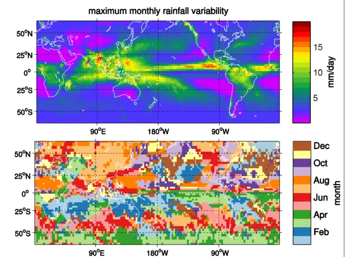
Figure 3:Maximum monthly mean rainfall variability. Shown is the highest standard deviation of the interannual monthly mean rainfall variability (top) and the corresponding month of the occur- rence of this maximum standard deviation (bottom)

from 306 stations in India. The authors claim that the number and distribution of rain gauges is consistent until 1990, but the number and distribution of rain gauges is unknown from 1991 - 2000.

2.2. General rainfall analysis

Figure 3 shows the maximum standard deviation of the interannual variability of monthly mean rainfall and the month of occurrence of the maximum in this standard deviation. The ensemble mean rainfall is used here. According to the map, several geographical boxes are chosen, where strong variability is found in the boreal winter time: The Central Pacific region (CP), the Maritime Continent (MC), The Gulf Stream (GU), the Tropical Indian Ocean (IO), the Tropical Eastern Pacific Nino region (Nino3.4 box) and the South America (SA) box. There are also regions where rainfall variability peaks in boreal summer. For this study, the regions of India (IND), Northern China (CH) and the Sahel are of particular interest. The exact geographical locations of these boxes are summed up in Table 1 and in Figure 4, respectively. A special case is the Congo (CO) box, where variability peaks in October/November, but further analysis (Figure 5) shows that the

2 Data and methods 2.2 General rainfall analysis

CP Nino3.4 IO MC

GU IND

CH Sahel

SA CO

longitude

latitude

rainfall boxes

0 50 100 150 200 250 300 350

−40

−20 0 20 40 60

Figure 4:Map showing the location of the boxes listed in Table 1.

Box ^◦lat ^◦lon

Nino3.4 5S - 5N 190E - 240E CP 10S - 10N 150E - 200E MC 10S - 5N 100E - 150E GU 32N - 42N 285E - 300E

IO 5S - 5N 70E - 80E

CO 5S - 5N 5E - 30E

IND 8N - 28N 72E - 88E CH 35N - 45N 105E - 120E Sahel 10N - 25N 358E - 32E Table 1:Geographical position of the rainfall boxes

which are considered in winter (top) or sum- mer (bottom), for the longitudinal and latitu- dinal limits, the first number is the western- most (southernmost) limit for each box seasonal cycle is dominated by a double-peak

structure in boreal spring and autumn, which is very likely the manifestation of the Intertropi- cal Convergence Zone (ITCZ), that crosses the equator twice a year and is associated with en- hanced rainfall. The seasonal cycle of precip- itation in these boxes, as well as its variabil- ity, is shown in Figure 5. It reveals regions of comparably low variability throughout the year (the three summer boxes IND, CH, Sahel, and IO) and regions with a strong seasonal cycle in terms of rainfall variability (e.g. Nino3.4, MC, CP). From Figure 5, it seems that strongest amounts of rainfall are likely to coincide with the month of strongest rainfallvariability. One exception from that is the Nino3.4 box, where

maximum rainfall occurs in boreal spring (MAM), while strongest variability is found in boreal winter (DJF). We thus conclude to restrict our analysis to DJF mean rainfall for the winter boxes and JJAS mean rainfall for the summer boxes (JJAS for enabling comparison with All India Rain- fall Index).

Accordingly, Figure 6 shows time series of DJF and JJAS rainfall, averaged in the correspond-

2 Data and methods 2.2 General rainfall analysis

J F M A M J J A S O N D 0

5 10

mm/day

Nino3.4

J F M A M J J A S O N D 0

5 10

mm/day

CP

J F M A M J J A S O N D 0

5 10

mm/day

SA

J F M A M J J A S O N D 0

5 10

mm/day

MC

J F M A M J J A S O N D 0

5 10

mm/day

GU

J F M A M J J A S O N D 0

5 10

mm/day

CO

J F M A M J J A S O N D 0

5 10

mm/day

Sahel

J F M A M J J A S O N D 0

5 10

mm/day

IO

J F M A M J J A S O N D 0

5 10

mm/day

IND

J F M A M J J A S O N D 0

5 10

mm/day

CH

2*std mean

Figure 5:Seasonal cycle (red curves) and 2·standard deviation (blue bars) of interannual monthly mean precipitation (seasonal cycle removed) in rainfall boxes using the satellite ensemble mean prod- uct from 1979-2011

2 Data and methods 2.2 General rainfall analysis

19800 1990 2000 2010 5

10

Nino3.4

mm/d

CMAP m= 2.09 sd= 2.53 CAMS m= 2.43 sd= 2.79 GPCP m= 2.3 sd= 2.82

19800 1990 2000 2010 5

10

CP

mm/d

CMAP m= 7.82 sd= 2.39 CAMS m= 7.37 sd= 2.75 GPCP m= 6.66 sd= 1.99

19800 1990 2000 2010 5

10

GU

mm/d

CMAP m= 5.45 sd= 0.64 CAMS m= 4.88 sd= 0.6 GPCP m= 6.02 sd= 0.7

19800 1990 2000 2010 5

10

MC

mm/d

CMAP m= 9.02 sd= 1.34 CAMS m= 8.87 sd= 1.32 GPCP m= 7.8 sd= 0.99

19800 1990 2000 2010 5

10

IO

mm/d

CMAP m= 6.17 sd= 1.44 CAMS m= 6.22 sd= 1.28 GPCP m= 4.82 sd= 1.2

19800 1990 2000 2010 2

4 6 8 10

IND

mm/d

CMAP m= 7.27 sd= 0.69 CAMS m= 7.37 sd= 0.71 GPCP m= 7.41 sd= 0.68

19800 1990 2000 2010 2

4 6 8 10

CH

mm/d

CMAP m= 2.19 sd= 0.28 CAMS m= 2.19 sd= 0.28 GPCP m= 2.35 sd= 0.32

19800 1990 2000 2010 2

4 6 8 10

CO

mm/d

CMAP m= 4.18 sd= 0.49 CAMS m= 4.09 sd= 0.53 GPCP m= 3.76 sd= 0.36

19800 1990 2000 2010 2

4 6 8 10

Sahel

mm/d

CMAP m= 1.54 sd= 0.23 CAMS m= 1.57 sd= 0.25 GPCP m= 1.69 sd= 0.28

Figure 6:DJF (left) and JJAS (right) rainfall estimates for the boxes listed in Table 1. Mean and standard deviation for each product are given in the legend.

ing geographical boxes. The averaging has been constructed as an area average. This means that data were weighted by the cosine of latitude to account for the changes in the area of a grid box with latitude. Finally, the data were divided by the sum of the weights. One can see the robustness of precipitation in the winter time Niño3.4 region, as well as the footprint of the ENSO signal on most of the other winter time series. There are remarkable qualitative and quantitative similarities between the three rainfall products, which further motivates the use of an ensemble mean rainfall.

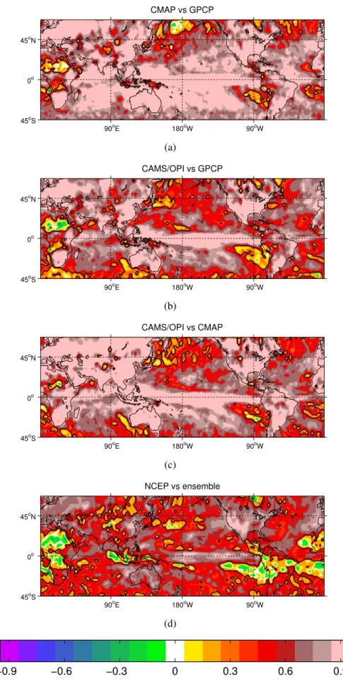
Figure 7 provides a general comparison of the three satellite rainfall products used to build the ensemble. It can be seen in a) - c) that CMAP, CAMS/OPI and GPCP agree well with each other almost everywhere in both the tropics and extratropics. This is indicated by correlation coefficients of > 0.6 almost everywhere. In particular, the three products are highly correlated (r > 0.9) over the tropical oceans, as well as over most parts of the continents. The correlations are lower over the subtropical and especially over the subpolar oceans. In these regions, DJF mean rainfall is, at the 95% confidence level, locally not even significantly correlated amongst the three rainfall products. Continental regions where the three products do not agree well are Africa, Arabia and

2 Data and methods 2.2 General rainfall analysis

90^oE 180^oW 90^oW

45^oS 0^o 45^oN

CMAP vs GPCP

(a)

90^oE 180^oW 90^oW

45^oS 0^o 45^oN

CAMS/OPI vs GPCP

(b)

90^oE 180^oW 90^oW

45^oS 0^o 45^oN

CAMS/OPI vs CMAP

(c)

90^oE 180^oW 90^oW

45^oS 0^o 45^oN

NCEP vs ensemble

(d)

r

−0.9 −0.6 −0.3 0 0.3 0.6 0.9

Figure 7:DJF winter mean local correlation coefficient between a) CMAP and GPCP, b) CAMS/OPI and GPCP, c) CAMS/OPI and CMAP, d) NCEP/NCAR and the satellite ensemble mean rainfall.

Note that NCEP/NCAR rainfall is not used to calculate the ensemble mean. Colour contouring in steps of 0.1. Black line shows the 95% confidence level of the correlation (rcrit≈ ±0.35).

Time series have been detrended.

2 Data and methods 2.2 General rainfall analysis

the south-eastern vicinities of the Atlantic and Pacific oceans. When comparing this with figure 3 a), one finds that those regions where the three satellite based rainfall products differ most strongly from each other, are regions of very weak rainfall variability. These regions are namely the Sa- hara, Arabia and the Subtropical eastern ocean basins, where maximum monthly rainfall standard deviation barely exceeds 1 mm/day. In Figure 7 d), the correlation of the ensemble mean rainfall with the NCEP rainfall is provided. Although NCEP rainfall is not included in our ensemble mean rainfall, it is striking that the correlations are overall substantial weaker than for any of the satellite based products [a) - c)]. In the regions of the Maritime Continent, Congo and South America, for example, the correlation with the satellite ensemble is mostly smaller than 0.3 and not significant.

Even in the tropical Pacific region, where the satellite products agree well with each other, corre- lation coefficients of only 0.6 - 0.8 are found. This illustrates the reason for not using DJF NCEP rainfall in our analysis.

Throughout this study, statistical significance of correlations and regressions is calculated us- ing the p-value of a test statistic (two-sided students t-test), where the Null Hypothesis is that the true Pearson correlation coefficient is zero. In all cases, the time series have been detrended. Be- fore computing the correlation coefficient, it is assumed that each year is independent of the other.

The number of degrees of freedom equals the number of winters (summers) making up the time series.

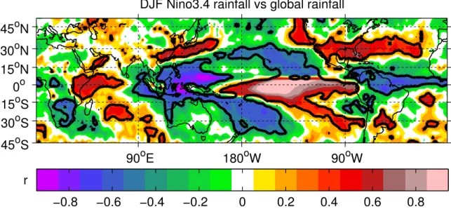
Regarding the winter time, a strong correlation between most of the time series is found, espe- cially in the Pacific sector (see Table 2). For completeness, Figure 8 shows the impact of ENSO on the local rainfall in most parts of the world. These results demonstrate the strong impact of ENSO, even in regions far away from the Nino3.4 box. In order to extract variability in rainfall which is not due to ENSO, the linear effect of the Nino3.4 rainfall signal is removed from each

Nino3.4 CP SA GU MC IO

Nino3.4 1 0.38 -0.57 0.39 -0.85 0.35

CP 0.38 1 -0.68 0.36 -0.62 n.s.

SA -0.57 -0.68 1 n.s. 0.69 n.s.

GU 0.39 0.36 n.s. 1 -0.46 n.s.

MC -0.85 -0.62 0.69 -0.46 1 -0.42

IO 0.35 n.s. n.s. n.s. -0.42 1

IND CH Sahel

IND 1 n.s. 0.56

CH n.s. 1 n.s.

Sahel 0.56 n.s. 1

Table 2: Correlation coefficients of DJF (left) and JJAS (right) rainfall time series, "n.s." means correla- tion is not significant the 95% confidence level (r_crit≈ ±0.35)

2 Data and methods 2.3 Removing the ENSO signal

90^oE 180^oW 90^oW 45^oS

30^oS 15^oS 0^o 15^oN 30^oN 45^oN

DJF Nino3.4 rainfall vs global rainfall

r

−0.8 −0.6 −0.4 −0.2 0 0.2 0.4 0.6 0.8

Figure 8:Correlation coefficient of DJF Nino3.4 rainfall with global rainfall. Colour contouring in steps of 0.1. 95% confidence interval of the correlation is indicated by the black line. Critical correlation coefficient is≈ ±0.35. Time series have been detrended.

time series. The procedure is described in the next section. In summer (JJAS), the only correlation that is significant at the 95% confidence level is found between India and Sahel (r = 0.56). This link is well known and documented in the observational and modelling climate community (see, for example, Kraus (1977), Ward (1998), Raicich et al. (2003), Zhang and Delworth (2006)) and will be picked up later.

In the JJAS analysis, there is no significant correlation found between India and Northern China.

However, in the community, this link is a topic of discussion (Sun et al., 2010, Greatbatch et al., 2013, for example) and will be further examined later.

2.3. Removing the ENSO signal

In the last section we showed that the footprint of Nino3.4 rainfall is found in most of the rainfall time series in the winter. Figure 8 provides evidence that in the winter season, interannual rainfall variability over many parts of the tropical and subtropical oceans and continents is related to the interannual variability of ENSO. A summary of rainfall patterns that are associated with ENSO is given, for example, in Ropelewski and Halpert (1987). In order to isolate the non - ENSO related rainfall signal, a regression analysis is carried out to remove the Nino3.4 rainfall signal from all the time series on the grid, such that the correlation coefficient between any rainfall time series and the Nino3.4 rainfall is zero. In other words, from each time series the part is subtracted which is linearly congruent with the Nino3.4 signal. The regression is done to the DJF and JJAS anomalies,

2 Data and methods 2.3 Removing the ENSO signal

19800 1985 1990 1995 2000 2005 2010 2

4 6 8 10 12

Nino3.4

mm/day

m= 2.27 sd= 0 m= 2.27 sd= 2.7

19800 1985 1990 1995 2000 2005 2010 2

4 6 8 10 12

SA

mm/day

m= 6.17 sd= 0.8 m= 6.17 sd= 0.98

19800 1985 1990 1995 2000 2005 2010 2

4 6 8 10 12

GU

mm/day

m= 5.45 sd= 0.55 m= 5.45 sd= 0.6

19800 1985 1990 1995 2000 2005 2010 2

4 6 8 10 12

IO

mm/day

m= 5.74 sd= 1.17 m= 5.74 sd= 1.25

19800 1985 1990 1995 2000 2005 2010 2

4 6 8 10 12

MC

mm/day

m= 8.56 sd= 0.64 m= 8.56 sd= 1.2

19800 1985 1990 1995 2000 2005 2010 2

4 6 8 10 12

CP

mm/day

m= 7.28 sd= 2.18 m= 7.28 sd= 2.36

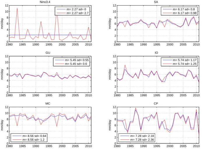
Figure 9:DJF mean rainfall estimates including (red) and excluding (blue) the Nino3.4 rainfall signal for the rainfall boxes in Table 1 and Figure 4. Note the mean stays constant.

CP SA GU MC IO

CP 1 -0.61 n.s. -0.62 n.s.

SA -0.61 1 n.s. 0.47 n.s.

GU n.s. n.s. 1 n.s. n.s.

MC -0.62 0.47 n.s. 1 n.s.

IO n.s. n.s. n.s. n.s. 1

Table 3:Correlation coefficients of DJF rainfall time series without the ENSO signal, "n.s." means correlation is not significant the 95% confidence level. The corresponding time series are shown in Figure 9.

while the original mean precipitation for each box is added back. This technique ensures that the mean rainfall at each site stays untouched, while the Nino3.4 signal gets removed. The corresponding rainfall time series are shown in Figure 9. Given the change in the standard deviations be- tween the blue and the rad curves in Fig- ure 9, it also becomes obvious that a sig- nificant fraction of variability is removed from the time series, especially for the MC

rainfall. Note the strong El Niños of 1983, 1992 and 1997 are not evident anymore in the corrected time series. However, even after removing the effect of Nino3.4 rainfall from the other time series, one can see there is still remarkable coherence over the tropical Pacific region (see Table 3), with SA rainfall being in opposite phase to CP and in phase with MC rainfall. We note that throughout

2 Data and methods 2.4 Atmospheric variables

1950 1960 1970 1980 1990 2000 2010

5 5.5 6 6.5 7 7.5 8 8.5 9

year

mm/day

All India rainfall vs ensemble mean IND (r = 0.82)

All India Rainfall GPCP

CAMS/OPI CMAP ensemble mean

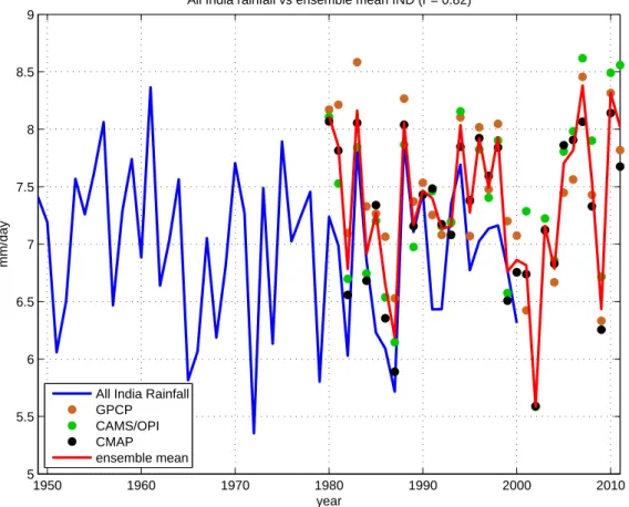
Figure 10:All India JJAS rainfall time series (blue), JJAS satellite products (dots) and JJAS ensemble mean rainfall (red). ENSO is removed. Correlation coefficient between the blue and the red curve is 0.82 in the period of overlap.

the remainder of this thesis, Nino3.4 rainfall has been systematically removed from any rainfall time series that is discussed, even for those in summer and from those which are not significantly correlated with Nino3.4 rainfall.

Figure 10 shows time series of All India rainfall together with the satellite estimates for the India box. In their overlapping time period, the satellite ensemble and All India rainfall are correlated at 0.82. Given the different spatial resolutions and inhomogeneity of the data, this is a surprisingly high value.

2.4. Atmospheric variables

We use monthly mean, gridded NCEP/NCAR data (Kalnay et al., 1996) for wind field, stream- function, geopotential height and sea level pressure. Geopotential height and wind field data are available on pressure levels on a 2.5^◦x 2.5^◦spatial grid from 1948 to present. Streamfunction is available as spectral model output (T62) from the NCEP/NCAR reanalysis, with an approximate spatial resolution of 1.875^◦and a sigma coordinate as the vertical variable.

2 Data and methods 2.5 Documented recurrent teleconnection patterns

2.5. Documented recurrent teleconnection patterns

Wallace and Gutzler (1981) find five dominant teleconnection patterns in the monthly mean winter- time northern hemisphere circulation. When analysing atmospheric teleconnections, most studies concentrate on the boreal winter, since low frequency variability is most pronounced in that season (Blackmon, 1976). In this section, we will introduce the most prominent teleconnection patterns in DJF mean data. One is the East Atlantic (EA)pattern, which is defined by three centers: one south west of the Canary Islands (25^◦N, 25^◦W) , one near the Black Sea (50^◦N, 40^◦W), and a third, oppositely-phased center west of Great Britain (55^◦N, 20^◦W). The index of the EA pattern is then given by

EA= 0.5·Z(55^◦N,20^◦W)−0.25·Z(25^◦N,25^◦W)−0.25·Z(50^◦N,40^◦E)

As in Wallace and Gutzler (1981), Z is the normalized anomalous 500hPa geopotential.

The North Atlantic Oscillation (NAO)was first described by Walker and Bliss (1932), who used normalized anomalous DJF temperature and pressure to yield:

N AO=P_{V ienna}+T_Bodö+T_Stornoway+ 0.7·P_Bermuda−PStykkisholm

−P_Ivigtut−0.7·T_Godthaab + 0.7·(T_Hatteras+TW ashington)/2

According to this, a positive NAO index goes along with a stronger than usual Icelandic low, strong westerlies along the North Atlantic and higher than usual pressure at the Azores and in the Mediterranean at about 40^◦N. Using this general feature of the traditional NAO index from Walker and Bliss (1932), many authors simply construct their NAO index based on the surface pressure difference between the Azores and The Greenland/Iceland region, in order to avoid using as much as nine different inputs (e.g. Hurrell, 1995).

At this point, one general problem becomes obvious, which was already stressed by Wallace and Gutzler (1981) and, for the special case of the NAO, by Hurrell et al. (2003). It is difficult to establish one unambiguous definition for a certain teleconnection pattern, which often complicates the direct comparison with other studies that use different analysis.

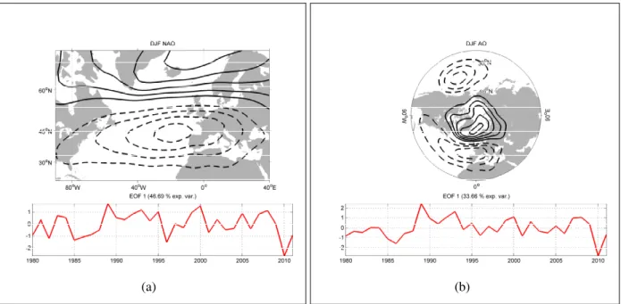
In this study, however, we compute the NAO following Hurrell et al. (2003) as the first EOF of DJF

2 Data and methods 2.5 Documented recurrent teleconnection patterns

(a) (b)

Figure 11:(a) NAO and (b) AO patterns and PC time series for the EOF-based definition of the NAO and AO. Contour interval is 8 gpm, negative values are dashed. Zero line is not plotted.

winter mean Z850 in the region 90^◦W - 40^◦E, 20^◦- 70^◦N, and the NAO index is then given by the PC series of this first EOF. This definition is rather natural, since it considers the Atlantic domain without any further assumptions about the shape of the NAO pattern. While the NAO considers the Atlantic domain of the northern hemisphere, one may also introduce the Northern Annular Mode (NAM), also called Arctic Oscillation (AO), obtained as the first EOF over the whole northern hemisphere north of 20^◦N (Hurrell et al., 2003). Both the NAO and AO patterns are shown in Figure 11. It is obvious that the NAO and AO are not independent from each other. In fact, their PC series are correlated at 0.91.

The Pacific North American (PNA) pattern consists of four equally weighted centers: One over Hawaii (20^◦N, 160^◦W), one over Alberta (55^◦N, 115^◦W), one over the North Pacific Ocean (45^◦N, 165^◦W), and one close to the Gulf region of the USA (30^◦N, 85^◦W), with the latter two centers being opposite in phase to the former two. The mathematical expression is

P N A= 0.25·[Z(20^◦N,160^◦W)−Z(45^◦N,165^◦W) +Z(55^◦N,115^◦W)−Z(30^◦N,85^◦W)]

The PNA and EA patterns are shown in Figure 1, as found by Wallace and Gutzler (1981).

Another pattern is the Scandinavia pattern, which was first discovered by Barnston and Livezey (1987) and given the nameEurasian Pattern Type 1 (EU1). It has one center over Scandinavia be- tween 60-70^◦N, 25-50^◦E, one oppositely phased center over North west China between 30-45^◦N,

2 Data and methods 2.5 Documented recurrent teleconnection patterns

(a)

(b)

(c)

Figure 12:Z500 DJF patterns for a) PNA, b) EA, c) EU1 for both periods 1949-1979 (left) and 1980- 2010 (right). The patterns are obtained by correlating the formal pattern index, as documented in this section and in Wallace and Gutzler (1981), with global northern hemisphere Z500.

Negative correlations are dashed, contour interval is 0.2, the zero line is left out. Blue asterisks indicate statistical significance at the 95% confidence level.

2 Data and methods 2.5 Documented recurrent teleconnection patterns

80-100^◦E, and one also oppositely phased center over the Mediterranean and Spain around 35 - 50

◦N, 10^◦E-20^◦W. It will be described using

EU1 = 0.5·Z(65^◦N,37.5^◦E)−0.25·Z(37.5^◦N,90^◦E)−0.25·Z(42.5^◦N,5^◦W)

Figure 12 illustrates the spatial structure of the PNA, EA and EU1 pattern for the two independent periods 1949-1979 and 1979-2010. It is important to raise the question, to what extent the telecon- nection patterns, which were described in this section, are stationary, reproducible features in the atmosphere. For example, it was shown that the centers of action of the NAO shifted towards the east in the period 1978-97 compared to the previous decades (Lu and Greatbatch, 2002, Jung et al., 2003). Wallace and Gutzler (1981) divided their available geopotential height data into two inde- pendent data sets in order to test for the reproducibility of their derived teleconnection patterns, but their data only covered 15 years. Here, we divide the available period of NCEP data into two subseries of equal length. The first covers the period 1949-1979, the second covers 1980-2010.

Analogous to Wallace and Gutzler (1981), we computed the pattern indices for the PNA, EU1 and the EA pattern using the above mathematical expressions.

From Figure 12 it can be deduced that the correlations resemble those of Wallace and Gutzler (1981) very closely, and also the significant parts of the patterns seem to be stationary, since they coincide in most locations in the analysis of both periods. Differences in the patterns are also apparent. For example, in the later period, the EA pattern is correlated with a region over North America and the influence over Scandinavia becomes less important.

The three centers used to define the EU1 pattern seem to be in a stationary relationship, but in the later period, Z500 in the Pacific region and over North America is also significantly correlated with the index. Thus, between 30^◦and 45^◦N, there appears a circumglobal chain of centers of action, illustrated by the patches of negative correlation. This is an interesting feature, because it resembles the circumglobal summer teleconnection found by Ding and Wang (2005). This pattern will be discussed more in detail in section 6. However, one should keep in mind that a signal, which is dependent on a geographic location, does not necessarily mean that the atmospheric re- sponse to any kind of geographically fixed forcing is also a stationary feature. Greatbatch et al.

(2004), for example, pointed out that the impact of ENSO on the whole European sector is not a robust feature on interdecadal timescales. In their regression analysis, the response over northern Europe even switches its sign between the periods 1958-77 and 1978-97. This should be kept in

2 Data and methods 2.6 Wave guides and Rossby wave source

mind when interpreting the results of the present study, since the regressions here only cover the satellite era.

2.6. Wave guides and Rossby wave source

Understanding the effect of Rossby wave propagation and dispersion on a rotating sphere is one key element in studies examining the atmospheric response to a certain prescribed forcing. Following the work of Sardeshmukh and Hoskins (1988), the central point is to find solutions to the vorticity equation:

∂

∂t+v· ∇

!

q=S+F (1)

whereq=ζ+fis absolute vorticity, given by the sum of relative vorticityζand planetary vorticity f. S is a source term, which is referred to as theRossby wave source (RWS). The RWS is, from a classical perspective, associated with vortex stretching, and has been expressed in earlier studies simply as −qD, where D is divergence. After decomposing the flow field into its rotational and divergent components, Sardeshmukh and Hoskins (1988) pointed out the importance of including the effect of the advection of vorticity by the divergent flow field, which is usually associated with tropical upper tropospheric divergence. Putting this together, one gets the final expression for the RWS:

S=−v_χ·∇q−qD (2)

where v_χ is the divergent wind field. It has been shown that stationary Rossby waves cannot exist in a easterly flow regime (Webster and Holton, 1982). This stresses the importance of the

90^oE 180^oW 90^oW 60^oS

30^oS 0^o 30^oN 60^oN

DJF mean RWS

RWS [ day−2]

−4

−3

−2

−1 0 1 2 3 4

Figure 13:DJF mean RWS at 200 hPa from the NCEP/NCAR reanalysis. Contour interval is 1 day⁻².

geographical location of a RWS, that is associated with a specified forcing.

Figure 13 shows DJF mean RWS for the period 1979 - 2011. The strongest RWS’s are found in the vicinity of the North African/Asian jet, as well as in the Atlantic sector and in the central Pacific sector around 30^◦N, where the corresponding jet exit re- gions are located. The Indian part of the South Asian jet reveals strongest values. In the southern hemisphere,

2 Data and methods 2.6 Wave guides and Rossby wave source

0^o 90^oE 180^oW 90^oW 60^oS

30^oS 0^o 30^oN 60^oN

Ks DJF mean

wave number

0 2 4 6 8

Figure 14:DJF meanKSat 200 hPa in units of waves circling around a latitude band. Contour interval is 2. Regions that are not coloured are regions of mean easterlies.

there are regions of positive RWS south of the continents of Australia, South America and Africa.

We note that these are regions of prevailing mean westerlies. In another study, Hoskins and Am- brizzi (1993) further analyse the characteristics of Rossby wave propagation. They find a critical zonal wave number for stationary Rossby waves in a westerly flowU¯, which is

K_S = β^∗ U¯

!1/2

(3) where

β^∗ =β− ∂²U¯

∂y² (4)

is the meridional gradient of absolute vorticity. Hoskins and Ambrizzi (1993) further argue that Rossby waves will be refracted meridionally towards regions of larger K_S. Figure 14 reveals the existence of zonally aligned regions of maximum values ofK_S, which are in good agreement with the location of the midlatitude jet streams. Their amplitude and location also agrees well with Figure 3 c) in Hoskins and Ambrizzi (1993). One may interpret these structures as Rossby wave guides and we note that an anomalous RWS, which is located within the vicinity of such a wave guide, can be effective in generating a global scale teleconnection due to Rossby wave propagation.

As pointed out in Sardeshmukh and Hoskins (1988), diabatic heating in the equatorial region can induce anomalous RWS’s in the subtropical westerlies, where it is effective in generating planetary wave motion. We will stress this theoretical concept in our analysis of local rainfall which initiates an anomalous RWS in regions where RWS driving is very effective.

3 Tropical Pacific teleconnections

3. Tropical Pacific teleconnections

3.1. ENSO teleconnections

0^o 90^oE 180^oW 90^oW 60^oS

30^oS 0^o 30^oN 60^oN

Nino3.4 rainfall vs Z200

gpm

−50

−40

−30

−20

−10 0 10 20 30 40 50

(a)

0^o 90^oE 180^oW 90^oW 60^oS

30^oS 0^o 30^oN 60^oN

Nino3.4 rainfall vs Ψ at σ=0.21

Ψ[m2/day]

−80

−60

−40

−20 0 20 40 60 80

(b)

Nino3.4 rainfall vs Z850

0^o 90^oE 180^oW 90^oW 60^oS

30^oS 0^o 30^oN 60^oN

gpm

−30

−20

−10 0 10 20 30

(c)

0^o 90^oE 180^oW 90^oW 60^oS

30^oS 0^o 30^oN 60^oN

Nino3.4 rainfall vs Ψ at σ=0.85

Ψ[m2/day]

−50 0 50

(d)

Figure 15:Maps using DJF mean data of (a) geopotential height at 200 hPa and (c) 850 hPa, and stream- function atσlevels (b) 0.21 and (d) 0.85 regressed onto Nino3.4 rainfall. The pattern corre- sponds to one standard deviation of the detrended rainfall time series. Contour interval is (a) 10 gpm, (b) 20 m²/day, (c) 6 gpm, (d) 10 m²/day. Negative (positive) values are highlighted blue (red), bold contours mark significance of the regression slope at the 95% confidence level. Corresponding rainfall time series is shown in Figure 9.

Anomalous heating in the eastern tropical Pacific has been shown in many studies to initiate global scale anomalies in the atmospheric circulation. For example, Trenberth et al. (1998) describe how anomalous heating associated with ENSO perturbs the atmosphere, and how the perturbation spreads towards the extratropics, including changes in the Hadley cell circulation in the meridional- vertical plane, as well as upper level divergence and lower level convergence of anomalous zonal winds in the heating region. We provide evidence for the existence of preferred teleconnection pat- terns for ENSO related diabatic heating using the 1980-2011 satellite ensemble mean rainfall as a

3 Tropical Pacific teleconnections 3.1 ENSO teleconnections

5 m/s

180^oW 120^oW 60^oW 0^o 60^oE 120^oE 180^oW 30^oS

15^oS 0^o 15^oN 30^oN

wind 200 hPa

(a)

3 m/s

180^oW 120^oW 60^oW 0^o 60^oE 120^oE 180^oW 30^oS

15^oS 0^o 15^oN 30^oN

wind 850 hPa

(b)

Figure 16:DJF Nino3.4 rainfall regressed on wind in (a) 200 hPa and (b) 850h Pa, grey shading marks significance of the regression slope at the 95%confidence level. The pattern corresponds to one standard deviation of the detrended Nino3.4 rainfall series.

representation of diabatic heating. Figure 15 shows atmospheric circulation patterns that are asso- ciated with Nino3.4 rainfall. At 200 hPa, a positive circumglobal Z200 anomaly can be identified along the equator, indicating anomalous high geopotential height in the troposphere, associated with the warming of the tropical band during an El Niño.

Another main result, which seems to be in general agreement amongst the tropospheric regres- sion maps in this study, is that the atmospheric response has a strong barotropic component in the extratropics, while the responses seem to be rather baroclinic in the tropics. Z500 regressions were performed as well, but given their strong similarities to the Z200 regression maps, they are not shown. Nino3.4 rainfall is associated with significant strengthening of the Aleutian low, and anomalous positive Z200 over Hudson Bay. This is well known to be part of the PNA pattern (see section 2.6), although the positive anomaly over Hawaii is only apparent in Z200, while the negative anomaly center over the Gulf of Mexico is more clearly to see in the Z850 regression.

The correlation coefficient of Nino3.4 rainfall and the PNA pattern index, as defined in section 2.6, is 0.63. There is also a teleconnection to the Southern hemisphere, which involves a structure somewhat similar to the Pacific South American (PSA) pattern (Mo and Peagle, 2001), that is,

3 Tropical Pacific teleconnections 3.1 ENSO teleconnections

anomalous high pressure between southern South America and the Ross Sea and anomalous low pressure at the same longitudinal position around 45^◦S. The amplitudes and spatial structure of both PNA and PSA patterns in the regressions show a remarkable degree of equatorial symme- try. Trenberth et al. (1998) argue, that the PNA pattern might be largely the response to ENSO related tropical heating in the Pacific, although a fraction of variability of the PNA pattern dy- namics is due to internal atmospheric variability. They further assess the PSA pattern to be the Southern hemisphere counterpart of PNA pattern, or even the "footprint" of ENSO in the South- ern hemisphere. We present regressions on streamfunction shown in Figure 15 b) and d), because close to the equator, the geostrophic approximation breaks down, and geopotential height may not be an appropriate indicator for the tropospheric flow. However, we wish to also highlight the tropospheric response close to the equator. At upper tropospheric levels (σ=0.21), there are two equator-symmetric anticyclonic anomalies found north and south of the equator west of the asso- ciated Nino3.4 rainfall box. This is consistent with theory (Gill, 1980). Spreading north-eastwards and south-eastwards off the equator, they closely follow the teleconnection structures in the geopo- tential height. The process for exciting such far-reaching teleconnections is explained in Trenberth et al. (1998): Above the forcing region, there is meridional outflow at upper tropospheric levels, which leads to upper tropospheric convergence in the subtropics, and thus, generation of anoma- lous high pressure and enhanced anticyclonicity there. Trenberth et al. (1998) further argue that this anomalous divergent wind can act as Rossby wave source in order to initiate the Rossby wave response that carries the information about the tropical disturbances towards higher latitudes, fi- nally setting the well documented teleconnection patterns. However, the existence of those two upper-tropospheric anticyclones west to the region of equatorial heating is a very fundamental fea- ture of the atmospheric response in all of our regressions that are associated withtropicalrainfall, although weaker in most other cases. The tropical regression patterns presented in this section are in agreement with what is expected from linear theory (Gill, 1980), indicating that the nature of the response in the tropics is mainly governed by linear dynamics.

Regarding the patterns in Figure 15, we finally point out two more aspects. First, the pattern in Figure 15 a) and b) projects on a negative phase of the Southern Annular Mode (SAM), such that an impact on Antarctic climate and the Southern Ocean is possible (Ding et al., 2015). Second, the significant negative anomaly over Cape Hatteras in Figure 15 c) implies a remote impact on climate over this part of the Gulf Stream. In fact, DJF rainfall in our Gulf Stream box is correlated with the Nino3.4 rainfall at 0.39, which is significant at the 95% confidence level (see Table 2).