Human Activity Recognition from Video: modeling, feature selection and classification architecture

Human Activity Recognition from Video: modeling, feature selection and classification architecture

Pedro Canotilho Ribeiro & Jos´e Santos-Victor

Instituto Superior T´ecnico

Instituto de Sistemas e Rob´otica Lisboa, Portugal

{pribeiro, jasv}@isr.ist.utl.pt

Abstract

In this paper, we address the problem of recognizing human activities, such as{Active, Inactive, Walking, Running, Fighting}from video sequences, with a particular emphasis on the problems of feature selection, data modeling and classifier structure.

The need for such systems is increasing everyday, with the number of (hundreds or thousands) of surveillance cameras deployed in public spaces. This massive number of cameras calls for systems able to detect, categorize and recognize human activity, requesting human attention only when necessary.

Our work is focused on three fundamental issues: (i) the design of a classifier and data modeling for activity recognition; (ii) how to perform feature selection and (iii) how to define the structure of a classifier.

We use of a Bayesian classifier, and model the likelihood functions as Gaussian mixtures, adequate to cope with complex data distributions, that are learned automatically. As for feature selection, we propose several (suboptimal) methods to evaluate the recognition rate achieved with different feature combina- tions, with the Bayesian classifier. Finally, we investigate the use of hierarchical classifiers (including the possibility of automatic generation).

Our results were based on nearly 16,000 images of five activities and we achieved an error rate as low as 1.5%. These experiments clearly demonstrate the importance of powerful methodologies for data modeling and how intertwined feature selection, classifier design and the structure of the classifier are.

1 Introduction

In this paper, we address the problem of recognizing human activities from video sequences, with a particular emphasis on feature selection, data modeling and classifier structure.

Recently, human motion analysis has become one of the most active research areas in computer vision. This is due to promising applications in areas such as visual surveillance, human performance analysis, computer-human interfaces (robotic interaction with humans), content-based image retrieval/storage and virtual reality.

Human movements can be considered at different levels of (temporal) detail: the analysis of the movement of body parts, single person activities and, over increasing temporal windows, large-scale interactions. As a consequence of the application, systems must deal with different activities and temporal integration times.

Most systems that perform human motion analysis address general common tasks, such as: person detection &

tracking, activity classification, behavior interpretation and also person identification. Obviously, although some of these tasks can be considered independently, they must be solved in a common framework, where information can be communicated and exchanged between the different system modules.

As the detection and tracking systems have progressed significantly in the past few years, [4, 12, 5], human motion and behavior interpretation have naturally become the following step. In a surveillance scenario, tracking is the very first step and behavior recognition the final goal. The task of activity recognition can be viewed as a bridge between the pixel measurements, given by the tracker, and a more abstract behavior description.

In this paper, we focus on this intermediate level, that is essential to achieve the desired final large-scale interpre- tation. The need for such systems is increasing everyday with the number of surveillance cameras deployed in public spaces. Needless to say, the “traditional” job of the security operator, monitoring several video streams for extended periods of time, becomes impossible, as the number of cameras grows exponentially. Instead, we need systems able to detect, categorize and recognize human activity, calling for human attention only when necessary.

Generally, human action interpretation can be divided in three [1] major approaches. Generic model recovery tries to fit a 3D model to the person pose [12], and is usually strongly dependent on a accurate 3D feature extraction.

∗This work has been partially supported by EU project CAVIAR(IST-2001-37540) and by the portuguese Fundac¸˜ao para a Ciˆencia e Tecnologia, Programa Operacional Sociedade de Informac¸˜ao (POSI), in the framework of the III Quadro Comunit´ario de Apoio.

HAREM 2005 - International Workshop on Human Activity Recognition and Modelling, Oxford, UK, September 2005

Appearance-based models, are based on the extraction of a 2D shape model, directly from the images, to be classified (or matched) against a trained one [4, 2, 10, 1]. Motion-based models do not rely on static models of the person, but on people motion characteristics [3, 1, 10].

In [5] human actions are represented by stochastic finite automaton of event states, that recognize human interac- tions like conversing or taking objects away, from trajectory and shape characteristics. Shape analysis and tracking can also be used to construct models of people appearance, ordering the body parts on the silhouette boundary, in order to monitoring their activity [4]. In this case the work is constrained to lateral view of the people.

Bobick and davis work [1] used Motion Energy and Motion History Images (MEI and MHI) to classify “aerobic”- type exercises. In [2], these same images are used determine the shortest video exposure needed for low-latency recognition, using a reliable-inference framework to differentiate between walking, running and standing activities.

The work of Rosales [10] also uses the invariant 7-Hu moments of MEI and MHI to estimate Gaussian Mixtures models of Walking, Running, Roller Blading and Biking activities.

Efros et al [3] compute optical flow measurements in a spatio-temporal volume to recognize human activities in a nearest-neighbor framework. In this work, Ballet, Tennis and Football sequences are used to evaluate the proposed approach. In [8] several activities, like Walking, Running, Marching and skipping were recognized, although in a constrained scene, using motion filtered images and space reduction technicques.

The CAVIAR [13] sequences are used in [7] to recognize a the set of activities, scenarios and roles. The approach generates a list of features and automatically chooses the smallest set, that accurately identifies the desired class.

However, the results reported use the same sequences (different images) for testing and training. Therefore, it is not clear how the recognition rates would generalize with different sequences.

Although there are many works that can identify interesting activities, many of the applications are scene depen- dent, i.e. frequently tailored to one specific training scenario. This is the case of [7], because of the use of features like the target position and orientation. Even though this process can model scene depth variations (needing a large set of training examples), it needs to be repeated for each new scenario.

In our work, we try to overcome some of the difficulties discussed before and address three fundamental issues for an activity recognition system: (i) the design of a classifier; (ii) how to perform feature selection and (iii) how to define the structure of a classifier.

We assume that a tracking system computes the subject spatial and temporal grouping (i.e. the person detected pixels over time). We further assume that the tracker measurements are corrected using the image-to-ground plane projective transformation, thus achieving scene (viewpoint) invariance [9].

As for the design of the classifier, we propose the use of a Bayesian classifier, where the likelihood functions are modeled as Gaussian mixtures, estimated from data. This modeling approach proves to be adequate for the complexity of data distribution we face in this domain.

Regarding the crucial aspect of feature selection, we start with a rich set of 29 features, that describe the subjects global motion, as well as local motion within the region of interest. We propose several (suboptimal) methods for feature selection, to evaluate the recognition rate with the Bayesian classifier. All results are obtained with real images (ground truth available), with different training and test sequences (not just different images, but sequences).

To improve the results, we investigated the use of hierarchical classifiers by grouping the activities to recognize.

We show that a hierarchical classifier, with automatic feature selection, achieves an error rate as low as 1.5%. Finally, we briefly address the problem of automatically generating the structure of the hierarchical classifier.

Our experiments clearly show the importance of data modeling methodologies and how intertwined feature selec- tion, classifier design and the structure of the classifier are. The experiments conducted and the encouraging results achieved have been obtained with nearly 16,000 images, with ground truth available.

Section 2 describes the activities to recognize within this work, as well as the large set of features we will analyze and evaluate. Section 3 is devoted to the description of the Bayesian Classifier as well as the feature selection methods.

Results with a single layer classifier are presented. Section 4 addresses the problem of hierarchical classification and proposes several classifiers, with an average error rate as low as 1.5%. Finally, in Section 5 we draw some conclusions and establish future directions of work.

2 Low level activities and features

We have concentrated on low-level, short term human activities, as those studied in the context of the CAVIAR project [13]. We will explore the availability of a large data set of video sequences and manually classified activities, in a total of about 16,000 images with ground truth data. The activities (classes) considered can be detected from a relatively short video sequence (a few seconds) and are described in Table 1.

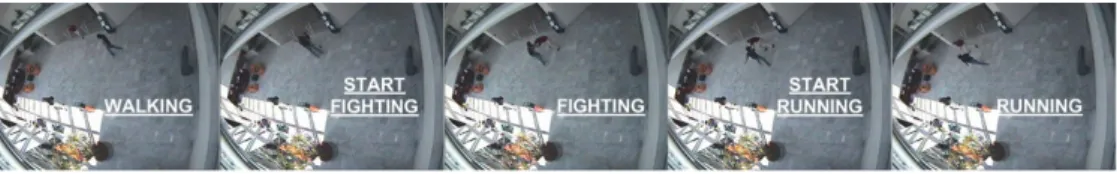
From this basic set of activities, more complex activities can be formed, over larger intervals of time. In those cases, the use of contextual information can help distinguishing activities that would otherwise be ambiguous. Figure 1 shows images acquired in one test scenario corresponding to the referred activities.

We now have to define a number of low-level features, that can be extracted from short video sequences, for activity recognition. Of course, one can only assess the quality of a feature once a classifier (or a metric) is designed for a specific problem. In other words, feature definition and classification are intertwined problems.

id # Frames Activity Description

1 3,211 Inactive a static person/object

2 1,974 Active person making movements but without translating in the image.

3 9,831 Walking there are movements and overall image translation 4 297 Running as in walking but with larger translation.

5 594 Fighting large quantities of movement with few translation.

Table 1: Low-level activities and data distribution.

Figure 1: Example images and observed activities in one of the CAVIAR test scenarios.

We start by defining a comprehensive set of features that, intuitively, may distinguish the different activities. Then, we assess the quality of those features by analyzing the error rate of our classifiers, against the CAVIAR data-sets.

We assume the existence of a tracking system, able to identify moving blobs in the scene (e.g. though background subtraction, with adaptive background models [4]) and provide information regarding the position of the target over time. When tracking a person across the camera field of view, size, appearance and speed are influenced by perspective.

This makes the classification process more difficult, since the observed measurements depend both on the ongoing activity and on the viewing geometry. To achieve viewpoint invariance, all image measurements are back-projected onto the ground plane, using the projective planar transformation between the image and scene ground planes. Figure 2 illustrates the observed (perspectively distorted) image and an orthographic view of the ground plane obtained with the estimated homography.

Figure 2: Original (left) and resulting transformed (right) images of the INRIA - Caviar scenario. Perspective distortion is removed by mapping the ground plane using the estimated homography.

From this point onwards we will assume that the tracker uses the ground-image planes homography, to express the position estimates of the bounding box, directly in the ground floor coordinates. The first sub-set of features have the goal of representing the target global position over time. The second sub-set of features describes the internal motion of the blob.

2.1 Features

We consider two reasonably large sets of features, each organized in several subgroups. The first subset of features code the instantaneous position and velocity of the tracked subject. The target velocity,~v(t), and speed, v(t), are obtained through differentiation of the instantaneous position estimate (first sub-group) . Since the target inter-frame displacements can be very small, the temporal derivative can be quite noisy. Hence, we introduce different ways of averaging the velocity and speed estimates over an interval of T frames (second sub-group). The average velocity can be estimated in 4 different processes: (i) simple averaging; (ii) combining velocity estimates over different time inter- vals; (iii) least squares fit to a constant velocity (linear) model or (iv) least squares estimate of a constant acceleration (quadratic) model.

One interesting potential feature is the ratio between the average speed and the norm of the average velocity. It describes how irregular the motion actually is, approaching 1 if the target always moves in the same direction along a straight line and tending to 0 if it moves irregularly in various directions, or returns to the initial position.

The third sub-group of features aim at coding the temporal energy or activity. It basically consists in taking second order moments of the speed or velocity, either centered or non centered. For the matrices corresponding to the

second order moments of the target velocity we further compute the trace and the ratio of the two eigenvalues. These parameters describe the total energy and the dominant directions with respect to the velocity energy distribution.

Table 2 shows the features described. Only those features with a corresponding index in the first column of the table will be evaluated as features in the system. The others correspond to auxiliary computations.

# NAME DEFINITION

Instantaneous - position ~p(t) = (X(t),Y(t))

- velocity ~v(t) =^d~_dt^p= (vx(t),vy(t))'(X(t)−X(t−1),Y(t)−Y(t−1))

1 speed v(t) =k~v(t)k=

q

v²_x(t) +v²_y(t)

Time averaged over T frames 2 mean speed v¯T(t) =_T¹∑^ti=t−T+1v(i)

- mean velocity norm ||v~¯_T(t)|| ⇒Use one of 4 different methods:

3 - averaging vectors ||v~¯T(t)||₁=||1 T

t−1

∑

i=t−T

~p(t)−~p(i) t−i ||

4 - mean vector ||v~¯T(t)||2=||1 T

∑

~v(i) =~p(t)−~p(t−T+1)

T ||

5 - linear fitting ||v~¯T(t)||3=Linear Least Squares Fitting 6 - quadratic fitting ||v~¯_T(t)||₄=Quadratic Least Squares Fitting 7..10 speed/velocity ratio R_v~T(t)_i= v¯_T(t)

||v~¯T(t)||i

,i=1,2,3,4

Temporal energy/2nd order moments 11 speed σ_v²(t)₁=_T−1¹ ∑^ti=t−T+1v²(i)

12 speed (centered) σ_v²(t)₂= 1 T−1

∑

(v(i)−v¯T(t))² - velocity Σ~v(t)1=_T−1¹ ∑^ti=t−T+1~v(i)~v(i)^T - velocity (centered) Σ~v(t)2= 1

T−1

∑

~v(i)−v~¯T(t)

~v(i)−v~¯T(t)T

13,14 trace tr_Σ~v(t)i=trace(Σ~v(t)i),i=1,2.

15,16 eigenvalues ratio R_Σ~v(t)_i= ^λmin

λmax(Σ~v(t)_i),i=1,2.

Table 2: Features derived from the target global position provided by a tracker. The features are organized in 3 groups:

(i) instantaneous measurements, (ii) average speed/velocity based features and (iii) second order moments/energy- related indicators.

The second subset of features are based on estimates of the optic flow or instantaneous pixel motion inside the bounding box, as described in Table 3. We consider that the motion inside each tracked blob can be as important for activity recognition, if not more, as the overall trajectory of the bounding box.

Again, these features are divided in different sub-groups. After computing the optic flow in the target region, we compute the mean flow. As an option, the mean flow can be centered (subtracted from) with the average blob velocity.

In this way, the resulting flow corresponds to the relative motion inside the blob. We also compute the norm of the (spatially) averaged flow.

The next subgroup of features takes second order (spatial) moments of the flow or its norm (centered or non- centered). Also, the ratio of the eigenvalues of the second-order matrix is taken as indicator of the directionality of the overall energy. The following subgroup of features introduces temporal averaging over T frames, namely of the mean flow and the motion energy. Finally, the last subgroup consists in (temporal) second-order moments of the flow and the ratio of the eigenvalues, taken as an indicator of the directionality of the motion. Again, only those rows in the table that have an index in the first column correspond to features to be evaluated. All the others correspond to auxiliary computations.

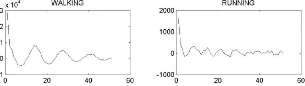
We have seen that some of the presented feature correspond to the average of instantaneous measurements, taken over T frames. Figure 3 shows the autocorrelation of the instantaneous speed for the {Running} and {Walking}

activities. It shows the “periodic” nature of the processed signal and can be used to determine a meaningful value for T . Based on this type of curves we have used T =25 frames in most of our experiments.

In the next section we will address the problem of finding out the most promising features - amongst the 29 features described - for the purpose of recognizing the human activities of Active, Inactive, Walking, Running or Fighting.

# NAME DEFINITION

Reference set of pixels - target pixels P(t) ={(x,y)∈R²|(x,y)∈target(t)}

Instantaneous - optical flow ~F(t,x,y) = (fx(t,x,y),fy(t,x,y)),(x,y)∈P(t)

- mean flow ~F¯(t)₁= _N¹∑(x,y)∈P(t)~F(t,x,y) - mean flow (centered) ~F¯(t)₂=~F(t)¯ ₁−~v(t)

- flow norm f(t,x,y)₁=k~F(t,x,y)k=q

f_x²(t,x,y) +f_y²(t,x,y),(x,y)∈P(t) - flow norm (centered) f(t,x,y)₂=k~F(t,x,y)−v~¯Tk

Spatial energy/2nd order moments 17,18 motion energy f¯(t)i= _N(t)¹ ∑(x,y)∈P(t)f²(t,x,y)i,i=1,2.

- flow covariance Σ~F(t)₁=_N(t)¹ ∑(x,y)∈P(t)~F(t,x,y)~F^T(t,x,y)

- flow covariance (centered) Σ~F(t)₂=_N(t)¹ ∑(x,y)∈P(t)(~F(t,x,y)−~F(t)¯ ₁)(~F(t,x,y)−~F¯(t)₁)^T 19,20 eigenvalues ratio R_Σ~

F(t) =^λmin

λmax(Σ~F(t)i),i=1,2.

Time averaged over T frames - mean flow ~F¯(t)_i+2=~F(t)¯ _i−¹_T∑^tj=t−T+1~F(¯ j)_i,i=1,2.

21 motion energy f¯T(t) =_T¹∑^ti=t−T+1f(i)¯ ₁

Temporal energy/2nd order moments - mean flow Σ~F¯(t)i=_T¹∑^tj=t−T+1~F(¯ j)i~F¯(j)^T_i,i=1,2,3,4.

22..25 trace tr_Σ~¯

F(t)i=trace(Σ~F¯(t)i),i=1,2,3,4.

25..29 eigenvalues ratio R_Σ~¯

F(t)i= ^λmin

λmax(Σ~F¯(t)i),i=1,2,3,4.

Table 3: Features derived from the detected target optical flow. The features are organized in 4 sub-groups: (i) in- stantaneous measurements, (ii) spatial 2nd-order moments, (iii) temporal averaged quantities and (iv) temporal second order moments/energy-related indicators.

Figure 3: Speed autocorrelation over time for the walking and running activities.

3 Feature Selection and Recognition

Having defined the activities to recognize and the list of potentially interesting features, we will now proceed to select which features prove most useful for activity recognition. The optimal solution to this problem calls for the exhaus- tive search amongst all possible feature combinations, given a classification metric. Since such approach becomes impractical, once the number of features increases, we explore suboptimal feature selection strategies for recognizing the proposed activities. In the following subsection, we present the classifier that will be used, when evaluating the discriminating power of the various feature sub-sets.

3.1 The recognition strategy

To assess the quality of the features, we have designed a Bayesian classifier that we describe hereafter. Let F(t)denote the feature vector observed at time t. The size of F(t)depends on the number of the feature components selected from the global set described in Section 2. Given a set of activitiesAj, j=1..n, the posterior probability of a certain activity taking place can be computed using Bayes rule as:

P(Aj|F(t)) =p(F(t)|Aj)P(Aj) p(F(t))

where p(F(t)|Aj)is the likelihood of activityAj, P(Aj)is the prior probability of the same activity and p(F(t))is the probability of observing F(t), irrespective of the underlying activity.

To build the Bayesian classifer, we must estimate the likelihood function of the features, given each class. The choice of the method to adopt depends on the complexity of the data distribution and dimension of the feature space.

As a consequence of the complex feature distribution, we have modeled the data as Gaussian mixtures. This model can approximate arbitrarily complex distributions, when the number of Gaussians increases. The likelihood function is thus approximated by:

p(F(t)|Ak)≈

∑

πjN (µ_j,σ_j), (1)

whereN (µ_j,σ_j)denotes a Normal distribution andπjrepresents the weight of that Gaussian in the mixture, for each listed activity,Ak. To guarantee that p(F(t)|Ak)is a proper probability distribution, we need to have∑^N_j=1πj=1 and allπj≥0.

The unknown parameters of the mixture, (µ_j,σj,πj) were estimated with the Expectation-Maximization algorithm [11]. We allow the number of Gaussians to vary by eliminating terms when they are too “similar”. In [11], a measure designated by kurtosis is used to measure how close a distribution is to a Gaussian. It is used to split the distribution if it is too different from a Gaussian. Similarly, it can be used as a closeness metric to merge distributions, if this distance becomes too small.

With this procedure, we can estimate the likelihood function without imposing any (global parametric) structure for the underlying distribution. In addition, the number of Gaussians required to model the data is an indication of how complex the data are.

For simplicity, we consider independence between the observations in different time instants. Thus, the inclusion of features extracted in a temporal window, Tc, is modeled by the product of the probabilities. The (naive) Bayes rule becomes:

P(Aj|F(t),F(t−1), ...,F(t−T_c)) =∏^T_i=0^c p(F(t−i)|Aj)P(Aj)

p(F(t)) . (2)

Having estimated the likelihood functions, and integrated the measurements over time, the Maximum a Posteriori (MAP) estimate of the observed activity is given by:

AˆMAP(t) =arg max

Aj

P(Aj|F(t−T_c, ...,t)) (3)

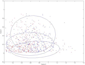
Figure 4 shows the phase-space of two features for one given activity, illustrating the complexity of data distribu- tion and the need for powerful modeling techniques. As desired, the mixture of Gaussians seems to be able to model the likelihood function.

Figure 4: Phase plot of features 9 and 21. The ellipses represent the Gaussian modes of the mixture, estimated using EM. Blue dots correspond to the training set and red dots to the test set.

3.2 Selecting promising features

We have proposed a Bayesian classifier that takes a feature vector as the input (actually, a collection of feature vectors over time) and generates a decision, regarding the observed activity.

We now have to decide upon which features to use, from the set described in Section 2. The reason for selecting a subset of those features, instead of using them all, has to do with the ability to model the likelihood function. The higher the dimension of the feature space, the more difficult it becomes to model the data distribution. In addition, learning feature distribution in a high dimensional space requires large amounts of data, which are not always available.

We evaluate the performance of the feature set using the proposed classifier. To be exhaustive, we would need to consider all possible combinations of 1 feature, 2-features, 3-features, etc. For M features (29, in our case), this would require running the classifer (and learning the likelihood functions) a large number of times:

#trials=C₁^M+C^M₂ +C₃^M+...+C_M^M

where C^M_i denotes the number of combinations of i features chosen amongst the possible total number of M features.

Needless to say, this number becomes extremely large, even for a few tens of features. Here, we follow several suboptimal strategies, to select a given number of features from the original set.

The first Brute-Search approach is the most straightforward and computationally expensive. The best Nf features are obtained by trying all possible combinations of N_f features, requiring the evaluation of C^M_N

f feature-tuples.

The second method, that we call Lite-Search, coincides with the previous method, if we just look for the best feature. If two features are needed, we then use the best individual feature and search for the feature, amongst all others, to form the best possible pair with the first one. It would then require evaluating M features individually, plus M−1 additional runs to find the “best” pair. For three features, we use the best pair and search amongst the remaining M−2 features for the best triplet, with a cost of M+ (M−1) + (M−2)runs.

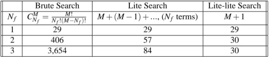
The third method, called the Lite-lite Search, aims to reduce the computational cost even further. We first rank the features individually. If we want to use two features, we rely on the best two (isolated) features and run the modeling step once more to learn the likelihood functions. Table 4 summarizes the cost of these different methods, providing numeric examples for our case of M=29.

Brute Search Lite Search Lite-lite Search

N_f C_N^M

f =_N ^M!

f!(M−N_f)! M+ (M−1) +..., (N_f terms) M+1

1 29 29 29

2 406 57 30

3 3,654 84 30

Table 4: Comparison of the search complexity, in terms of the number of runs of the classifier and modeling the likelihood function, of the used feature search methods, for our case with M=29 features.

The final method the well know Relief algorithm [6] that creates a weight vector over all features to quantify their

“quality”. This vector is updated for each of the data points presented, according to:

w_i=w_i+ (x_i−nearmiss(x)_i)²−(x_i−nearhit(x)_i)²,

where wirepresents the weight vector, xithe i^thfeature for data point x, nearmiss(x)and nearhit(x)denote the nearest point to x from the same and different class, respectively. The Relief algorithm gives larger weights to features that result in compact class clusters, while keeping the largest possible distance to the nearest class. Possible problems may arise when the data distribution does not lead to the formation of compact clusters. When all classes are “close”

to each other, evaluating only the distance to the nearest one does not necessarily guarantee quality of the feature.

In spite of this limitation, the Relief algorithm is very efficient. On a Pentium IV machine, 2.8MHz, 512Mb Ram, Relief takes about one minute of computation time, in a non-optimized MatLab implementation. Instead, the Brute- Search method takes about 24 hours to find the best triplet of features. Table 5 show the results obtained using these different feature search criteria and for 1, 2 or 3 features.

Brute Search Lite Search Lite-lite Search RELIEF

# Features Feat. R. rate Feat. R. rate Feat. R. rate Feat. R. rate

1 7 83,9% 7 83,9% 7 83,9% 14 46,8%

2 9 18 93,5% 7 25 89,8% 7 18 89,6% 14 18 59,2%

3 3 9 20 94% 7 19 25 92,1% 7 18 23 86,7% 14 18 23 57,1%

Table 5: Comparison of the recognition rate with different methods for feature selection.

From this table, we can see that the best results are obtained with the “Brute-Search” approach, as expected. With one feature only, we achieve a classification error of 16.1%, while using three features causes the error to drop down to 6%. The performance of the “Lite-Search” method is slightly inferior at a much lower search cost. Finally, the

“Lite-lite-Search” does not lead to competitive results. Similarly, the performance of the RELIEF algorithm is clearly

Class Inactive Active Walking Running Fighting Total BB

Inactive 95,2 4,8 0 0 0 1525

Active 5,8 84,7 0 0 9,5 877

Walking 0 0,2 98,1 0,8 0,9 4830

Running 0 0 0 100 0 111

Fighting 0 2,7 5,3 0 92,0 263

Table 6: Confusion matrix for the five activities and using the “best” feature triplet: F₁=9, F₂=15, F₃=22. The rightmost column indicates the total number of processed bounding boxes (targets).

behind some of other methods, probably due to the poor modeling of complex data distributions. Finally, Table 6 shows the confusion matrix corresponding to the best classifier using the best triplet of features.

We have proposed a Bayesian classifier for human activity recognition where the likelihood function was modeled as a mixture of Gaussians and estimated using the EM algorithm. Then, we have used this classifier to evaluate different feature sub-sets, using four distinct methods with different computational cost. The use of three features allowed us to recognize the observed activities with an error as low as 6%. In the following section we will see how to further reduce the error rate by using alternative architectures for the classifier.

4 Classifier Structure

We have seen the impact of feature selection on the recognition rates and on the complexity of data modeling. To improve the classification rate even further, we will change the structure of the classifier. One of the limitations of the previous classifier was that all classes had to be considered simultaneously. If a certain feature is good for two classes and another feature proves successful for two other classes, both of them will be included in the selection set. As a consequence, we will have to model the joint likelihood of those features, as opposed to modeling them separately.

Here, we will follow a different approach. We will group activities in subsets and perform classification in a hierarchical manner. Each classifier will have to deal with a smaller number of classes. In addition, we can use different features for different classifiers/classes, instead of having the same feature set for all classes.

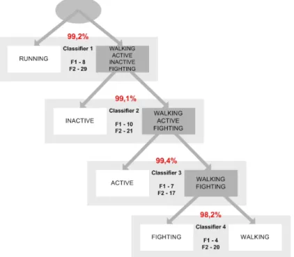
Figure 5 shows one binary hierarchical classifier. The problem of recognizing the 5 different human activities is broken down into 4 distinct classification problems, each producing a binary decision.

Figure 5: Binary tree classification with error percentage and best features selected for each classifier. The classifica- tion error is as low as 1.5%!

The first classifier distinguishes between two meta-classes:{Active, Inactive}versus{Walking, Running, Fight- ing}, using a set of features selected with the procedures described in the previous section. Then, other classifiers will try to distinguish{Active}versus{Inactive}, and so forth. We now have the flexibility to specialize the features for each subset of classes and to use different number of features for different layers of the hierarchical classifier.

Table 7 shows the recognition rate obtained with this hierarchical classifier using one, two or three features selected as described previously. The 6% error rate of the single layer classifier was reduced to 1.5%, using three features in all classifiers except for classifier 2 (see Figure 5).

Brute Search Lite Search Lite-lite Search RELIEF

# Feat. Class. Feat. Reco. rate Feat. Reco. rate Feat. Reco. rate Feat. Reco. rate

1 18 97,6% 18 97,6% 18 97,6% 14 89,2%

1 2 17 95,5% 91,4% 17 95,5% 91,4% 17 95,5% 91,4% 18 92,1% 72,3%

3 5 94% 5 94% 5 94% 23 86,7%

4 7 98,1% 7 98,1% 7 98,1% 11 85,5%

1 7 18 97,3% 18 7 97,3% 18 7 97,3% 14 23 89,8%

2 2 1 17 99,3% 95% 17 1 99,3% 94,2% 17 1 99,3% 90,3% 18 17 91,2% 69,7%

3 3 19 96,9% 5 19 95,5% 5 26 90,7% 23 18 92,8%

4 6 7 99,6% 7 6 99,6% 7 2 97,1% 11 18 69,3%

1 15 9 17 99,5% 18 7 16 98,9% 18 7 23 97,5% 14 23 25 89,8%

3 2 11 3 6 89% 94,4% 17 1 11 64,7% 73% 17 1 18 56,7% 71,8% 18 17 14 67,6% 46,3%

3 10 18 21 98,8% 5 19 18 80,9% 5 26 23 87,1% 23 18 14 61,2%

4 7 23 24 100% 7 6 2 99,3% 7 2 25 98.5% 11 18 23 86,9%

Table 7: Comparison of recognition rates obtained for the hierarchical classifier using different methods for feature selection. Error rates are presented for each individual classifier and the overall score for the hierarchical classifier.

4.1 Discussion

The hierarchical classification strategy led to significant improvements over our previous results. However, the struc- ture of the classifier, i.e. how the different classes were arranged in meta-classes, was done manually, based on our intuition as to how they should be combined together. Even if this type of domain knowledge may always prove useful when designing classification systems, it would be interesting to learn the structure of the classifier automatically, similarly to what we have done with the feature selection.

The straight forward solution would be considering all possible arrangements of classes and running the feature selection process, for each instance, but the computational cost would be prohibitive. Let use assume that we have 5 classes and consider all possible graphs similar to that in Figure 5. For the top level, we can arrange the activities in 1+4 or 2+3 subsets. This corresponds to C₁⁵+C₂⁵solutions. For the first case, the subgroup of 4 activities would need to further re-grouped in 1+3 or 2+2 subsets. In the 1+3 case, we would still need to consider all possible combinations of C³₁, and so on. In all, the number of possible combinations can be shown to be:

total=C₁⁵×(C₁⁴×C₁³+C₂⁴) +C⁵₂×C₁³=120

For each of these 120 possible hierarchical classifiers we would need to run the feature selection process. For 3 features and using the most performing (Brute-Search) method, this would imply 120×3,654=438,480 runs.

Figure 6 shows an automatically generated binary tree, using a sub-optimal search method. The first level contains the class that is best separable from all others activities, yielding the lowest recognition error with the two best features.

After selecting the “first” class, we continue the process to find which activity is now easier to separate and so forth.

The process is repeated until the lower level (no more classes to un-group) is reached.

Figure 6: Automatically generated hierarchical classification tree and features, with 2.6% of average recognition error.

The results obtained with automatic generation of the classification tree and feature selection are quite encouraging.

In particular, the recognition rate is better than the one obtained with the single-level classifier.

5 Conclusions

We addressed the problem of recognizing short-term human activities ( Active, Inactive, Walking, Running, Fighting) from video sequences, with a emphasis on feature selection, data modeling and classifier structure.

The ability to recognize human activities responds to the need for systems able to process the ever increasing number of surveillance cameras deployed in public spaces. Such systems should be able to detect, categorize and recognize human activities, drawing the human attention only when necessary.

We focused on three fundamental issues: (i) the design of a classifier for activity recognition; (ii) how to perform feature selection and (iii) how to define the structure of a classifier.

We propose the use of a Bayesian classifier where the likelihood functions are modeled as Gaussian mixtures and learned automatically. We have shown how this approach succeeds in modeling complex data distributions. Regarding the problem of feature selection, we proposed a large number of features describing both the tracked subject global and internal motion. Then, we resort to several (suboptimal) methods to evaluate different combinations of features.

The evaluation is based on the the recognition rate achieved with the classifier. Finally, we investigate the use of hierarchical classifiers (including the possibility of automatic generation). Our results were based on the use of nearly 16,000 images of five activities and we achieved an error rate as low as 1.5%.

Our experiments clearly demonstrate the importance of using powerful methodologies for data modeling. It also shows how intertwined feature selection, classifier design and the structure of the classifier are and how determinant this can be for the overall performance.

Future work will address the use of this low-level (short-term) activity recognition system for higher level ac- tions extending over large periods of time and possibly replying on contextual information, as well as analyzing the possibility of dynamically enlarging the activity set.

References

[1] Aaron F. Bobick, James W. Davis, “The Recognition of Human Movement Using Temporal Templates”, IEEE Transactions on Pattern Analysis and Machine Intelligence, Vol. 23, No. 3, March 2001.

[2] J.W. Davis, “Sequential Reliable-Inference for Rapid Detection of human actions”, IEEE Conf. on Advance Video and Signal Based Surveillance, pp. 169-176, July 21-22, 2003, Miami, FL.

[3] Alexei Efros, Alexander Berg, Greg Mori, Jitendra Malik, “Recognizing Actions at a Distance”, IEEE Interna- tional Conference on Computer Vision, Nice, France, October 2003.

[4] I. Hariataoglu, D. Harwood, L. Davis,“W4: A Real-Time Surveillance of People and Their Activities”, IEEE Transactions on Pattern Analysis and Machine Intelligence , Vol. 22, No. 8, August 2000.

[5] Somboon Hongeng, Ram Nevatia, Francois Bremond, “Video-based event recognition: activity representation and probabilistic recognition methods”, Computer Vision and Image Understanding 96, (2004) 129-162 . [6] K. Kira and L. Rendell, “A practical approach to feature selection”, Pro. 9th Int. Workshop on Machine Learn-

ing, 1992, (pp. 249-256).

[7] Fengjun Lv, Jinman Kang, Ram Nevatia, Isaac Cohen, Gerard Medioni “Automatic tracking and labeling of human activities in a video sequence”,IEEE International Workshop on Performance Evaluation of Tracking and Surveillance, Prague, May 11-14, 2004.

[8] O. Masoud, N. Papanikolopoulos, “Recognizing human activities”, IEEE Conf. on Advanced Video and Signal Surveillance, 2003.

[9] R. Nevatia, F. Lv and T. Zhao, “Self-calibration of a camera from video of a walking human”, International Conference on Pattern Recognition, pp. I: 562-567, Quebec City, Canada, August 2002.

[10] Rmer Rosales, Stan Sclaroff, “3D Trajectory Recovery for Tracking Multiple Objects and Trajectory Guided Recognition of Actions”, Proc. IEEE Conf. on Computer Vision and Pattern Recognition, Vol. 2, June 1999.

[11] N. Vlassis and A. Likas, “The kurtosis-EM algorithm for Gaussian mixture modelling,” IEEE Trans. SMC , 1999.

[12] Tao Zhao, Ram Nevatia, “Tracking Multiple Humans in Complex Situations”, IEEE Transactions on Pattern Analysis and Machine Intelligence, Vol. 26, No. 9, September 2004.

[13] “CAVIAR PROJECT”, http://homepages.inf.ed.ac.uk/rbf/CAVIAR/.