This PDF is a selection from a published volume from the National Bureau of Economic Research

(1)

This PDF is a selection from a published volume from the National Bureau of Economic Research

Volume Title: NBER Macroeconomics Annual 2002, Volume 17

Volume Author/Editor: Mark Gertler and Kenneth Rogoff, editors

Volume Publisher: MIT Press Volume ISBN: 0-262-07246-7

Volume URL: http://www.nber.org/books/gert03-1 Conference Date: April 5-6, 2002

Publication Date: January 2003

Title: Optimal Currency Areas

Author: Alberto Alesina, Robert J. Barro, Silvana Tenreyro

URL: http://www.nber.org/chapters/c11077

(2)

and Silvana Tenreyro

HARVARD UNIVERSITY, NBER, AND CPER; HARVARD

UNIVERSITY, HOOVER INSTITUTION, AND NBER; AND FEDERAL RESERVE BANK OF BOSTON

Optimal Currency ^Areas

1. Introduction

Is a country by definition an optimal currency area? If the optimal number of currencies is less than the number of existing countries, which countries should form currency areas?

This question, analyzed in the pioneering work of Mundell (1961) and extended in Alesina and Barro (2002), has jumped to the center stage of the current policy debate, for several reasons. First, the large increase in the number of independent countries in the world led, until recently, to a roughly one-for-one increase in the number of currencies. This prolifera- tion of currencies occurred despite the growing integration of the world economy. On its own, the growth of international trade in goods and assets should have raised the transactions benefits from common curren- cies and led, thereby, to a decline in the number of independent moneys.

Second, the memory of the inflationary decades of the seventies and eight- ies encouraged inflation control, thereby generating consideration of ir- revocably fixed exchange rates as a possible instrument to achieve price stability. Adopting another country's currency or maintaining a currency board were seen as more credible commitment devices than a simple fix- ing of the exchange rate. Third, recent episodes of financial turbulence have promoted discussions about "new financial architectures." Although this dialogue is often vague and inconclusive, one of its interesting facets

We are grateful to Rudi Dombusch, Mark Gertler, Kenneth Rogoff, Andy Rose, Jeffrey Wurgler, and several conference participants for very useful comments. Gustavo Suarez provided excellent research assistance. We thank the NSF for financial support through a grant with the National Bureau of Economic Research.

(3)

302 * ALESINA, BARRO, & TENREYRO

is the question of whether the one-country-one-currency dogma is still adequate.1

Looking around the world, one sees many examples of movement to- ward multinational currencies: twelve countries in Europe have adopted a single currency; dollarization is being implemented in Ecuador and El Salvador; and dollarization is under active consideration in many other Latin American countries, including Mexico, Guatemala, and Peru. Six West African states have agreed to create a new common currency for the region by 2003, and eleven members of the Southern African Develop- ment Community are debating whether to adopt the dollar or to create an independent monetary union possibly anchored to the South African rand. Six oil-producing countries (Saudi Arabia, United Arab Emirates, Bahrain, Oman, Qatar, and Kuwait) have declared their intention to form a currency union by 2010. In addition, several countries have maintained currency boards with either the U.S. dollar or the euro as the anchor.

Currency boards are, in a sense, midway between a system of fixed rates and currency union, and the recent adverse experience of Argentina will likely discourage the use of this approach.

Currency unions typically take one of two forms. In one, which is most common, client countries (which are usually small) adopt the currency of a large anchor country. In the other, a group of countries creates a new currency and a new joint central bank. The second arrangement applies to the euro zone.2 The Eastern Caribbean Currency Area (ECCA) and the CFA zone in Africa are intermediate between the two types of unions. In both cases, the countries have a joint currency and a joint central bank.3 However, the ECCA currency (Caribbean dollar) has been linked since 1976 to the U.S. dollar (and, before that, to the British pound), and the CFA franc has been tied (except for one devaluation) to the French franc.

1. In principle, an optimal currency area could also be smaller than a country, that is, more than one currency could circulate within a country. However, we have not observed a tendency in this direction.

2. Some may argue that the European Monetary Union is, in practice, a German mark area, but this interpretation is questionable. Although the European central bank may be partic- ularly sensitive to German preferences, the composition of the board and the observed policies in its first few years of existence do not show a German bias. See Alesina et al.

(2001).

3. There are actually two regional central banks in the CFA zone. One is the BCEAO, group- ing Benin, Burkina Faso, Ivory Coast, Guinea-Bissau, Mali, Niger, Senegal, and Togo, where the common currency is the franc de la Communaute Financiere de l'Afrique or CFA franc. The other is the BEAC, grouping Cameroon, Central African Republic, Chad, Re- public of Congo, Equatorial Guinea, and Gabon, with the common currency called the franc de la Cooperation Financiere Africaine, also known as the CFA franc. The two CFA francs are legal tender only in their respective regions, but the two currencies have main- tained a fixed parity. Comoros issues its own form of CFA franc but has maintained a fixed parity with the other two.

(4)

The purpose of this paper is to evaluate whether natural currency areas emerge from an empirical investigation. As a theoretical background, we use the framework developed by Alesina and Barro (2002), which dis- cusses the trade-off between the costs and benefits of currency unions.

Based on historical patterns of international trade and of comovements of prices and outputs, we find that there seem to exist reasonably well- defined dollar and euro areas but no clear yen area. However, a country's decision to join a monetary area should consider not just the situation that applies ex ante, that is, under monetary autonomy, but also the condi- tions that would apply ex post, that is, allowing for the economic effects of currency union. The effects on international trade have been discussed in a lively recent literature prompted by the findings of Rose (2000). We review this literature and provide new results. We also find that currency unions tend to increase the comovement of prices but are not systemati- cally related to the comovement of outputs.

We should emphasize that we do not address other issues that are im- portant for currency adoption, such as those related to financial markets, financial flows, and borrower-lender relationships.4 We proceed this way not because we think that these questions are unimportant, but rather because the focus of the present inquiry is on different issues.

The paper is organized as follows. Section 2 discusses the broad evolu- tion of country sizes, numbers of currencies, and currency areas in the post-World War II period. Section 3 reviews the implications of the theo- retical model of Alesina and Barro (2002), which we use as a guide for our empirical investigation. Section 4 presents our data set. Section 5 uses the historical patterns in international trade flows, inflation rates, and the comovements of prices and outputs to attempt to identify optimal cur- rency areas. Section 6 considers how the formation of a currency union would change bilateral trade flows and the comovements of prices and outputs. The last section concludes.

2. Countries and Currencies

In 1947 there were 76 independent countries in the world, whereas today there are 193. Many of today's countries are small: in 1995, 87 coun- tries had a population less than 5 million. Figure 1, which is taken from Alesina, Spolaore, and Wacziarg (2000), depicts the numbers of countries created and eliminated in the last 150 years.5 In the period between World Wars I and II, international trade collapsed, and international borders

4. For a recent theoretical discussion of these issues, see Gale and Vives (2002).

5. The initial negative bar in 1870 represents the unification of Germany.

(5)

304 ? ALESINA, BARRO, & TENREYRO

~I -^~i ^b1-0661

[I~~ ^~- ^x ~6-S861

I9

^ttr ^,-0861

?< | ^{^} ^ [0 6-SL61

t -OL61

Fb>?~~~~~~ ^| ^6-S961

Cr | b-0961

t):?~~~~~'' ^6-SS61

U tb-0561

X

6-St61

0 17-O661

r.z _{i -6-561}

<?I ^1-0?61

_ 6-SZ61

: I _ b-OZ61

O _6-161

Ecd 17-0161

6-S061

="-0061 6-S681

<?~~~~~~~~ I-~~~~~~~ ^b~1V-0681

U ^E _ ^6-S881

t-0881

Z. U 'I 6-SL81

O < b-OL81

sI ....--t I I qI I .-- I

cH VN 0o 0S o J J 0o ^o ^0o

(^ f S- i , N

*, bO s.lXunoDjo ]oqumN

(6)

were virtually frozen. In contrast, after the end of World War II, the num- ber of countries almost tripled, and the volume of international trade and financial transactions expanded dramatically. We view these two devel- opments as interrelated. First, small countries are economically viable when their market is the world, in a free-trade environment. Second, small countries have an interest in maintaining open borders. Therefore, one should expect an inverse correlation between average country size and the degree of trade openness and financial integration.

Figure 2, also taken from Alesina, Spolaore, and Wacziarg (2000), shows a strong positive correlation over the last 150 years between the detrended number of countries in the world and a detrended measure of the volume of international trade. These authors show that this correlation does not just reflect the relabeling of interregional trade as international trade when countries split. In fact, a similar pattern of correlation holds if one mea- sures world trade integration by the volume of international trade among countries that did not change their borders. Alesina and Spolaore (2002) discuss these issues in detail and present current and historical evidence on the relationship between country formation and international trade.

The number of independent currencies has increased substantially, un- til recently almost at the same pace as the number of independent coun- tries. In 1947, there were 65 currencies in circulation, whereas in 2001 there were 169. Between 1947 and 2001, the ratio of the number of currencies to the number of countries remained roughly constant at about 85%. Twelve of these currencies, in Europe, have now been replaced by the euro, so we now have 158 currencies.

The increase in the number of countries and the deepening of economic integration should generate a tendency to create multicountry currency areas, unless one believes that a country always defines the optimal cur- rency area. One implication of Mundell's analysis is that political borders and currency boundaries should not always coincide. In fact, as discussed in Alesina and Spolaore (2002), small countries can prosper in a world of free trade and open financial markets. Nevertheless, these small countries may lack the size needed to provide effectively some public goods that are subject to large economies of scale or to substantial externalities. A currency may be one of these goods: a small country may be too small for an independent money to be efficient. To put it differently, an ethnic, linguistic, or culturally different group can enjoy political independence by creating its own country. At the same time, this separate country can avoid part of the costs of being economically small by using other coun- tries to provide some public goods, such as a currency.

A country constitutes, by definition, an optimal currency area only if one views a national money as a critical symbol of national pride and identity.

(7)

Number of Countries

1 o -- 4 ( -o 01 o -

I I I I I I I I

o ? - ? ??

3

i I

0 0 2

P P

I 1 -" 1

O i

CAo

0 g

"\ 3

p o p

0n 01

0

mtl

m 0

U)

r,

tI

0 0 CO

Trade to GDP Ratio

OU,AXNHNII ~2 'OavaV 'VNISSIV * 90E

1870 1873 1876 1879 1882 1885 1888 1891 1894 1897 1900 1903 1906 1909 1912 1915 1918 1921 1924 1927

1933 1936 1939 1942 1945

1951

1957

1975 1978 1981

1987

1993 1996

s I'

,

i,

I ' 41

41

) _ I I I I

o o o o o

& Mj CO :0.

(8)

However, sometimes forms of nationalistic pride have led countries into disastrous courses of action. Therefore, the argument that a national cur- rency satisfies nationalistic pride does not make an independent money economically or politically desirable. In fact, why a nation would take pride in a currency escapes us; it is probably much more relevant to be proud of an Olympic team. As for national identity, language and culture seem much more important than a currency, yet many countries have will- ingly retained the language of their former colonizers. Moreover, many countries undergoing extreme inflation, such as in South America, tended to change the names of their moneys frequently, so even a sentimental attachment to the name "peso" or "dollar" seems not to be so important.

In any event, as already mentioned, one can detect a recent tendency toward formation of multicountry monetary areas. In the next decade, the ratio of currencies to independent countries may decrease substantially, beginning with the adoption of the euro in 2002.

3. The Costs and Benefits of Currency Unions

We view this analysis from the perspective of a potential client country that is considering the adoption of another country's money as a nominal anchor.

3.1 TRADE BENEFITS

Country borders matter for trade flows: two regions of the same country trade much more with each other than they would if an international border were to separate them. McCallum (1995) looked at U.S.-Canadian trade in 1988 and suggested that this effect was extremely large: trade between Canadian provinces was estimated to be a staggering 2200%

larger than that between otherwise comparable provinces and states.

More recent work by Anderson and van Wincoop (2001) argues that this effect from the U.S.-Canada border was vastly exaggerated but is still substantial: the presence of an international border is estimated to reduce trade among industrialized countries by 30%, and between the United States and Canada by 44%. The question is why national borders matter so much for trade even when there are no explicit trade restrictions in place. Among other things, country borders tend to be associated with different currencies. Therefore, given that border effects are so large, the elimination of one source of border costs-the change of currencies- might have a large effect on trade.6

Alesina and Barro (2002) investigate the relationship between currency

6. Obstfeld and Rogoff (2000) argue that these border effects on trade may have profound effects on a host of financial markets and may explain a lot of anomalies in international financial transactions.

(9)

unions and trade flows. They model the adoption of a common currency as a reduction of iceberg trading costs between two countries. They find that, under reasonable assumptions about elasticities of substitution be- tween goods, countries that trade more with each other benefit more from adopting the same currency.7

Thus, countries that trade more with each other stand to gain more from adopting the same currency. Also, smaller countries should, ceteris paribus, be more inclined to give up their currencies. Hence, as the number of countries increases (and their average size shrinks), the number of cur- rencies in the world should increase less than proportionately.8

3.2 THE BENEFITS OF COMMITMENT

If an inflation-prone country adopts the currency of a credible anchor, it eliminates the inflation-bias problem pointed out by Barro and Gordon (1983). This bias may stem from two non-mutually-exclusive sources: an attempt to overstimulate the economy in a cyclical context, and the incen- tive to monetize budget deficits and debts.

A fixed-exchange-rate system, if totally credible, could achieve the same commitment benefit as a currency union. However, the recent world his- tory shows that fixed rates are not irrevocably fixed; thus, they lack full credibility. Consequently, fixed exchange rates can create instability in financial markets. To the extent that a currency union is more costly to break than a promise to maintain a fixed exchange rate, the currency adoption is more credible. In fact, once a country has adopted a new cur- rency, the costs of turning back are quite high, certainly much higher than simply changing a fixed parity to a new one. The ongoing situation in Argentina demonstrates that the government really had created high costs for breaking a commitment associated with a currency board and wide- spread dollarization of the economy. However, the costs were apparently not high enough to deter eventual reneging on the commitment.

A country that abandons its currency receives the inflation rate of the

7. The intuition for why this result does not hold unambiguously is the following. If two countries do not trade much with each other initially, the likely reason is that the trading costs are high. Hence, the trade that does occur must have a high marginal value. Specifi- cally, if the trade occurs in intermediate inputs, then the marginal product of these inputs must be high, because the trade occurs only if the marginal product is at least as high as the marginal cost. In this case, the reduction of border costs due to the implementation of a currency union would expand trade in the intermediate goods that have an especially high marginal product. Hence, it is possible that the marginal gain from the introduction of a currency union would be greater when the existing volume of international trade is low.

8. Alesina and Barro (2002) show that, under certain conditions, an even stronger result holds: as the number of countries increases, the equilibrium number of currencies de- creases.

(10)

anchor plus the change (positive or negative) in its price level relative to that of the anchor. In other words, if the inflation rate in the United States is 2%, then in Panama it will be 2% plus the change in relative prices between Panama and the United States. Therefore, even if the anchor maintains domestic price stability, linkage to the anchor does not guaran- tee full price stability for a client country.

The most likely anchors are large relative to the clients. In theory, a small but very committed country could be a perfectly good anchor. How- ever, ex post, a small anchor may be subject to political pressure from the large client to abandon the committed policy. From an ex ante perspec- tive, this consideration disqualifies the small country as a credible anchor.

In summary: The countries that stand to gain the most from giving up their currencies are those that have a history of high and volatile inflation.

This kind of history is a symptom of a lack of internal discipline for mone- tary policy. Hence, to the extent that this lack of discipline tends to persist, such countries would benefit the most from the introduction of external discipline. Linkage to another currency is also more attractive if, under the linked system, relative price levels between the countries would be relatively stable.

3.3 STABILIZATION POLICIES

The abandonment of a separate currency implies the loss of an indepen- dent monetary policy. To the extent that monetary policy would have contributed to business-cycle stabilization, the loss of monetary indepen- dence implies costs in the form of wider cyclical fluctuations of output.

The costs of giving up monetary independence are lower the higher the association of shocks between the client and the anchor. The more the shocks are related, the more the policy selected by the anchor will be appropriate for the client as well. What turns out to matter is not the correlation of shocks per se, but rather the variance of the client country's output expressed as a ratio to the anchor country's output. This variance depends partly on the correlation of output (and, hence, of underlying shocks) and partly on the individual variances of outputs. For example, a small country's output may be highly correlated with that in the United States. But, if the small country's variance of output is much greater than that of the United States, then the U.S. monetary policy will still be inap- propriate for the client. In particular, the magnitude of countercyclical monetary policy chosen by the United States will be too small from the client's perspective.

The costs implied by the loss of an independent money depend also on the explicit or implicit contract that can be arranged between the an- chor and its clients. We can think of two cases. In one, the anchor does

(11)

not change its monetary policy regardless of the composition and experi- ence of its clients. Thus, clients that have more shocks in common with the anchor stand to lose less from abandoning their independent policy but have no influence on the monetary policy chosen by the anchor coun- try. In the other case, the clients can compensate the anchor to motivate the selection of a policy that takes into account the clients' interests, which will reflect the shocks that they experience. The ability to enter into such contracts makes currency unions more attractive. However, even when these agreements are feasible, the greater the association of shocks be- tween clients and anchor, the easier it is to form a currency union. Spe- cifically, it is cheaper for a client to buy accommodation from an anchor that faces shocks that are similar to those faced by the clients.9 The alloca- tion of seignorage arising from the client's use of the anchor's currency can be made part of the compensation schemes.

The European Monetary Union is similar to this arrangement with com- pensation, because the monetary policy of the union is not targeted to a specific country (say Germany), but rather to a weighted average of each country's shocks, that is, to aggregate euro-area shocks. In the discussion leading up to the formation of the European Monetary Union, concerns about the degree of association among business cycles across potential members were critical. In practice, the institutional arrangements within the European Union are much more complex than a compensation scheme, but the point is that the ECB does not target the shocks of any particular country, but rather the average European shocks.10

In the case of developing countries, the costs of abandoning an indepen- dent monetary policy may not be that high, because stabilization policies are typically not well used when exchange rates are flexible. Recent work by Calvo and Reinhart (2002) and Hausmann, Panizza, and Stein (1999) suggests that developing countries tend to follow procyclical monetary policies; specifically, they tend to raise interest rates in times of distress to defend the value of their currency.1 To the extent that monetary policy is not properly used as a stabilization device, the loss of monetary in- dependence is not a substantial cost (and may actually be a benefit) for

9. Note that, in theory, a small country could be an ideal anchor because it is cheaper to compensate such an anchor for the provision of monetary services that are tailored to the interests of clients. However, as discussed before, a small anchor may lack credibility.

10. The European Union also has specific prescriptions about the allocation of seignorage.

The amounts are divided according to the share of GDP of the various member countries.

For a discussion of the European Central Bank policy objectives and how this policy relates to individual country shocks, see Alesina et al. (2001).

11. A literature on Latin America, prompted mostly by a paper by Gavin and Perotti (1997), has also shown that fiscal policy has the wrong cyclical properties. That is, surpluses tend to appear during recessions, and deficits during expansions.

(12)

developing countries. However, recent work by Broda (2001) shows that countries with floating-exchange-rate systems show superior perfor- mance in the face of terms-of-trade shocks. This pattern may reflect the benefits from independent monetary policies.

To summarize, the countries that have the largest comovements of out- puts and prices with potential anchors are those with the lowest costs of abandoning monetary independence.

3.4 TRADE, GEOGRAPHY, AND COMOVEMENTS

Countries that trade more can benefit more from currency unions for the reasons already discussed. Increased trade may also raise the comove- ments of outputs and prices. In this case, there is a second reason why countries that trade more would have a greater net benefit from adopting a currency union.

An established literature on the gravity model of trade shows that bilat- eral trade volumes are well explained by a set of geographical and eco- nomic variables, such as the distance between the countries and the sizes and incomes of the countries. Note that the term "distance" has to be interpreted broadly to include not only literal geographical distance, but also whether the countries share a common language, legal system, and so on. In addition, some geographical variables may influence comove- ments of outputs and prices beyond their effects through trade. For exam- ple, locational proximity and weather patterns may relate to the nature of underlying shocks, which in turn influence the comovements.

Whether more trade always means more comovements of outputs and prices is not a settled issue. On the theoretical side, the answer depends largely on whether trade is interindustry or intraindustry. In the latter case, more trade likely leads to more comovements. However, in the for- mer case, increased trade may stimulate sectoral specialization across countries. This heightened specialization likely lowers the comovements of outputs and prices, because industry-specific shocks become country- specific shocks.12 The type of trade between two countries is also likely influenced by the levels of per capita GDP; for example, intraindustry trade tends to be much more important for rich countries.

In summary, geographical or gravity variables affect bilateral trade and, as a result, the costs and benefits of currency unions. Some geographical variables may have an effect on the attractiveness of currency unions be- yond those operating through the trade channel.

12. See Frankel and Rose (1998) for the argument that more trade favors more correlated business cycles. See Krugman (1993) for the opposite argument. For an extensive theoret- ical and empirical discussion of these issues, see Ozcan, Sorensen, and Yosha (2001, 2002) and Imbs (2000).

(13)

312 - ALESINA, BARRO, & TENREYRO

4. Data and Methodology

4.1 DATA DESCRIPTION AND SOURCES

Data on outputs and prices come from the World Bank's World Develop- ment Indicators (WDI) and Penn World Tables 5.6. Combining both sources, we form a panel of countries with yearly data on outputs and prices from 1960 to 1997 (or, in some cases, for shorter periods). For out- put, we use real per capita GDP expressed in 1995 U.S. dollars. To com- pute relative prices, we use a form of real exchange rate relating to the price level for gross domestic products. The measure is the purchasing- power parity (PPP) for GDP divided by the U.S. dollar exchange rate.13 In the first instance, this measure gives us the price level in country i relative to that in the United States, Pi,t/Pust. We then compute relative prices between countries i and j by dividing the value for country i by that for country j. Inflation is computed as the continuously compounded (log-difference) growth rate of the GDP deflator, coming from WDI.

Bilateral trade information comes from Glick and Rose (2002), who in turn extracted it from the International Monetary Fund's Direction of Trade Statistics. These data are expressed in real U.S. dollars.'4

To compute bilateral distances, we use the great-circle-distance algo- rithm provided by Gray (2002). Data on location, as well as contiguity, access to water, language, and colonial relationships come from the CIA World Fact Book 2001. Data on free-trade agreements come from Glick and Rose (2002) and are complemented with data from the World Trade Orga- nization Web page.

4.2 THE COMPUTATION OF COMOVEMENTS

We pair all countries and calculate bilateral relative prices, Pi / Pj.

(This ratio measures the value of one unit of country i's output rela- tive to one unit of country j's output.) This procedure generates 21,321 (207 x 206/2) country pairs for each year. For every pair of countries, (i, j), we use the annual time series {ln(Pit/P,j)}t97 to compute the second-order autoregression15:

13. Pi = (PPP of GDP) / (ex. rate) measures how many units of U.S. output can be purchased with one unit of country i's output, that is, it measures the relative price of country i's output with respect to that of the United States. By definition, this price is always 1 when i is the United States.

14. Glick and Rose (2002) deflated the original nominal values of trade by the U.S. consumer price index, with 1982-1984 = 100. We use the same index to express trade values in 1995 U.S. dollars.

15. We use fewer observations when the full time series from 1960 to 1997 is unavailable.

However, we drop country pairs for which fewer than 20 observations are available.

(14)

In Pit = bo + bl n + b n + _etij

Pjt Pj,t-1 Pij,t-2

The estimated residual, t,i,j, measures the relative price that would not be predictable from the two prior values of relative prices. We then use as a measure of (lack of) comovement of relative prices the root-mean- square error:

fp^/ 1 T

VP,1 \IT-3 t

The lower VPij, the greater the comovement of prices between countries i and j.

We proceed analogously to compute a measure of output comovement.

The value of VYij comes from the estimated residuals from the second- order autoregression on annual data for relative per capita GDP:

In Yi =

Co + C1 In + C2 In Y

+ utij.

Yjt Yj,t-l Yj,t-2

The estimated residual utij measures the relative output that would not be predictable from the two prior values of relative output. We then use as a measure of (lack of) comovement of relative outputs the root-mean- square error:

1T

VYij ^t _-3 ^Ui t=l

The lower VYii, the greater the comovement of outputs between countries i and j.

For most countries all of the data are available. We exclude from the computation of comovements country pairs for which we do not have at least 20 observations. Note that this limitation implies that we cannot in- clude in our analysis most of central and eastern Europe, a region in which some countries are likely clients of the euro.

(15)

314 - ALESINA, BARRO, & TENREYRO

5. Which Currency Areas?

In this section, we sketch "natural" currency areas, based on the criteria discussed above. For anchor currencies, we consider the U.S. dollar, the euro, and the yen. We are not assuming that all countries have to belong to one of the unions centered around these three currencies. In fact, many countries turn out not to be good clients for any of the anchors and seem to be better off keeping their own currency. Therefore, we are addressing the question of which countries would be better served by joining some currency union, as well as the question of which anchor should be chosen if one is needed.

5.1 INFLATION, TRADE, AND COMOVEMENTS

We begin in Table 1 by showing the average inflation rate, using the GDP deflator, for selected countries and groups in our sample from 1970 to 1990. We stopped at 1990 because in the 1990s several countries adopted currency arrangements, such as the EMS, that contributed to reduced in- flation. We are interested here mostly in capturing inflation rates that would arise in the absence of a monetary anchor. We take the 1970s and 1980s (that is, after Bretton Woods and before the recent emphasis on nominal anchors) as a period with few true monetary anchors. We show the 20 countries with the highest average inflation rates, along with the averages for industrialized countries and for regional groups of devel- oping countries.

The top average rates of inflation are all Latin American countries, and 7 Latin American countries are in the top 11. The top 5 countries had an average annual inflation rate above 280%. Despite its poor economic performance in other dimensions, Africa does not have a very high aver- age inflation rate. While there are 6 African countries in the top 20, the average for the continent is brought down by the countries in the CFA franc zone, which have relatively low inflation records. The Middle East is the second highest inflation group, with two countries, Israel and Leba- non, in the top 13 with inflation rates of 78% and 44%, respectively. In the euro zone, Greece and Italy lead in the rankings, with inflation rates of 16% and 13%, respectively. Overall, 11 countries had an average an- nual inflation rate above 50%, 30 countries above 20%, and 72 countries above 10%.

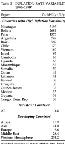
Table 2 shows inflation variability and is organized in the same way as Table 1. Since average inflation and inflation variability are strongly positively correlated, 16 of the top 20 countries in Table 1 are also in the top 20 of Table 2. However, in some cases, such as Chile, the high average inflation rate (107%) reflected one episode of hyperinflation followed by relative stability. In others, such as Colombia, the fairly high average in-

(16)

Table 1 MEAN ANNUAL INFLATION RATE 1970-1990a

Region Rate (%/yr)

High-Inflation Countriesb

Nicaragua 1168

Bolivia 702

Peru 531

Argentina 431

Brazil 288

Vietnam 213

Uganda 107

Chile 107

Cambodia 80

Israel 78

Uruguay 62

Congo, Dem. Rep. 49

Lebanon 44

Lao PDR 42

Mexico 41

Mozambique 41

Somalia 40

Turkey 39

Ghana 39

Sierra Leone 34

All

Industrial Countriesc

Developing Countriesc Africa

Asia Europe Middle East

Western Hemisphere

9.8 16.3 17.4 6.9 19.6 98.6

aBased on GDP deflators. Source: WDI 2001.

b This group includes only countries with 1997 population above 500,000. Ranked by inflation rate.

c Unweighted means.

flation rate (22%) resulted from a long period of moderate, double-digit inflation.

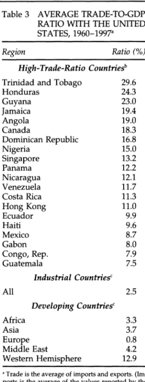
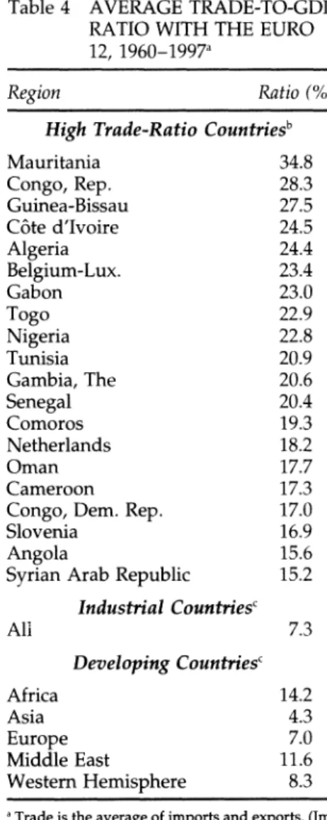
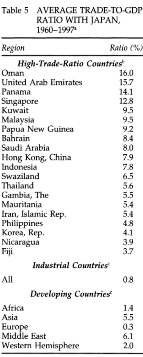
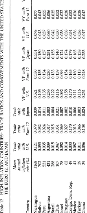
Tables 3, 4, and 5 list for selected countries and groups the average trade-to-GDP ratios16 over 1960-1997 with three potential anchors for cur- rency areas: the United States, the euro area (based on the twelve mem-

16. The trade measure is equivalent to the average of imports and exports. Glick and Rose's (2002) values come from averaging four measures of bilateral trade (as reported for im- ports and exports by the partners on each side of both transactions).

(17)

Table 2 INFLATION-RATE VARIABILITY 1970-1990a

Region Variability (%/yr)

Countries with High Inflation Variabilityb

Nicaragua 3197

Bolivia 2684

Peru 1575

Argentina 749

Brazil 589

Chile 170

Vietnam 160

Israel 95

Cambodia 63

Uganda 63

Mozambique 52

Somalia 50

Oman 46

Lebanon 41

Kuwait 38

Uruguay 38

Guinea-Bissau 37

Mexico 37

Guyana 36

Congo, Dem. Rep 36

All 4.6

Developing Countriesc

Africa 13.9

Asia 14.0

Europe 6.6

Middle East 28.4

Western Hemisphere 251.2

a Standard deviation of annual inflation rates, based on GDP deflators. Source: WDI 2001.

b This group includes only countries with 1997 population above 500,000. Ranked by standard deviation of inflation.

(18)

Table 3 AVERAGE TRADE-TO-GDP RATIO WITH THE UNITED STATES, 1960-1997a

Region Ratio (%)

High-Trade-Ratio Countriesb Trinidad and Tobago 29.6

Honduras 24.3

Guyana 23.0

Jamaica 19.4

Angola 19.0

Canada 18.3

Dominican Republic 16.8

Nigeria 15.0

Singapore 13.2

Panama 12.2

Nicaragua 12.1

Venezuela 11.7

Costa Rica 11.3

Hong Kong 11.0

Ecuador 9.9

Haiti 9.6

Mexico 8.7

Gabon 8.0

Congo, Rep. 7.9

Guatemala 7.5

All 2.5

Africa 3.3

Asia 3.7

Europe 0.8

a Trade is the average of imports and exports. (Im- ports is the average of the values reported by the importer and the exporter. Idem for exports.) Av- erages are for 1960-1997 (when GDP data are not available, the average corresponds to the period of availability). The equations for comovement include only one observation for each pair, cor- responding to the period 1960-1997. The explana- tory variables then refer to averages over time.

Source: Glick and Rose (trade values; WDI 2001 (GDP).

bThis group includes only countries with 1997 population above 500,000. c

Unweighted means.

(19)

318 ? ALESINA, BARRO, & TENREYRO

Table 4 AVERAGE TRADE-TO-GDP RATIO WITH THE EURO 12, 1960-1997a

High Trade-Ratio Countriesb

Mauritania 34.8

Congo, Rep. 28.3

Guinea-Bissau 27.5

Cote d'Ivoire 24.5

Algeria 24.4

Belgium-Lux. 23.4

Gabon 23.0

Togo 22.9

Nigeria 22.8

Tunisia 20.9

Gambia, The 20.6

Senegal 20.4

Comoros 19.3

Netherlands 18.2

Oman 17.7

Cameroon 17.3

Congo, Dem. Rep. 17.0

Slovenia 16.9

Angola 15.6

Syrian Arab Republic 15.2 Industrial Countriesc

All 7.3

Africa 14.2

Asia 4.3

Europe 7.0

aTrade is the average of imports and exports. (Im- ports is the average of the values reported by the importer and the exporter. Idem for exports.) Av- erages are for 1960-1977 (when GDP data are not available, the average corresponds to the period of availability). Source: Glick & Rose (trade values);

WDI 2001 (GDP). For a Euro 12 country, the trade ratios apply to the other 11 countries.

b This group includes only countries with 1997 population above 500,000.

c Underweight means.

(20)

Table 5 AVERAGE TRADE-TO-GDP RATIO WITH JAPAN, 1960-1997a

High-Trade-Ratio Countriesb

Oman 16.0

United Arab Emirates 15.7

Panama 14.1

Singapore 12.8

Kuwait 9.5

Malaysia 9.5

Papua New Guinea 9.2

Bahrain 8.4

Saudi Arabia 8.0

Hong Kong, China 7.9

Indonesia 7.8

Swaziland 6.5

Thailand 5.6

Gambia, The 5.5

Mauritania 5.4

Iran, Islamic Rep. 5.4

Philippines 4.8

Korea, Rep. 4.1

Nicaragua 3.9

Fiji 3.7

All 0.8

Africa 1.4

Asia 5.5

Europe 0.3

a Trade is the average of imports and exports. (Im- ports is the average of the values reported by the importer and the exporter. Idem for exports.) Av- erages are for 1960-1997 (when GDP data are not available, the average corresponds to the period of availability). Source: Glick and Rose (trade values);

WDI 2001 (GDP).

bThis group includes only countries with 1997 population above 500,000.

c Unweigted means.

(21)

bers), and Japan. The GDP value in the denominator of these ratios refers to the country paired with the potential anchor.

The tables show that Japan is an economy that is relatively closed;

moreover, in comparison with the United States and the euro region, Ja- pan's trade is more dispersed across partners. Hence, few countries ex- hibit a high trade-to-GDP ratio with Japan. Notably, industrial countries' average trade share with Japan is below 1%. Among developing coun- tries, oil exporters have a high trade share with Japan, but still below that with the Euro 12. Singapore, Malaysia, Hong Kong, and Indonesia exhibit relatively high trade-to-GDP ratios with Japan (above 7%), but Singapore and Hong Kong trade even more with the United States. For the United States, aside from Hong Kong and Singapore, a good portion of Latin America has a high ratio of trade to GDP. Canada is notable for trading almost exclusively with the United States; its trade ratio is 18%, compared with 1.7% for the Euro 12 and 1.4% for Japan. African countries, broadly speaking, trade significantly more with Europe, but some of them, such as Angola and Nigeria, are also closely linked with the United States.

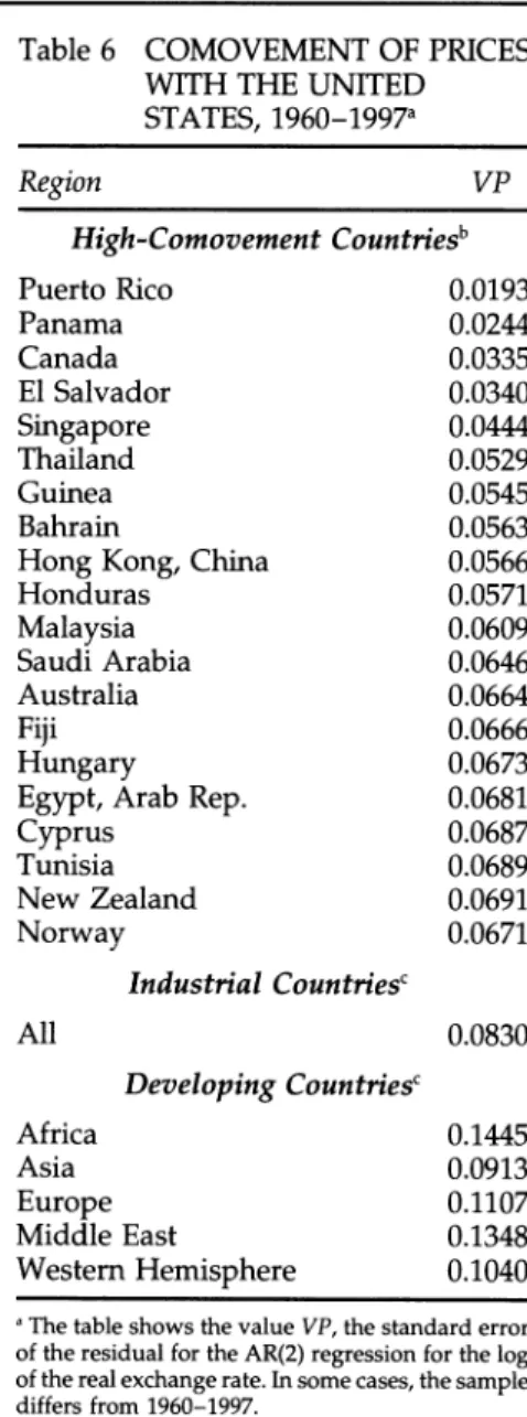
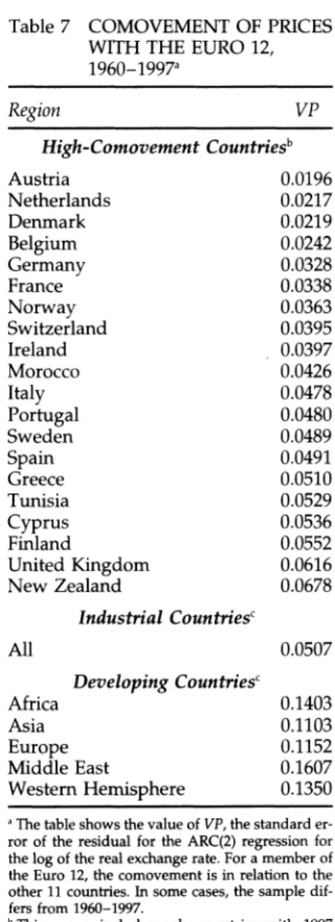
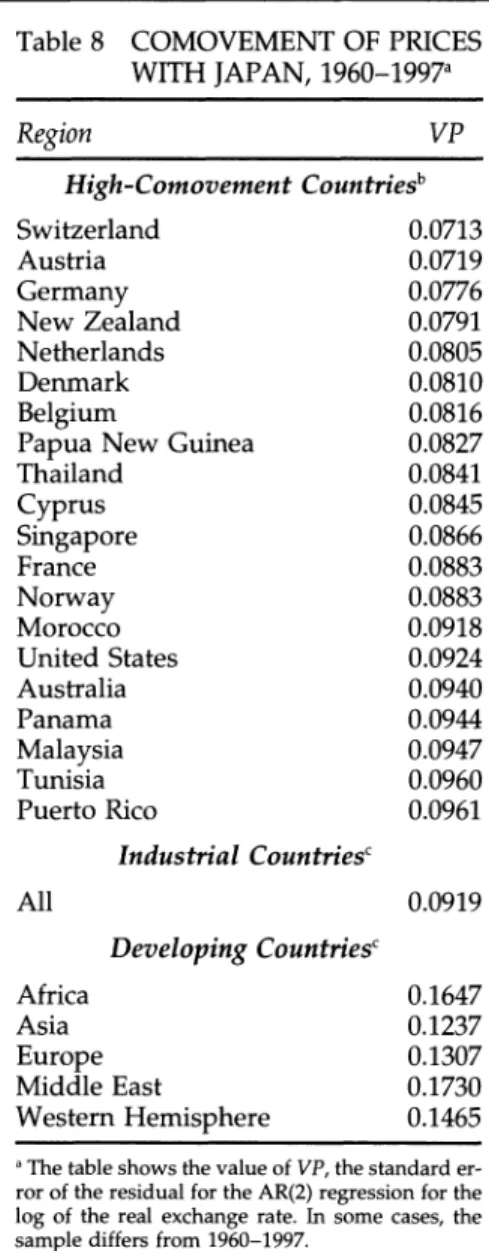
Tables 6, 7, and 8 report our measures of the comovements of prices for selected countries with the United States, the Euro 12 area, and Japan.17 Remember that a larger number means less comovement. Panama and Puerto Rico, which use the U.S. dollar, have the highest comovements of prices with the United States. These two are followed by Canada and El Salvador, which has recently dollarized. Members of the OECD have fairly high price comovements with all three of the potential anchors (which are themselves members of the OECD). For Japan, the countries that are most closely related in terms of price comovements lack a clear geographical distribution. For the Euro 12, the euro members and other western European countries have a high degree of price comovement.

African countries also have relatively high price comovements with the Euro 12, higher than that with the United States.

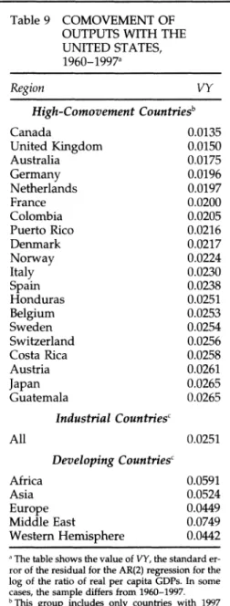
Tables 9, 10, and 11 report our measures of the comovements of outputs (per capita GDPs) for selected countries with the United States, the Euro 12 area, and Japan.18 The general picture is reasonably similar to that for prices. Note that all of the OECD countries have relatively high output comovements with the three anchors, particularly with the Euro 12. Ja- pan's business cycle seems to be somewhat less associated with the rest of the world: even developing countries in Asia tend to exhibit, on aver- age, higher output comovements with the Euro 12. The regional patterns

17. Recall that we compute comovements only for pairs of countries for which we have at least 20 annual observations.

18. As for prices, we consider only pairs of countries for which we have at least 20 observations.

(22)

Table 6 COMOVEMENT OF PRICES WITH THE UNITED

STATES, 1960-1997a

Region ^VP

High-Comovement Countriesb

Puerto Rico 0.0193

Panama 0.0244

Canada 0.0335

El Salvador 0.0340

Singapore 0.0444

Thailand 0.0529

Guinea 0.0545

Bahrain 0.0563

Hong Kong, China 0.0566

Honduras 0.0571

Malaysia 0.0609

Saudi Arabia 0.0646

Australia 0.0664

Fiji 0.0666

Hungary 0.0673

Egypt, Arab Rep. 0.0681

Cyprus 0.0687

Tunisia 0.0689

New Zealand 0.0691

Norway 0.0671

All 0.0830

Africa 0.1445

Asia 0.0913

Europe 0.1107

Middle East 0.1348

a The table shows the value VP, the standard error of the residual for the AR(2) regression for the log of the real exchange rate. In some cases, the sample differs from 1960-1997.

(23)

Table 7 COMOVEMENT OF PRICES WITH THE EURO 12, 1960-1997a

Region VP

Austria 0.0196

Denmark 0.0219

Belgium 0.0242

Germany 0.0328

France 0.0338

Norway 0.0363

Switzerland 0.0395

Ireland 0.0397

Morocco 0.0426

Italy 0.0478

Portugal 0.0480

Sweden 0.0489

Spain 0.0491

Greece 0.0510

Tunisia 0.0529

Cyprus 0.0536

Finland 0.0552

United Kingdom 0.0616

New Zealand 0.0678

All 0.0507

Africa 0.1403

Asia 0.1103

Europe 0.1152

Middle East 0.1607

aThe table shows the value of VP, the standard er- ror of the residual for the ARC(2) regression for the log of the real exchange rate. For a member of the Euro 12, the comovement is in relation to the other 11 countries. In some cases, the sample dif- fers from 1960-1997.

b This group includes only countries with 1997 population above 500,000.

(24)

Table 8 COMOVEMENT OF PRICES WITH JAPAN, 1960-1997a

Region VP

Austria 0.0719

Germany 0.0776

New Zealand 0.0791

Denmark 0.0810

Belgium 0.0816

Papua New Guinea 0.0827

Thailand 0.0841

Cyprus 0.0845

Singapore 0.0866

France 0.0883

Norway 0.0883

Morocco 0.0918

United States 0.0924

Australia 0.0940

Panama 0.0944

Malaysia 0.0947

Tunisia 0.0960

Puerto Rico 0.0961

All 0.0919

Africa 0.1647

Asia 0.1237

Europe 0.1307

Middle East 0.1730

a The table shows the value of VP, the standard er- ror of the residual for the AR(2) regression for the log of the real exchange rate. In some cases, the sample differs from 1960-1997.

(25)

Table 9 COMOVEMENT OF OUTPUTS WITH THE UNITED STATES, 1960-1997a

Region VY

Canada 0.0135

United Kingdom 0.0150

Australia 0.0175

Germany 0.0196

France 0.0200

Colombia 0.0205

Puerto Rico 0.0216

Denmark 0.0217

Norway 0.0224

Italy 0.0230

Spain 0.0238

Honduras 0.0251

Belgium 0.0253

Sweden 0.0254

Costa Rica 0.0258

Austria 0.0261

Japan 0.0265

Guatemala 0.0265

All 0.0251

Africa 0.0591

Asia 0.0524

Europe 0.0449

Middle East 0.0749

Western Hemisphere 0.0442 The table shows the value of VY, the standard er- ror of the residual for the AR(2) regression for the log of the ratio of real per capita GDPs. In some cases, the sample differs from 1960-1997.

b This group includes only countries with 1997 population above 500,000.