Chemistry of salts in aqueous solutions:Applications, experiments, and theory*

(1)

doi:10.1351/PAC-CON-11-01-07

Chemistry of salts in aqueous solutions:

Applications, experiments, and theory*

Wolfgang Voigt

^‡

TU Bergakademie Freiberg, Institut für Anorganische Chemie, Leipziger Strasse 29, D-09596 Freiberg, Germany

Abstract:Salts comprise a very large and important group of chemical compounds. Natural occurrence of salts and industrial processes of their recovery, conversion, purification, and use depend on solubility phenomena and their chemistry in aqueous solutions, mostly in multi-ion systems. Modeling of these processes as well as developing new ones requires knowledge of the properties of the aqueous salt solutions in extended T-p-x ranges including a growing number of components in solutions (CO₂, SO₂, lithium salts, salts of rare earth metals, actinides, etc.). At least for the thermodynamic properties, the general accepted methodology is to use thermodynamic databases of aqueous species and solids in combination with an appropriate ion-interaction model to perform equilibrium calculations for species distributions in solution and phase equilibria. The situation in respect to available thermodynamic models and data for their parameterization is discussed at selected examples.

Thereby, the importance of accurate experimental determinations of phase equilibrium data for derivation of model parameters is emphasized. Furthermore, it is concluded that experimental investigations should follow a chemical systematic. Simple physical models or quantum chemical calculations cannot predict unknown quantities in the databases with sufficient accuracy.

Finally, solubility changes in salt–water systems at enhanced temperatures are considered. Systems, which can be considered as molten hydrates, display interesting phase behavior and chemical reactivity as protic ionic liquids. The latter can be exploited in chemical syn- theses to substitute mixtures of concentrated acids like HNO₃/H₂SO₄ by simple salts like ferric nitrate.

For an understanding of the chemical and phase behavior of water–salt systems in terms of structure–property relations, a renaissance of chemical guided basic investigations of such systems would be worthwhile.

Keywords: Brunauer–Emmett–Teller (BET) model; molten salt hydrates; oceanic salts; poly- halite; thermodynamic models.

INTRODUCTION

The chemistry of salts in aqueous solutions concerns first of all processes of its dissolution and crystallization, hydrolysis, and formation of complex ions in solution. The combination of metal cations with typical inorganic anions as halide, sulfate, nitrate, phosphate, etc. yields a very large number of

*Paper based on a presentation made at the 14^thInternational Symposium on Solubility Phenomena and Related Equilibrium Processes (ISSP-14), Leoben, Austria, 25–30 July 2010. Other presentations are published in this issue, pp. 1015–1128.

‡E-mail: Wolfgang.Voigt@chemie.tu-freiberg.de

(2)

compounds with salt-like properties, that is properties dominated by ions. The class of salts covers a wide spectrum: from NaCl, gypsum (CaSO₄ⴢ2H₂O), anhydrite (CaSO₄), saltpeter (NaNO₃), and cryo- lite (Na₃AlF₆) to salts of heavy metals or of noble metals. In geology, environmental sciences, medi- cine, and industrial processes many problems are related to the question of the solubility of salts. This question asks for the ion combination, which will form a solid salt from an aqueous solution of certain composition and temperature. Every textbook on general and inorganic chemistry describes salts as ionic compounds crystallizing in ionic lattices with a certain lattice energy. Dissolving these salts in water requires that the lattice energy is overcome by the process of ionic hydration. Both quantities are then used to explain the tendencies in the solubility for simple salts like alkaline metal halides or alkaline earth metal sulfates often in relation to the Haber–Born cycle [1]. This picture is only suited to get a rough idea about factors like ion charge/radius ratio having influence on the solubility of salts. Besides the intrinsic properties of the solids (lattice enthalpy, entropy) the solubility of salts in water or in solutions containing other ions depends on the ion–water and ion–ion interactions. These interactions are changing very sensitively with concentration, composition, and temperature. At present, chemistry can still not give a quantitative answer by means of definite structural models [2]. Solubility relations of different salts in mixed ionic solutions form also the basis for an understanding of their existence and sta- bility in contact with aqueous solutions.

The first systematic investigation of this kind was realized by J. H. van’t Hoff, the first winner of a Nobel prize in chemistry in 1901 (Fig. 1), whose centenary of death we remember in 2011. By con- sequently applying state-of-the-art theory of chemical thermodynamics and equilibrium, he and his co- workers developed within 12 years research a nearly complete scheme of the composition and temperature conditions for the formation of the various salt phases (hydrated and anhydrous simple salts, double salts, triple salts) from aqueous solutions of the oceanic system, which comprises the ions Na⁺, K⁺, Mg²⁺, Ca²⁺, Cl^–, and SO₄^2–. The results of the 52 papers were summarized in the famous book Investigations on the Conditions of Formation of the Oceanic Salt Deposits, especially of the Stassfurt Deposit(see Fig. 2). At the same time, this was the first systematic investigation of a multi component salt–water system, which was highly needed at that time for a more effective exploration of potash deposits and its recovery to produce potash fertilizers. The work of van’t Hoff was continued by D’Ans [3], Autenrieth [4,5], and Emons [6,7] and is continued to the present [8–10]. More than 100 years Fig. 1 Jacobus Henricus van’t Hoff and the document of the Swedish Academy of Science awarding him the Nobel Prize in Chemistry.

(3)

research on this salt system has steadily improved the technology in recovery of mineral fertilizers, the understanding of formation of salt deposits, and the production of basic chemicals as part of the extended oceanic system including carbonates, H⁺and OH^–.

SALT–WATER SYSTEMS IN MODERN APPLICATIONS

New aspects of applications with the need for detailed knowledge of solubility, solution equilibria, and properties in the oceanic salt system are the storage of nuclear wastes in geological salt formations as in northern Germany (Gorleben, Morsleben) or in New Mexico, USA (Carlsbad WIPP site), storage of inorganic toxic waste in old salt mines (Teutschenthal, Germany), CO₂sequestration in highly saline aquifers of large depths, and exploitation of geothermal brines. These new tasks require knowledge of the phase behavior and solution properties at extended temperature and pressure ranges, the inclusion of more and more components as CO₂, heavy metals, actinides, acids and bases, and Li⁺. The latter ion recently became a very important issue for the recovery of lithium salts from brines of salt flats and lakes in South America (Chile, Argentina, Bolivia) and Asia (West China) to ensure a sufficient production of Li₂CO₃for large lithium batteries in automotive and other applications. The brines located in the salt crusts contain between 300–4000 ppm Li⁺. The concentration is enhanced by solar evapora- tion. At the same time, huge amounts of other salts have to be crystallized [11] and separated exploit- ing the multicomponent solubility equilibria (Fig. 3).

Another topic concerns weathering of historical and modern buildings. It is often controlled by crystallization and dissolution of salts at changing humidity of the surrounding air. To understand these processes, detailed data on phase diagrams and properties (water activity, partial molar volumes) of mixed solutions of alkaline and alkaline earth metal chlorides, nitrates, and sulfates are needed [12,13].

Fig. 2 Cover of the book Untersuchungen über die Bildungsverhältnisse der Ozeanischen Salzablagerungen insbesondere des Stassfurter Salzlagers, summarizing the papers of van’t Hoff edited by Precht and Cohen, 1912.

(4)

Another topic where the chemistry of salt–water systems is asked for concerns interplanetary science. New observations of Mars missions gave evidence for aqueous salt solutions existing at very low temperatures (180–250 K). The questions arise, which cryotectic water–salt mixtures can be formed down to about 200 K, what properties can we expect from these solutions, and could it be a possible environment for life? To answer these questions, a large number of salt–water systems have to be considered [14].

Modern applications concern of course all the hydrometallurgical processes for recovery and purification of zinc, aluminum, and heavy metals like copper, nickel, cobalt, etc. The control of leach- ing and solid–liquid separation processes require a more accurate description of phase and chemical equilibria and the kinetics to reach these equilibria [15].

Environmental sciences need more accurate equilibrium data in order to make use of the sensi- tivity and accuracy of modern methods of concentration monitoring.

Summarizing, it can be stated that modern needs in the chemistry of salt–water systems consist on one hand in a fine-tuning of the models for property descriptions and on the other hand in predictions when extending temperature, pressure, or system components.

SOLUTION MODELS AND THERMODYNAMIC DATABASES

Starting with van’t Hoff, further development in the theory of salt solutions or more general electrolyte solutions focused on the physical description of the long-range ion–ion interactions [16]. Combined with ion-specific, short-range interaction terms, equations were formulated describing the concentration dependence of activity coefficients of salt components [17], osmotic coefficients, or more general the excess Gibbs energy of mixing [18–21]. Still the most popular approach for the thermodynamic treat- ment of concentrated electrolyte solutions represents Pitzer’s ion interaction model [22]. It is based on some fundamental considerations on virial equations for electrolyte solutions, a restriction to the sec- ond and third virial coefficient with a suited choice of the mathematical form of ionic strength dependence. Thus, the model is able to describe the thermodynamic properties of electrolyte solutions up to Fig. 3Salar de Uyuni (Bolivia, 10.000 km²) with an average lithium content of 500–600 ppm Li⁺/L in the inter- granular brine below the salt surface. Inset: brine cavity 40 cm below surface and main ions in solution with amounts of salts to be crystallized for the production of 1 t of Li₂CO₃.

(5)

ionic strengths of approximately 6–10 mol/kg H₂O, when model parameters are estimated from appropriate binary and ternary salt–water systems. For a given temperature and a typical system like NaCl–KCl–H₂O, 3 parameters for every binary system (NaCl–H₂O, KCl–H₂O) and 2 additional empirical parameters are required for the ternary system, that is 8 parameters in this case. All interactions in the higher-component systems are calculated using only parameters from the corresponding binary and ternary systems. Nevertheless, for the hexary oceanic salt system the parameters have to be estimated from experimental data of 8 binary and 16 ternary systems, which gives 56 isothermal parameters and 2 additional parameters for the 2-2 valent electrolytes MgSO₄and CaSO₄. Using these parameters, the activity coefficients of saturated salt solutions can be calculated and thus the thermodynamic solubility constants. For the most important 35 salt phases it has been done for the oceanic salts [23]. Pitzer parameters and solubility constants form a data set stored in a thermodynamic database, which in con- nection with appropriate equilibrium calculation codes (ChemSage, ChemApp, FACTSAGE, EQ3/6, PHREEQC, GEMS, MINEQL+) allow simulation of phase equilibria of complex composed salt–water systems. In a similar way, also parameters for speciation equilibria in homogenous solutions (complex formation) with interactions of the corresponding complex ions and their equilibrium constants are extracted from experimental data [24].

Pitzer’s theory gives no hint for the temperature dependence of the model parameters and thus entirely empirical equations are used. For a temperature interval from 0 to about 200 °C, up to 8 temperature coefficients are necessary for every Pitzer parameter. The same is valid for the solubility constants. Databases containing such temperature-dependent parameters enable calculation also for enthalpic effects. However, the predictive power of the Pitzer model is limited, especially when the ionic strengths are higher than 6 molal.

The computing power of personal computers or laptops is sufficient to perform equilibrium calculations with hundreds of species and phases in seconds. Thus, the current state of the art to study geochemical and industrial processes consists in thermodynamic modeling and simulation using a suited database and program code. Efforts are being made to couple equilibrium calculations with transport codes [25]. In this case, computing time for the equilibrium states becomes critical.

The large number of parameters is not a limiting factor in computer calculations. The limitation has to be seen in the availability of experimental data for their estimation. Thus, for solutions formed from combinations of the most important of 28 cations and 16 anions, activity data for 448 binary and 9408 ternary systems have to be provided and approximately 22.000 parameters have to be extracted from the available experimental data for one temperature. Only for a limited number of ternary systems are such data available for one temperature, even worse is the situation when temperature ranges have to be considered. Database projects, where existent data from literature are gathered to extract model parameters, have been reviewed recently [26].

Therefore, constant efforts are directed to develop models with a smaller number of adjustable parameters. However, applicability is mostly tested only for binary salt–water systems [27–31]. One general approach combines typical nonelectrolyte models such as NRTL, UNIQUAC, or UNIFAC models with an extended Debye–Hückel term [32–39].

Extensive demonstrations for application of an extended NRTL model for salt–water systems are given by Iliuta and Thomsen [35]. As long as temperature-dependent models are considered the advan- tage of an apparently smaller number of parameters in the solution model is often counteracted by abnormal many temperature coefficients of the solubility constant. Often the existence range of a salt hydrate or double salt is less than 15 K, however, the solubility constant is modeled with 5 temperature coefficients [35]. Other types of model use physical reference models like MSA (mean spherical approximation), integral equation approach, or others: reviewed in [40].

Another way to derive missing interaction coefficients, for instance, in a Pitzer model is to generate “quasi-experimental” data by the use of mixing rules like those of Zdanovskii or Young [41–43]

Thermodynamic standard-state properties of ions in water at 298 K can be found in [44–47]. For extended temperatures and pressures the correlation from Helgeson, Kirkham, and Flowers (HKF

(6)

model) [48,49] is often used, where the values generated by the HKF model can easily be accessed by means of the software package SUPCR92 [50]. Also, more simple correlations as proposed by Cobble and co-workers [51,52] or the coulombic compensation principle [24,53] can be used to estimate standard data for high temperatures.

In online databases these data are often easily accessible [26]. However, the user has to ensure (sometimes supported by the database itself as in THEREDA) that standard data, speciation, and activity models are consistent with each other. Despite consistency issues and uncertainties in validity ranges of model parameters, etc. the community of users routinely applying packages consisting of solution model, databases, and calculation codes to handle aqueous chemistry problems is ever growing.

Therefore, there is a strong focus to expand the databases and to improve the codes and their user inter- faces.

DATA SOURCES AND EXPERIMENTS

The most important types of experiments from which parameters for thermodynamic models are estimated are

a) isopiestic measurements [54]

b) vapor pressure measurements [55–57]

c) galvanic cells in dilute aqueous solutions [58–61]

d) measurements of heat capacities [62–68] and heat of dilution [69–71] or dissolution [72]

e) pH [73], spectrophotometric mesurements [74–77], Raman and NMR spectroscopy for speciation equilibria [78,79]

f) determination of solid–liquid equilibria (solubilities) [80]

Experiments of types a–e are normally performed in undersaturated solutions providing properties of the solution only. Combined with determinations of solid–liquid equilibria thermodynamic quantities of the solid phases can be derived. In principle (and most basic) the latter information can be obtained from enthalpy of dissolution of the solid-phase and low-temperature heat capacity measurements. However, the overwhelming majority of Gibbs energy of formation data of salts and its hydrates tabulated in standard data books [46,47] have been derived from solubility data. Without accurate solubility data also most of the formation data would be inaccurate.

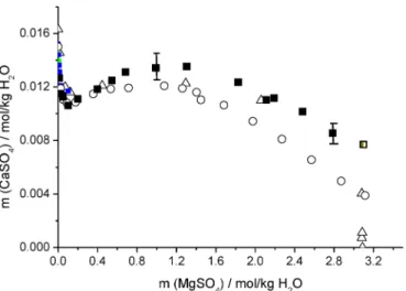
Particularly in the case of solubility determinations often very old papers have to be studied, because the study of solubility in aqueous salt systems in contemporary chemistry is not considered as scientifically interesting. One actual example represents the solubility equilibria of polyhalite, a wide spread in rock salt formations triple salt mineral, K₂SO₄ⴢMgSO₄ⴢ2CaSO₄ⴢ2H₂O. At the standard temperature of 298 K, data only from van’t Hoff [81] or [82] are available. In order to accomplish a thermo - dynamic model to describe the compositions of solutions, where polyhalite can be in equilibrium besides the solubility product of polyhalite itself also the Pitzer parameters for the Mg²⁺–Ca²⁺and Mg²⁺–SO₄^2––Ca²⁺interaction have to be known at high concentrations of MgSO₄. The latter can be best determined from solubilities of gypsum in MgSO₄ solutions. Harvie, Möller, and Weare estab- lished the well-known in the geochemical community Pitzer equation based seawater model for T = 298 K [83]. In their data compilation they had to rely on solubility determinations of gypsum by Cameron [84] from the year 1906 for the description of the Mg²⁺–SO₄^2––Ca²⁺interaction. At that time no suited analytical method was available for the determination of Ca²⁺concentrations in high concentrated magnesium salt solutions. The difference between the old and new data is illustrated in Fig. 4.

The consequences of new data are illustrated for the existence range of polyhalite in solutions of potas- sium and magnesium sulfate at 298 K as shown in Fig. 5. Implemented in a new Pitzer model of the hexary oceanic salt system (available from <www.thereda.de>), a much larger composition range is calculated for the existence of polyhalite at 298 K. This has consequences for the geochemical interpreta- tion of brine analyses. Also, we conclude that the lower formation temperature of polyhalite in contact

(7)

with solution can be lower than 286 K as was predicted by van’t Hoff [81] and never adjusted until present days. First findings of polyhalite from drillings in the Salar de Uyuni, where temperatures are well below 286 K, seem to confirm this conclusion.

FORMATION OF DOUBLE SALTS AND SALT HYDRATES

The prediction of the crystallization fields of the various hydrate types of a salt or double salt represents a long-standing issue. In past times the preferred approach was the direct phase equilibrium experiment.

For a certain class of salts or their combinations, the phases in equilibrium were separated and chemi- Fig. 4Solubility of gypsum according to Cameron 1906 [84] (○), Kolosov [85] () and Wollmann 2010 [86] (^),

error bars.

Fig. 5Crystallization field of polyhalite (Ph) in the system K₂SO₄–MgSO₄–CaSO₄–H₂O at 298 K; thin lines = calc. with Pitzer model based on new solubility data [86], thick-lined polygon = polyhalite field calc. with model of HMW [83], stars = existence triangle for polyhalite according to experiments of Van Klooster [82].

(8)

cally analyzed. Guided by some correlations of chemical parameters like ionic radius, chemical hard- ness, and softness [87] or ligand field stabilization energies, the comparison of a series of systems and their phase diagrams led to conclusions about the possible existence of double salts in analogous systems not investigated at time. Of course, such correlations were more or less qualitative. The situation has changed dramatically in the last 20 years. Progress in methods for X-ray crystal structure analysis made it possible to discover a large number of new crystal phases in nature and in the lab. Often also the composition of known salts are determined more accurately as, for example, for the

“MgSO₄ⴢ12H₂O”, which is now meridianite, MgSO₄ⴢ11H₂O, [88,89], similar for kainite [90] or loeweite [89]. Thus, the situation arose that hundreds of double salt phases are known structurally but no thermodynamic data of formation are available and the conditions of their formation or crystallization are unknown. In order to fill such data gaps in thermodynamic databases, several estimation methods have been proposed as, for instance, by Jenkins and Glasser [92–94] for ionic hydrates. In essence, the authors make use of linear relations of the type

{Δ_fH°_hydrate, Δ_fG°_hydrate} = {Δ_fH°_anhydrate, Δ_fG°_anhydrate} + aⴢn_H

2O (1)

where Δ_fH°, Δ_fG° denote the respective standard enthalpies and Gibbs energies of formation, n_H

2Othe number of moles water in the hydrate, and the slope “a” represents the increment per mol water. The data fulfill the equation within a scatter of 25 kJ/mol. Thus, this method yields quite rough estimates.

Difference rules of this type do not consider structural features of the solids, and due to the linearity of the formation quantities, hydrates with any number of n_H

2Owould be predicted as stable for a given salt.

Another recently published (but not really new) approach concerns the estimation of solubility constants of double salts, K_L(DS), from their single component salts [95,96] by means of eq. 2.

K_L(DS) = K_L(1)ⴢK_L(2) (2)

Since the relation 3 is valid eq. 2 implies the additivity rule of the Gibbs energies of

–RTⴢln[K_L(i)] = Δ_LG°(i) (3)

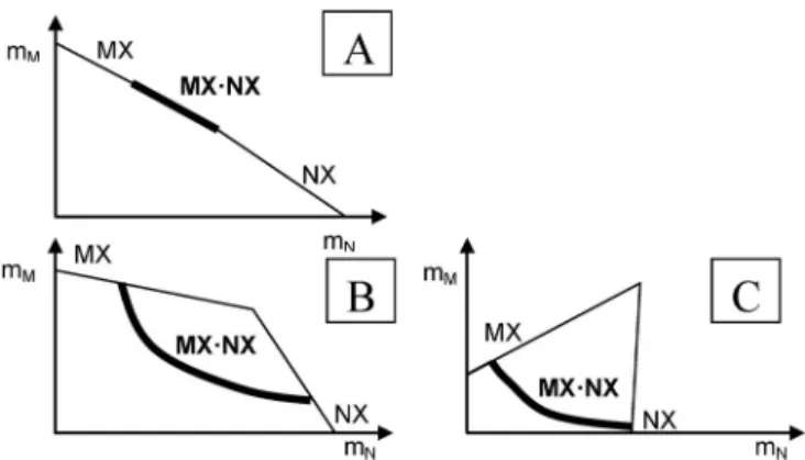
formation of the component salts. This means, however, an absence of a driving force to form the double salt. The apparent confirmation of this “rule” by comparing calculated and experimentally found solution concentrations is a consequence of the form of some solubility diagrams as shown in Fig. 6 as well as of the accuracy of chemical analysis. In the case of type A, the solution composition in equilibrium with the double salt is not much different from a solution composition of the mixture of the single salts, and hence the “rule” is apparently valid. Not so in cases of types B and C, where the forma-

Fig. 6Types of solubility isotherms of systems MX–NX–H₂O with double salt formation MXⴢNX, thick line = crystallization branch of double salt, thin lines = crystallization branches of single salts MX, NX.

(9)

tion of the double salt decreases the total salt concentration considerably in relation to the extrapolated single salt branches in the diagram.

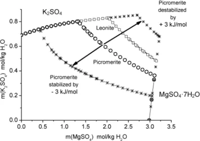
Double salts of the type M₂SO₄ⴢM'SO₄ⴢ6H₂O, Tutton’s salts, belong to the most extensively investigated double salt hydrates. To predict which combination of M and M' form stable salts in contact with aqueous solutions, one could try to estimate the Gibbs energy of formation from aqueous ions and use one of the above-mentioned programs and solution models to calculate the crystallization branches of possible double salts. In Figs. 7a,b, the known Gibbs energies of formation for M = K are correlated with the position in the periodic table (7a) and the radius of ion M'²⁺(7b). As can be seen from the graphs for Mn²⁺, V²⁺, and Cr²⁺the correlation would yield negative values of Gibbs energies of formation, however, with an uncertainty of approx. ±3 kJ/mol. The influence of such a variance of Δ_fG°(DS) is demonstrated in Fig. 8 for M'²⁺= Mg²⁺. The changes in the solubility isotherms are dras- tic, and other phases such as leonite overlap in the field of uncertainty. There are also efforts to apply quantum chemical methods to predict the existence of solid phases [97,98]. However, for double salt predictions they are too inaccurate.

Fig. 7Correlation of the standard Gibbs energies of formation of picromerite, K₂SO₄ⴢMSO₄ⴢ6H₂O, from aqueous ions at 298 K and prediction for M = Mn. Ionic radius with coordination number of 6.

Fig. 8Effect of an uncertainty of ±3 kJ/mol in the Gibbs energy of formation of picromerite on the solubility curve at 298 K. Open circles = solubility of picromerite, stars = calculated solubility of picromerite with reduced or enhanced Gibbs energy of formation, open rectangles = solubility of leonite; picromerite = K₂SO₄ⴢMgSO₄ⴢ6H₂O, leonite = K₂SO₄ⴢMgSO₄ⴢ6H₂O.

(10)

Thus, much more accurate data of Δ_fG°(DS) are needed for solubility predictions of unknown double salts. Presently available estimation methods are not sufficient for this purpose. Table 1 lists all known double salts of the type M₂SO₄ⴢM'SO₄ⴢ6H₂O. The K–Mn combination could not be prepared until now [99]. Our own investigation of the system K₂SO₄–MnSO₄–H₂O at 298 and 313 K revealed the formation of the double salts K₂SO₄ⴢ3MnSO₄ⴢ5H₂O, K₂SO₄ⴢMnSO₄ⴢ2H₂O, K₂SO₄ⴢMnSO₄ⴢ1.5H₂O, K₂SO₄ⴢMnSO₄ⴢ4H₂O, and K₂SO₄ⴢ2MnSO₄ [100], but no Tutton’s type.

Maybe the latter can be found at lower temperatures, however, already at ambient temperatures equi- libration times of 1–2 months had to be applied to obtain the equilibrium solid phases.

Table 1Evidence for the existence of Tutton’s salts M₂SO₄ⴢM'SO₄ⴢ6H₂O after Nalbandyan [99]; number of PDF entries, “no success” means no successful attempts for preparation, “no info” means no information at all.

M'⁺

M²⁺ K Rb Tl NH₄ Cs

Ni 3 2 1 7 2

Ru 1 no info no info no info no info

Mg 2 2 1 5 2

Cu 2 2 2 6 2

Co 4 2 1 4 2

Zn 3 2 1 5 2

Fe 1 2 1 2 2

V no info no info no info 2 no info

Cr no info no info no info 1 no info

Mn no success 1 1 2 2

Cd no info no info no success 2 no success

PROPERTIES OF SALT SOLUTIONS AT ENHANCED TEMPERATURES

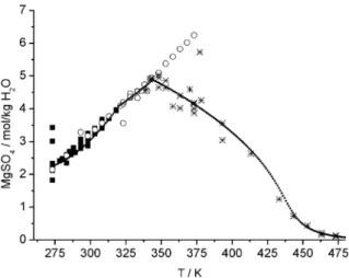
Enhancing the temperature the solubility of salts can increase or decrease, for MgSO₄ both can be observed as shown in Fig. 9. At temperatures near 200 °C MgSO₄becomes a sparingly soluble salt comparable with CaSO₄. The negative temperature coefficient of solubility is caused by strongly

Fig. 9 Temperature dependence of the solubility of MgSO₄, symbols: experimental data (filled rectangles:

heptahydrate, rhombus: hexahydrate, stars: monohydrate, line: calculated with THEREDA model).

(11)

decreased ion hydration and ion association. Addition of another electrolyte turns the negative temperature coefficient into a positive one if sufficiently high concentrations are reached.

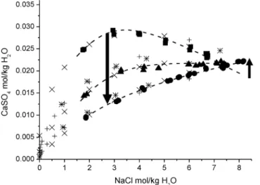
This topic was thoroughly discussed by Valyashko [101]. This phenomenon was recently also confirmed the solubility of CaSO₄, anhydrite, in solutions of NaCl at enhanced temperatures [102], which is nicely visible at the crossing point of the solubility isotherms at 7.0 mol/kg H₂O (see Fig. 10).

In mixed salt solutions at very high concentrations due to the coordination competition of cations for water and anions, peculiar behavior can occur as is illustrated for the system KCl–MgCl₂–H₂O in Fig. 11. The course of the solubility isotherms of KCl in dependence on the concentration of MgCl₂ passes a minimum and at extremely high MgCl₂concentration, in the range of molten hydrates [103]

Fig. 10Solubility isotherms of anhydrite at 373 (^{), 423 (}), and 473 () K in dependence on NaCl concentration;

large symbols: data [102], arrows: direction of temperature coefficient of solubility.

Fig. 11Solubility isotherms in the system KCl–MgCl₂–H₂O at 160 °C (*), 170 °C (○), and 180 °C (^{) [105].}

Arrow and hatched area: supersaturation of KCl when water is added to a saturated solution at point A. other solids:

C = carnallite, KClⴢMgCl₂ⴢ6H₂O, M1 = MgCl₂ⴢ4H₂O, M2 = solid solution MgCl₂ⴢ2H₂O–KClⴢMgCl₂ⴢ2H₂O, M3 = KClⴢMgCl₂ⴢ2H₂O, M4 = 1.5 KClⴢMgCl₂ⴢ2H₂O.

(12)

solubility increases again due to action of KCl as a chloride ion donator for MgCl₂, which forms chloro- complexes [104]. This has the effect that at T ≥ 160 °C and m(MgCl₂) > 130 mol/1000 mol H₂O (>7.2 mol/kg H₂O) a very soluble salt such as KCl can be crystallized by addition of water (Fig. 11), which is quite surprising.

The thermodynamic properties in the range of molten salt hydrates are successfully described by means of the modified Brunauer–Emmett–Teller (BET) model [106–111]. This model uses only two parameters for every salt component (maximum hydration number and the adsorption energy of water at the salt component). Often the temperature dependence of these parameters is sufficiently described by a linear or quadratic function. When salt–salt interactions are strong (complex formation) the simple BET model cannot be used.

Recently, it was shown that models with a small number of parameters can be formulated, when the enthalpy and entropy of step-wise formation of hydrated ions and anionic complexes are interrelated in reaction chains [112]. Formation data of the anhydrous species can be estimated from thermo - dynamic measurements in anhydrous molten mixtures at much higher temperatures. An example of the description quality is given for the system KCl–MgCl₂–H₂O in Fig. 12. For this system, enthalpic and entropic parameters for the following species were derived from all available thermodynamic data in the aqueous and molten anhydrous system (for details, see [110]): MgCl₂(H₂O)_n (i = 0,...,6), Mg(H₂O)²⁺_6+n, K₂(MgCl₂)_nCl₂ (n= 1,..,5), K(H₂O)⁺, K(H₂O)₂⁺, KMgCl₃(H₂O)₃, KMgCl₃(H₂O)₄. Considering the large interval of composition and temperature a fairly good description of the thermodynamic quantities of liquid phase could be achieved with 20 parameters. For the phase diagrams only the formation enthalpy and entropy of the solid hydrates had to be adjusted.

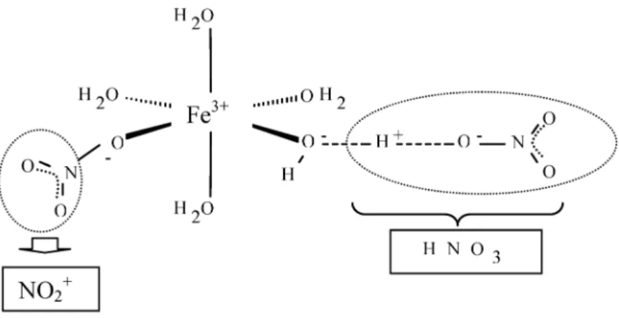
Further peculiarities of molten salt hydrates concern the acidity and reactivity. The acidity of simple solutions like ZnCl₂or Al(NO₃)₃become comparable with strong mineral acids like HCl, when the molar water/salt ratio is diminished below 6 [113]. In these liquids, noble metals as gold can be dis- solved at temperatures below 100 °C [114]. In essence, molten salt hydrates represent protic ionic liquids, the reactivity of which can be controlled by the water content and specific choice of cation-anion combination. An idea of the structural situation and resulting reactivity can be gained from Fig, 13 for molten ferric nitrate pentahydrate. The water molecules are strongly polarized between nearest-neigh- Fig. 12Simultaneous description of the phase diagram of the system KCl–MgCl₂–H₂O (A) between 373–523 K and the thermodynamic properties of the anhydrous molten system KCl–MgCl₂at 1073 K (B) applying a reaction chain model [112].

(13)

bor cations and anions, such that proton transfer is facilitated and an activity of HNO₃results. Direct coordination of NO₃^– at Fe³⁺can generate a situation, which is comparable with the formation of a nitryl cation. These effects are obviously responsible for the nitrating ability of this molten hydrate. In this medium, toluene can be nitrated to mono- and dinitro-toluene [115], a reaction for which, in general, mixtures of concentrated sulfuric and nitric acid are needed.

CONCLUSIONS

Modern science and technology requires accurate property data of aqueous salt solutions at extending ranges of temperature, pressure, and composition. At the same time, a growing number of ionic con- stituents have to be considered. The computing power of personal computers is sufficient to calculate complex solubility and speciation equilibria of multicomponent water–salt systems by means of contemporary equilibrium calculation codes. However, the results are limited by the underlying thermo - dynamic databases and parameters of solution models. The limitations concern

• the accuracy of the description of experimental data,

• the available model coefficients for the various ion–ion interactions,

• the standard data for solid salts, particularly hydrates and double salts, and

• the ranges of temperature and pressure.

Current physical models cannot predict missing data for solid phases, particularly hydrates and double salts, with the required accuracy. For extrapolations of mixed solution properties toward higher concentrations, simple mixing rules such as Zdanovskii’s or Young’s rules should be preferred to extrapo- lation of validity ranges of more complex models.

Application-oriented experimental programs are set up to fill some of the data gaps. However, in parallel a renaissance of systematic physico-chemical investigations of electrolyte systems would accel- erate the development of structure–property-related models suited for predictions.

ACKNOWLEDGMENTS

Continuous financial support from the German Federal Ministry of Education and Research and the German Federal Ministry of Economy is acknowledged.

Fig. 13Possible structural situation in molten ferric nitrate pentahydrate to explain the nitrating effect.

(14)

REFERENCES

1. M. Ladd. Chemical Bonding in Solids and Fluids, Ellis Horwood, New York (1994).

2. W. Kunz (Ed.). Specific Ion Effects, World Scientific, Singapore (2010).

3. J. D’Ans. Die Löslichkeitsgleichgewichte der Systeme der Salze ozeanischer Salzablagerungen, Verlagsgesellschaft für Ackerbau mbH, Berlin (1933).

4. H. Autenrieth. Kali Steinsalz2, 18 (1958).

5. H. Autenrieth, G. Braune. Kali Steinsalz3, 395 (1959).

6. Th. Fanghänel, H.-H. Emons. Neue Ergebnisse über die fest-flüssig Gleichgewichte der Systeme der ozeanischen Salze (T > 100 °C), Abh. Sächs. Akad. Wiss. zu Leipzig 57, 3 (1992).

7. (a) R. Beck, H.-H. Emons, H. Holldorf. Freib. Forsch. A628, 7 (1981); (b) R. Beck, H.-H. Emons, H. Holldorf. Freib. Forsch. A628, 19 (1981).

8. W. Voigt. Freibforsch. A853, 5 (1999).

9. W. Voigt. Pure Appl. Chem.73, 831 (2001).

10. D. Freyer, W. Voigt. Geochim. Cosmochim. Acta68, 307 (2004).

11. D. E. Garrett. Handbook of Lithium and Natural Calcium Chloride, Elsevier, Academic Press (2004).

12. M. Steiger. Restor. Build. Monum.11, 419 (2005).

13. M. Steiger, J. Asmussen. Geochim. Cosmochim. Acta72, 4291 (2008).

14. D. Möhlmann, K. Thomsen.Icarus212, 123 (2011).

15. E. Königsberger, G. Hefter, P. May. Pure Appl. Chem.81, 1537 (2009).

16. P. Debye, E. Hückel. Phys. Z.24, 185 (1923).

17. J. N. Brönsted. Trans. Faraday Soc. 23, 416 (1927).

18. E. A. Guggenheim. Philos. Mag.22, 322 (1936).

19. E. A. Guggenheim, J. C. Turgeon. Trans. Faraday Soc.51, 747 (1955).

20. G. Scatchard, R. M. Rush, J. S. Johnson. J. Phys. Chem.74, 3786 (1970).

21. P. J. Reilly, R. H. Wood, R. A. Robinson. J. Phys. Chem.75, 1305 (1971).

22. K. S. Pitzer. In Activity Coefficients in Electrolyte Solutions, 2^nd ed., K. S. Pitzer (Ed.), pp.

75–153, CRC Press, Boca Raton (1991).

23. THEREDA project, <www.thereda.de>.

24. I. Grenthe, I. Puigdomenech. Modeling in Aquatic Chemistry, NEA-OECD Publications, Paris (1997).

25. S. A. Bea, J. Carrera, C. Ayora, F. Battle. Computers Geosci.36, 526 (2010).

26. W. Voigt, V. Brendler, K. Marsh, R. Rarey, H. Wanner, M. Gaune-Escard, P. Cloke, Th. Vercouter, E. Bastrakov, S. Hagemann. Pure Appl. Chem. 79, 883 (2007).

27. X. Xu, E. A. Macedo. Ind. Eng. Chem. Res.42, 5702 (2003).

28. G. R. Pazuki, F. Arabgol. CALPHAD29, 125 (2005).

29. A. Haghtalab, M. Joda. Int. J. Thermophys.28, 876 (2007).

30. A. Haghtalab, A. Shojaeian, S. H. Mazloumi. J. Chem. Thermodyn.43, 354 (2011).

31. X. Ge, X. Wang. J. Chem. Eng. Data54, 179 (2009).

32. C. C. Chen, H. J. Britt, J. F. Boston, L. B. Evans. AIChE J.28, 589 (1982).

33. X. Lu, G. Maurer. AIChE J.39, 1527 (1993).

34. X. Lu, L. Zhang, Y. Wang, J. Shi.Fluid Phase Equilib. 116, 201 (1996).

35. M. C. Iliuta, K. Thomsen, P. Rasmussen. AIChE J. 48, 2664 (2002).

36. A. Jaretun, G. Aly. Fluid Phase Equilib. 175, 213 (2000).

37. H. Kuramochi, M. Osako, A. Kida, K. Nishimura, K. Kawamoto, Y. Asakuma, K. Fukui, K. Maeda.Ind. Eng. Chem. Res.44, 3289 (2005).

38. H.-M. Polka, J. Li, J. Gmehling. Fluid Phase Equilib.162, 97 (1999).

39. J. Li, Y. Lin, J. Gmehling. Ind. Eng. Chem. Res.44, 1602 (2005).

(15)

40. J. M. G. Barthel, H. Krienke, W. Kunz. Physical Chemistry of Electrolyte Solutions, Steinkopf Darmstadt, Springer, New York (1998).

41. Z.-C. Wang. J. Chem. Eng. Data54, 187 (2009).

42. E. Königsberger, P. May, B. Harris. Hydrometallurgy90, 177 (2008).

43. E. Königsberger, L.-C. Königsberger, P. May, B. Harris. Hydrometallurgy90, 168 (2008).

44. Y. Marcus. Pure Appl. Chem.59, 1093 (1987).

45. Y. Marcus. J. Chem. Soc., Faraday Trans.87, 2995 (1991).

46. M. W. Chase. J. Phys. Chem. Ref. Data, Monograph No. 9, NIST-JANAF Thermochemical Tables, 4^thed., ACS, AIP, NIST (1998).

47. D. D. Wagman, W. H. Evans, V. B. Parker, R. H. Schumm, I. Halow, S. M. Bailey, K. L. Churney, R. L. Nuttall. J. Phys. Chem. Ref. Data11, Suppl. 2 (1982).

48. H. C. Helgeson, D. H. Kirkham, G. C. Flowers. Am. J. Sci.281, 1249 (1981).

49. J. R. Haas, E. L. Shock, D. C. Sassani. Geochim. Cosmochim. Acta59, 4329 (1995).

50. J. W. Johnson, E. Oelkers, H. C. Helgeson. Computers Geosci.18, 899 (1992).

51. (a) E. Djamali, J. W. Cobble. J. Phys. Chem. B113, 2398 (2009); (b) E. Djamali, J. W. Cobble.

J. Phys. Chem. B113, 5002 (2009); (c) E. Djamali, J. W. Cobble. J. Phys. Chem. B113, 10792 (2009).

52. E. Djamali, J. W. Cobble. J. Phys. Chem. B114, 3887 (2010).

53. R. J. Fernandez-Prini, H. R. Corti, M. L. Japas. High-Temperature Aqueous Solutions:

Thermodynamic Properties, CRC Press, Boca Raton, London (1992).

54. J. Rard, R. F. Platford. In Activity Coefficients in Electrolyte Solutions, 2^nded., K. S. Pitzer (Ed.), pp. 75–153, CRC Press, Boca Raton (1991).

55. A. Apelblat, E. Korin. J. Chem. Thermodyn.33, 113 (2001).

56. A. Apelblat, E. Korin. J. Chem. Thermodyn.39, 1065 (2007).

57. M. Gruszkiewicz, J. M. Simonson. J. Chem. Thermodyn.37, 906 (2005).

58. J. N. Butler, R. N. Roy. In Activity Coefficients in Electrolyte Solutions, 2^nded., K. S. Pitzer (Ed.), pp. 75–153, CRC Press, Boca Raton (1991).

59. W. J. Hamer. J. Am. Chem. Soc.57, 9 (1935).

60. G. M. Giordano, P. Longhi, T. Mussini, S. Rondinini. J. Chem. Thermodyn.9, 997 (1977).

61. Z. Jun, G. Shi-Yang, X. Shu-Ping. J. Chem. Thermodyn.35, 1383 (2003).

62. M. J. V. Lourenco, F. J. V. Santos, M. L. V. Ramires, C. A. Nieto de Castro. J. Chem. Thermodyn.

38, 970 (2006).

63. S. Schrödle, E. Königsberger, P. M. May, G. Hefter. Geochim. Cosmochim. Acta74, 2368 (2010).

64. D. Smith-Magowan, R. H. Wood.J. Chem. Thermodyn. 13, 1047 (1981).

65. J. S. Jones, S. P. Ziemer, B. R. Browns, E. M. Woolley.J. Chem. Thermodyn.39, 550 (2007).

66. A. W. H. Hakin, J. L. Liu, K. Erickson, J.-V. Munoz, J. A. Rard. J. Chem. Thermodyn.37, 153 (2005).

67. Ch. S. Oakes, J. A. Rard, D. G. Archer. J. Chem. Eng. Data49, 313 (2004).

68. K. Ballerat-Busserolles, M. L. Origlia, E. M. Woolley. Thermochim. Acta347, 3 (2000).

69. X. Chen, J. L. Oscarson, S. E. Gillespie, R. M. Izatt. Thermochim. Acta11, 285 (1996).

70. D. A. Polya, E. M. Woolley, J. M. Simonson, R. E. Mesmer. J. Chem. Thermodyn.33, 205 (2001).

71. G. del Re, G. di Giacomo, F. Fantauzzi. Thermochim. Acta161, 201 (1990).

72. G. Wolf, H. Jahn. Thermochim. Acta116, 291 (1987).

73. L.-O. Öhman. Chem. Geol. 151, 41 (1998).

74. J. Szilágyi, E. Königsberger, P. M. May. Dalton Trans.7717 (2009).

75. J. Bebie, T. M. Seward, J. K. Hovey.Geochim. Cosmochim. Acta 62, 1643 (1998).

76. J. Brugger, D. C. McPhail, J. Black, L. Spiccia. Geochim. Cosmochim. Acta65, 2691 (2001).

77. T. Gajda, P. Sipos, H. Gamsjäger.Monatsh. Chem.140, 1293 (2009).

78. P. Sipos, G. Hefter, P. M. May. Talanta 70, 761 (2006).

79. W. W. Rudolph, G. Irmer, E. Königsberger. Dalton Trans.900 (2008).

(16)

80. G. T. Hefter, R. P. T. Tomkins (Eds.). The Experimental Determination of Solubilities, Wiley Series of Solution Chemistry, Vol. 6, John Wiley, New York (2003).

81. J. H. Van’t Hoff. Z. Anorg. Chem.47, 244 (1905).

82. H. S. Van Klooster. J. Phys. Chem.106, 93 (1917).

83. Ch. E. Harvie, N. Möller, J. H. Weare. Geochim. Cosmochim. Acta48, 723 (1984).

84. F. K. Cameron, J. M. Bell. J. Phys. Chem.10, 202 (1906).

85. A. S. Kolosov. Trud. Khim.-Metallug. Inst., Sap.-Sibirsk. Filial. Akad. Nauk. SSSR35, 35 (1958).

86. G. Wollmann. Crystallization filed of Polyhalite and its Heavy Metal Analogues, Dissertation, TU Bergakademie Freiberg (2010).

87. Ch. Balarew, R. Duhlev. J. Solid State Chem. 55, 1 (1984).

88. R. C. Peterson, R. Wang. Geology34, 957 (2006).

89. F. E. Genceli, M. Lutz, A. L. Spek, G.-J. Witkamp. Cryst. Growth Des.7, 2460 (2007).

90. P. D. Robinson, J. H. Fang, Y. Ohya. Am. Mineral.57, 1325 (1972).

91. J. H. Fang, P. D. Robinson. Am. Mineral.55, 378 (1970).

92. H. D. B. Jenkins, L. Glasser, J. F. Liebman. J. Chem. Eng. Data 55, 4369 (2010).

93. H. D. B. Jenkins, L. Glasser. J. Chem. Eng. Data 55, 4231 (2010).

94. H. D. B. Jenkins, L. Glasser. Inorg. Chem.41, 4378 (2002).

95. C. H. Yoder, N. R. Gotlieb, A. N. Rowand. Am. Mineral.95, 47 (2010).

96. C. H. Yoder, J. P. Rowand. Am. Mineral.91, 747 (2006).

97. M. Jansen. Angew. Chem.114, 3896 (2002).

98. I. V. Pentin, J. C. Schön, M. Jansen.Z. Anorg. Allg. Chem.636, 1703 (2010).

99. V. B. Nalbandyan. Powder Diffr.23, 52 (2008).

100. G. Wollmann, W. Voigt. Fluid Phase Equilib.291, 76 (2010).

101. V. M. Valyashko. Phase Equilibria and Properties of Hydrothermal Systems, Nauka, Moscow (1992).

102. D. Freyer, W. Voigt. Geochim. Cosmochim. Acta68, 307 (2004).

103. H.-H. Emons, Th. Fanghänel, W. Voigt. Salzhydratschmelzen: Ein Bindeglied zwischen Elektrolytlösungen und Salzschmelzen, Sitzungsber. AdW DDR 3N Akademieverlag, Berlin (1986).

104. W. Voigt, P. Klæboe. Acta Chem. Scand. A40, 354 (1986).

105. Th. Fanghänel, H.-H. Emons, K. Köhnke. Z. Anorg. Allg. Chem. 576, 99 (1989).

106. M. R. Ally, J. Braunstein. J. Chem. Thermodyn.30, 49 (1998).

107. M. R. Ally. J. Chem. Eng. Data 54, 411 (2009).

108. S. L. Clegg, J. M. Simonson. J. Chem. Thermodyn.33, 1457 (2001).

109. W. Voigt, D. Zeng.Pure Appl. Chem.74, 1909 (2002).

110. D. Zeng, W. Voigt. CALPHAD27, 243 (2003).

111. Y. Marcus. J. Solution Chem.34, 307 (2005).

112. W. Voigt, K. Hettrich, D. Zeng. “Ion coordination and thermodynamic modeling of molten salt hydrate mixtures”, in Thermodynamic Properties of Complex Fluid Mixtures, G. Maurer (Ed.), pp. 241–266, Wiley-VCH, Weinheim (2004).

113. S. K. Franzyshen, M. D. Schiavelli, K. D. Stocker, M. D. Ingram. J. Phys. Chem.94, 2684 (1990).

114. E. J. Sare, C. T. Moynihan, C. A. Angell. J. Phys. Chem.77, 1869 (1973).

115. W. Mackenroth, J. Büttner, E. Ströfer, W. Voigt, F. Bok. Verfahren zur Herstellung von nitrierten Aromaten und deren Mischungen, WO 2010/097453 A1.