effect of the Coulomb repulsions and distant transfer

(1)

one-dimensional system at electron density ρ = 0 . 4 :

effect of the Coulomb repulsions and distant transfer

Dem Fachbereich Physik der Universit¨ at Osnabr¨ uck zur Erlangung des Grades eines

Doktors der Naturwissenschaften

vorgelegte Dissertation von Dipl.–Phys. Fatiha Ouchni

aus Marokko

Osnabr¨ uck, August 2006

(2)

(3)

(4)

(5)

34 And We produce therein orchard with date-palms and vines, and We cause springs to gush forth therein: 35 That they may enjoy the fruits of this (artistry): It was not their hands that made this: will they not then give thanks?

36 Glory to Allah, Who created in pairs all things that the earth produces, as well as their own (human) kind and (other) things of which they have no knowledge.

37And a Sign for them is the Night: We withdraw therefrom the Day, and behold they are plunged in darkness;

38 And the sun runs his course for a period determined for him: that is the decree of (Him), the Exalted in Might, the All-Knowing.

39 And the Moon,- We have measured for her mansions (to traverse) till she returns like the old (and withered) lower part of a date-stalk.

40 It is not permitted to the Sun to catch up the Moon, nor can the Night outstrip the Day: Each (just) swims along in (its own) orbit (according to Law).

41 And a Sign for them is that We bore their race (through the Flood) in the loaded Ark;

42 And We have created for them similar (vessels) on which they ride.

Ya Seen, sura 36 The Quran 33 And He it is Who has created the night and the day, and the sun and the moon, each in an orbit floating.

Al-Anbiya, sura 21The Quran 164 Verily! In the creation of the heavens and the earth, and in the alternation of night and day, and the ships which sail through the sea with that which is of use to mankind, and the water (rain) which Allah sends down from the sky and makes the earth alive therewith after its death, and the moving (living) creatures of all kinds that He has scattered therein, and in the veering of winds and clouds which are held between the sky and the earth, are indeed Ayat (proofs, evidences, signs, etc.) for people of understanding.

Al-Baqarah, sura 2The Quran 47 With power did We construct the heaven. Verily, We are Able to extend the vastness of space thereof.

Adh-Dhariyat, sura 51The Quran

(6)

(7)

(8)

(9)

1. INTRODUCTION 3

2. 1D SYSTEMS- THEORETICAL OVERVIEW 5

2.1. Introduction . . . 5

2.2. The tight-binding model . . . 5

2.2.1. Overview . . . 5

2.2.2. Hubbard model . . . 7

2.2.3. Exchange interaction . . . 11

3. QUASI-1D (q1d) Sr_14−xCa_xCu₂₄O₄₁ 13 3.1. (q1d) Sr_14−xCa_xCu₂₄O₄₁- a complex system . . . 13

3.1.1. Crystallographic structure of q1d Sr14−xCaxCu24O41 . . . 13

3.1.2. Electronic structure of q1d Sr_14−xCa_xCu₂₄O₄₁ . . . 13

3.1.3. Hole distribution . . . 16

3.1.4. Chains subsystem . . . 17

4. LANCZOS ALGORITHM 21 4.1. Introduction . . . 21

4.2. Basic idea . . . 21

4.3. The Lanczos method . . . 22

4.3.1. Invariant subspace . . . 22

4.3.2. The algorithm . . . 22

4.4. Application of the method: Hamiltonian of the model . . . 25

4.5. Symmetry operations: reducing Hilbert space dimension . . . 26

4.6. Measurements . . . 27

5. Wigner crystallization and dimerization for 1d system at low-density limit 29 5.1. Introduction . . . 29

5.2. The formulation of the model . . . 30

5.3. RESULTS OF CALCULATION . . . 31

5.3.1. Charge ordering . . . 31

5.3.1.1. Model I . . . 31

5.3.1.2. Model II . . . 33

5.3.2. Spin correlations . . . 35

5.3.2.1. Model I . . . 35

5.3.2.2. Model II . . . 37

5.3.2.3. Effect ofV_ee . . . 46

5.3.3. Charg gap . . . 48

5.3.4. Spin gap . . . 48

5.3.5. Critical exponent . . . 49

(10)

6. ED studies of doped Heisenberg spin rings 53

6.1. Introduction . . . 53

6.2. Model system . . . 53

6.3. Numerical simulation and results . . . 54

7. Summary and discussion 57 A. Symmetries in the Hubbard model 63 A.1. Discrete transformations . . . 63

A.1.1. Spin-Rotational Invariance . . . 63

A.1.2. Translational invariance . . . 64

B. Implementation of ED and Lanczos algorithm 69 B.1. Coding the basis states . . . 69

B.2. Reducing Hilbert space using symmetries . . . 71

C. The strong coupling limit of the Hubbard model 75 C.1. Projectors . . . 76

C.2. Second order perturbation theory for degenerate systems . . . 76

C.3. The Hubbard model in the strong coupling limit . . . 78

C.4. Half-Filled Band: The Heisenberg Model . . . 80

Bibliography 81

ACKNOWLEDGMENTS 84

(11)

As the dimensionality of an electronic system decreases, it is expected that charge screening would become less important in effectively reducing the range of the Coulomb repulsions. Thus, in one dimension (1D) the role of a 1/r Coulomb repulsion should be important in determining the physical properties of electronic models [1, 2]. Theoretically, the long-range (LR) Coulomb potential should in principle be included when dealing with any interacting insulating phase, due to the ineffectiveness of screening. Insulators often exhibit charge patterns which differ from the uniform charge distribution encountered in ordinary metals, and in several cases the nature of charge ordering (CO) is more likely that of a Wigner lattice (WL) than that of a charge-density wave (CDW). Originally, Wigner [3] predicted that an electron liquid moving on a uniform compensating charge background crystallizes if the electron density is sufficiently small, because the e-e interaction becomes dominant over the kinetic energy of the electrons.

Hubbard has pointed out the important effect of the Coulomb repulsion when it is dominating the kinetic energy on the distribution of the electrons [1] in a solid. The interactions cause a tendency for the electrons to arrange themselves in a pattern which is a generalization of the classical WL (GWL). The ordred structure of electrons may be accompanied by a lattice distortion which here is driven by electrons. However, it is sometimes difficult to determine whether the observed charge modulation is induced by LR forces or by an instability of the Fermi surface (IFS), i.e., a CDW of quantum mechanical origin. Our study of 1d systems at the low-density limit shows that a WL CO accompaned by a dimerization is a result of a competition between LR Coulomb interaction and an IFS.

Two key physical ingredients, strong correlations and low dimensionality, seem to be cru- cial for the electronic structure of novel materials, such as the cuprate superconductors. Such strongly anisotropic electronic systems can be modeled in terms of extended Hubbard models (EHM) which start from the tight-binding model with effective electronic repulsion, which can be either short or LR depending on the extent of screening. The prototype of the short- range (SR) models is the 1D Hubbard model [4, 5, 6, 7, 8] which from a mathematical point of view can be regarded as exactly solved for all fillings N/L, where N is the number of electrons and L the number of sites [9]. However, if the screening is not effective in reducing the range of the Coulomb interaction, the true LR or truncated Coulomb potential should be included. The question of importance of intersite interaction within the context of parametrized models such as EHM for low-dimensional systems was addressed by a number of authors [2, 1, 10, 11, 12, 13, 14, 15, 16]. Most of the studies within EHM have been done for half or quarter-fillings but have not been carried out for lower densities, although many issues arise from extensive experiments on low density systems which anticipate future investigations. The cuprate composite material Sr14Cu24O41 (SCO), under study in this thesis, belongs to such systems. SCO shows insulating behavior at low temperatures, which may be a signature of LR interaction as already discussed above. Other properties, like the appearence of anti-ferromagnetic (AF) dimers and WL CO in the chain subsystem direct our theoretical investigations towards using strong interactions, better suited for well localized systems. Struc- tural elements, which will be given in detail in Chap. 3, of this material, chains and ladders are very good realizations of different EHM with strong interactions. A comparison of our results,

(12)

using a Heisenberg model, with experimental magnetization data for SCO, show indeed the need of strong interactions between different holes on the chains.

The scope of this thesis is the following. In Chap. 2 we learn basic properties of 1d electronic systems from a theoretical point of view. The discussion will be kept to the minimum necessary to understand the succeeding chapters. In Chap. 3, we introduce the exact diagonalization (ED) method and its application to the bare Hubbard model. Chap. 4 provides a description of the properties of SCO from an experimental point of view. We investigate in Chap. 5 an EHM that contains LR interactions and distant transfer t₂. We show the important role of a strong LR interactions and t₂ in stabilizing the WL CO and appearance of AF dimers. The results will be discussed only qualitatively. Using the same method, in Chap. 6, we introduce a Heisenberg model that depends parametrically on hole positions, to obtain the magnetization, using ED method. Then, we compare the results with experiments [17].

A summary and outlook in Chap. 7 close the thesis.

(13)

2.1. Introduction

1d systems have received considerable theoretical attention for several reasons. First, 1d systems are often easier to handle theoretically than two- or three-dimensional systems. Secondly, often problems exactly solvable in 1d may only be approximately treated in higher dimensionalities.

And finally, characteristic low dimensional effects can be studied.

2.2. The tight-binding model

2.2.1. Overview

The tight-binding model is usually used when realistic band structures are required or when the mean-free path of the conduction electrons is not long enough compared to the interatomic distance for a free-electron model to be used. In this section we consider the tight-binding model to compare the magnitude of the Coulomb interaction energy with that of the kinetic energy.

Let us first recall the second quantised form of the Hamiltonian governing the motion, and interaction between the particles. The non-interacting one-body Hamiltonian of a one- dimensional (1d) system of electrons subject to a lattice potential V is given by

H⁽⁰⁾ = Z

dx X

σ

c^†_σ(x)h ˆ

p²/2m+V(ˆx)i

cσ(x), (2.1)

where ˆp = −i~∂_x. The field operators obey the anticommutation relations appropriate for fermions. The field operators act on the big many-particle Fock space, F =⊕^∞N=0FN. Each N−particle space FN is spanned by states of the form QN

i=1 c^†σi(x_i)|Ωi where the no-particle state or vacuum |Ωi is annihilated by all operatorsc_σ(x).

Applying a two-body Coulomb interaction potential, 1

2 X

i6=j

e²

|xˆ_i−xˆ_j|,

where ˆx_i is the position operator of the i-th electron, the total many-body Hamiltonian takes the second quantised form

H=H⁽⁰⁾+1 2

Z dx

Z

dx⁰X

σσ⁰

c^†_σ(x)c^†_σ0(x⁰) e²

|xˆ_i−xˆ_j|c_σ⁰(x⁰)c_σ(x). (2.2)

(14)

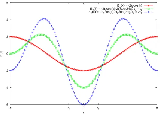
-6 -4 -2 0 2 4 6

π k_F

-k_F 0 -π

E(k)

k

E₁(k) = -2t₁cos(k) E₂(k) = -2t₁cos(k)-2t₂cos(2*k), t₂ = t₁ E₂(k) = -2t₁cos(k)-2t₂cos(2*k), t₂ = 2t₁

Figure 2.1.: The dispersion relation, E(k), of the non-interacting tight binding chain at filling N/L = 0.4. The hopping matrix element t_lm are here restricted to only nearest- neighbour and next-nearest hoppingst_l,l±1=t₁ and t_l,l±2 =t₂, respectively.

Next, we introduce an interatomic distance, i.e. the lattice parameteraand the wave function

|ψ_li (Wannier function) for an electron on an isolated atom located at la. The wave function of an electron on a 1d chain of such atoms is given by

c^†_l|Ωi

z}|{|ψ_li = 1

√L

B.Z.X

k∈[−π/a,π/a]

exp(−ikla)

c^†_k|Ωi

z}|{|ψ_ki, |ψ_ki= 1

√L XL

l=1

exp(ikla)|ψ_li (2.3)

whereLdenotes the total number of atoms in the chain. |ψ_ki(Bloch function) carries a quasi- momentum indexk and makes it possible to calculate the expectation value of the Hamiltonian in the crystal. Here the sum on k runs over the L k−points spanning the Brillouin zone, i.e.

k= 2πm/aLwith integers−L/2< m≤L/2. The field operators associated with the Wannier functions are defined by

c^†_lσ|Ωi

z}|{|ψ_li = Z La

0

dx

c^†σ(x)|Ωi

z}|{|xi hx|ψ_li, (2.4)

i.e.

(15)

c^†_lσ = Z La

0

dx ψ_l(x)c^†_σ(x), c^†_σ(x) = XL

l=1

ψ^?_l(x)c^†_lσ(x). (2.5) In the above equation, the spin degree of freedom is restored. Physically, c^†_lσ can be interpreted as an operator creating an electron with spinσ at sitel. The operatorsc_lσ, andc^†_lσ obey fermionic anticommutation relations

c_lσ, c^†_mσ0

+=δ_σσ⁰δ_lm.

In the presence of a two-body Coulomb interaction, a substitution of the field operators in Eq. (2.) by Wannier operators generates the generalised tight-binding Hamiltonian

H=−X

lm

X

σ

t_lmc^†_lσcmσ +X

lmrs

X

σσ⁰

U_lmrsc^†_lσc^†_mσc_rσ⁰csσ, (2.6) where the hopping matrix elements are given by

t_lm=−hψ_l|H⁰|ψ_mi= 1 L

X

k

e^{−i(l−m)ka}_k=t^?_lm, (2.7) and the interaction parameters are set by

U_lmrs = 1 2

Z La 0

dx Z La

0

dx⁰ψ_l^?(x)ψ_m^? (x⁰) e²

|xˆ_i−xˆ_j|ψr(x⁰)ψs(x). (2.8) Physically t_lm represents the probability for an electron to hop from a site l to a sitem.

In the momentum basis,c_lσ =L^−1/2PB.Z.

k e^−ilkac_kσ, the non-interacting Hamiltonian is di- agonalised asH⁰=P_B.Z.

k c^†_kσc_kσ. Fig 2.1 depicts the cosine band thus obtained.

Let us suppose that the energy of an electron in the state |ψ_li is . If this orbital is highly localized, then the amplitude for it to tunnel or hop between sites will decay exponentially with distance between sites, and to a good approximation, most of the matrix elements of the general tight-binding model are small and can be neglected.

Focusing on the most relevant:

2.2.2. Hubbard model

• Short-Range Coulomb Interactions

How are electronic states in the conduction band modified by the Coulomb interaction (Eq.

2.8) between electrons?

In the atomic limit where the atoms are well-separated and the overlap between neighbouring orbitals is weak, the matrix elements t_lm and U_lmlm are exponentially small in the interatomic separation. By contrast the on-site Coulomb or Hubbard interaction

(16)

X

l

X

σ

U_llllc^†_lσc^†_lσ0c_lσ⁰c_lσ =UX

l

ˆ

n_l↑nˆ_l↓, (2.9)

whereU = 2U_llll, increases as the atomic wavefunctions become more localised.

Therefore, in the atomic limit, a strongly interacting many-body system of electrons can be described to a good approximation by

H=−tX

hlmi

X

σ

c^†_lσc_mσ+Unˆ_l↑nˆ_l↓, (2.10)

where we have introduced the notationhlmito indicate a sum over neighbouring lattice sites, and t=t_lm (assumed real and usually positive). We set the constant energy ₀ =t_ll = 0. The above Hamiltonian has just two parameters: the matrix elementtof an electron jump from one site to an adjacent site in the lattice and the parameterU is the local Coulomb repulsion which operates when two electrons occupy the same orbital. These two forces compete to determine whether a material is conducting or insulating. U must be taken into account when it is not negligible compared to the kinetic energy of the electrons. The kinetic energy to be compared withU is represented by the band widthW = 4t. This is due to the fact that the wave function of the localized electron is composed of a linear combination of theψ_kσ(x) of (2.3). Therefore the energy of the localized electron is represented approximately by the maximum energy, W, available in the tight-binding model.

The model (2.10), proposed in Refs [6, 7, 8], has become known as the Hubbard model.

This is one of the simplest interacting fermionic models one can write and has been extensively studied to describe the theory of strongly correlated electron systems (SCES), for whichU is greater than or of the order of W. In particular, the Hubbard model can explain certain materials known as Mott insulators that are predicted to be conductors in standard band theory models.

The Hubbard model is the prototype of the short-range models and from a mathematical point of view can be regarded as exactly solved for all fillingsρ=N/L. Lieb and Wu were able, using the Bethe-ansatz technique, to give the exact ground-state wavefunction and a scheme for calculating energy and related static quantities [9]. In the Hubbard model, written in the site representation, the Coulomb term is diagonal, whereas in the Fourier representation the kinetic term is diagonal and it corresponds to the band spectrum

ε_k = 2t Xd

α=1

cosk_α, (2.11)

whered is the dimension of space.

The diagonality of one or another term in the Hamiltonian provides an opportunity of devel- oping perturbation theory for two limiting cases: U W and U W. They are sometimes called the limits of weak and strong coupling, respectively. For weak coupling U W, the

(17)

Hubbard interaction can be treated perturbatively within the framework of the Fermi-liquid theory. In the half-filled case (ρ = 1) the density of states is that of a metal. The opposite limiting case when U W corresponds to a strongly correlated system. When a small pa- rameter W/U is used, it is possible to go over from the Hubbard Hamiltonian to the effective Hamiltonian that is known as thet−J model [18], which describes the motion of electrons on a lattice when there is no more than one electron at any one site and the effective exchange interaction between the nearest neighbours is described by

J = 2t²

U . (2.12)

Perturbation theory treatment in terms of the parameterW/U can be developed for thet−J model. In this case the zeroth approximation deals with single-site atomic states, whereas the kinetic term and the effective exchange are regarded formally as perturbations [19]. In the case ρ= 1 the Hamiltonian of thet−Jmodel reduces to the exchange Hamiltonian in the Heisenberg model. In this case charges are frozen and the low energy configurations just correspond to different spin orientations: in a bipartite lattice, the ground state is always a nondegenerate spin singlet and it is expected to show correlations typical of 1d antiferromagnets: hS_lS₀i ∼(−1)^l/l.

Spin excitations are gapless with linear dispersion relation. See Appendix C for more details on the strong coupling limit.

It follows that the Hubbard model describes itinerant magnetism in the weak coupling limit, and localized magnetism in the tight coupling limit when ρ = 1. The intermediate case when U ∼W, is naturally most difficult to deal with, although physically it is the most interesting because it is in this case that the correlation effects leading to a metal-insulator phase transition are manifested most strongly, localised moments appear, and a strong coupling forms between the behaviour of charge carries and magnetic order [6, 20].

• LR Coulomb Interactions

What is expected to occur when the range of the Coulomb repulsion between conduction electrons is not restricted to within each atom but reaches far beyond next neighbours?

In the tight-binding model, the direct termsU_lmml =V_lminvolve integrals over square moduli of Wannier functions and couple density fluctuations at different sites,

X

l6=m

V_lmˆn_lnˆ_m, (2.13)

where ˆn_l=P

σc^†_lσc_lσ. Such terms have the capacity to induce charge density instabilities.

ForV_lm/W 1 (|l−m|<∞), all electrons repel each other. In the case of the short-range repulsion, U, it was meaninful to use the band model because in this case electrons can move freely unless two of them come onto the same atom. In the present case, however,V_lm is larger for two electrons distant from each other than the energy W gainded by a free motion. All electrons will become localized in such a way as to minimize the total Coulomb energy. The

(18)

resultant ordered structure of electrons is called a WL of electrons as was mentioned early in the introduction. The lattice distortion here (due to the charge structure) is driven by electrons which tend to distribute themselves equidistantly.

If W = 0, the system is of an insulating character. When W 6= 0, however small it is compared to V_lm, electrons will more or less be able to move. This is particularly so when the electron density is low and hence the mean distance between neighbouring electrons is long, in which case the movement of an electron to its neighbouring electrons will cause only a small increment in the Coulomb energy.

The open questions regard the effects of doping in the presence of LR repulsive interactions.

In the bare Hubbard model ( short-range interaction), as soon as we insert holes into the lattice, the charge gap closes and both the charge and the spin branch of the excitation spectrum acquire linear dispersion relation, characterized by finite charge and spin velocity, as was shown in [21]

and references therein. In this class of spin isotropic Luttinger liquids, the long wavelength properties of the system are determined by a single dimensionless parameterK_ρ governing the power-law decay of all correlation functions. The antiferromagnetic correlations in the ground state are characterized by the wave vector q = 2k_F and decay as x^(1+K^ρ⁾ while the density correlations are dominated by oscillations at q = 4k_F and behave as x^−4k^F. The analysis based on bosonization technique [22] showed that the LR nature of the Coulomb interaction is expected to change this picture: while the spin sector is unaffected by interactions, the charge spectrum now becomes non analytic: ω_q∼qp

|lnq|. Formally this corresponds to theK_ρ→0 limiting case. In fact, the leading power law behavior of spin correlations is just cos(2kFx)/x while charge correlations decay more slowly than any power law and the momentum distribution is continuous with all its derivatives at the Fermi momentum. Actually, the bosonization study allowed to determine the precise form of the asymptotic behavior, which turns out to be:

<S(x)·S(0)> ∼ exph

−c(lnx)^1/2icos(2k_Fx)

x ,

< n(x)n(0)> ∼ exph

−4c(lnx)^1/2i

cos(4k_Fx),

< c^†_x,σc0,σ > ∼ exph

−c⁰(lnx)^3/2i

cos(kFx), (2.14)

withcandc⁰ non universal positive constants, andkF is the Fermi wave vector and is equal to k_F =ρπ/2.

• Coulomb Interactions and CDW

The investigation of CDW and its influence on the properties of materials has been the subject of intense research for many decades now. Such a phenomenon is often observed in low- dimensional metallic systems, where the spatial modulation of the conduction electron density has a periodicity different from that of the undistorted lattice. As a consequence, a gap opens up in the single-particle excitation spectrum of such materials. Interestingly would be the occurence of CDW in insulators. The conclusion we have reached from the role of Coulomb interactions in the limit where the Coulomb energy is much larger than the band energy is that this can produce a CDW. Thus, a possible origine of CDW in insulators is a large Coulomb

(19)

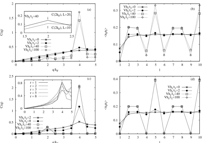
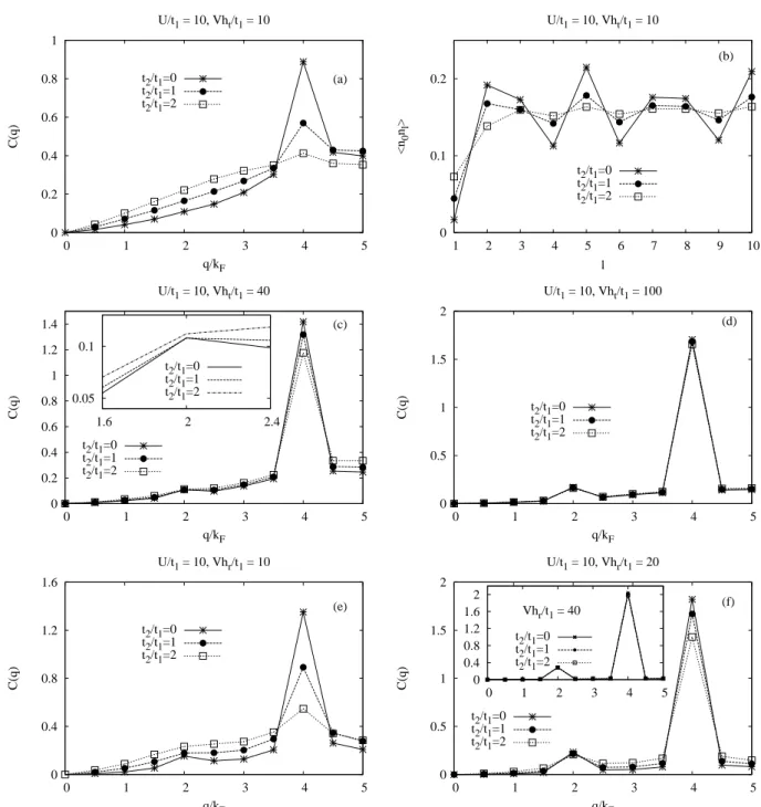
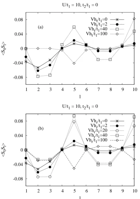
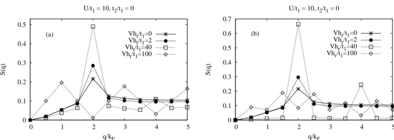
interaction. For instance, as we will show in Chap. 5, at ρ = 0.4, the apparent structure is specified by the wave numbers 2k_F and 4k_F. The apparent 4k_F CDW is the dominating one.

The formation of 2k_F CDW appears only for very large LR Coulomb repulsion. Any material in which both the 2k_F and the 4k_F CDW appear, has two kinds of 1d chain. Therefore a possibility is that one of the two types of chains has a weak interaction among electrons giving rise to the 2k_F CDW while the other, having a strong Coulomb repulsion, brings about a 4k_F CDW.

Another possibility, however, must also be remembered, i.e. that the 2kF and the 4kF CDW may coexist on a single kind of 1d chain [23, 24, 25] which corresponds to our results shown in Chap. 5. In such a case, one of four waves, a 4k_F CDW, and a 2k_F spin-density wave (SDW) will be dominant depending on the relative magnitudes of the hole-hole repulsion and the NNN hopping. The interchain interaction will be not considered in our study.

However, waves other than the dominant type can coexist. Theories have shown that a 2kF

CDW, and a 4k_F SDW can grow in spite of a presence of electron-electron (hole-hole) Coulomb repulsion [23, 24, 25], and that its growth is assisted by the interchain repulsion [23, 24].

2.2.3. Exchange interaction

A second important contribution from (2.8) for intersite interactions derives from the exchange coupling which induces magnetic correlations among the electronic spins. Setting J_ij^F =U_ijij, we obtain

X

l6=m

X

σ

U_lmlmc^†_lσc^†_mσ0c_lσ⁰c_mσ =−2X

l6=m

J_lm^F Sˆ_lSˆ_m+1 4nˆ_lnˆ_m

. (2.15)

Such contributions tend to induce weak ferromagnetic coupling of neighbouring spins (i.e. J_F >

0). Physically, the origin of the coupling is easily understood as deriving from a competition between kinetic and potential energies. By aligning with each other and forming a symmetric spin state, two electrons can reduce their potential energy arising from their mutual Coulomb repulsion. To enforce the antisymmetry of the two-electron state, the orbital wave function would have to vanish at x = x⁰ where the Coulomb potential is largest. This mechanism is familiar from atomic physics where it is manifest as Hund’s rule.

(20)

(21)

3.1. (q 1 d) Sr

14−x

Ca

x

Cu

24

O

41

- a complex system

Although new composite materials M₁₄Cu₂₄O₄₁ (M=La, Sr, Ca, Ba, Y) have been identified [26, 27], their physical properties have drawn much attention of many experimentalists only with the recent discovery of superconductivity in Sr_0.4Ca_13.6Cu₂₄O₄₁, a material heavily doped by Ca, under high pressure [28]. The superconductivity is expected to be driven by the spin-liquid ground state with an energy gap, as theoretically predicted by Dagotto, Riera, and Scalapino [29, 30, 31], in the hole doped even-leg ladder structural elements. According to an optical study [32], the role of Ca substitution, which does not change the formal valence of Cu, was thought to transfer holes from the chain to the ladder. Thus, the superconductivity in this system is considered to be realized when the quasi-one dimensionality of holes on the ladder becomes sufficiently weakened. Most experiments have been made on Sr₁₄Cu₂₄O₄₁ (SCO) that has proved more easy to dope than SrCu₂O₃. M₁₄Cu₂₄O₄₁ can undergo a CDW transition.

3.1.1. Crystallographic structure of q1d Sr14−xCaxCu24O41

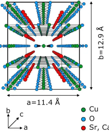
Sr_14−xCa_xCu₂₄O₄₁(SCCO) is built up by alternating layers, edge-sharing CuO₂weakly coupled chains of copper ions which are coupled by the nearly 90^◦ Cu-O-Cu bonds, and two-leg Cu₂O₃ ladders of copper ions, which are coupled by the nearly 180^◦ Cu-O-Cu bonds in the ac plane [26, 27]. Each ladder is coupled by nearly 90^◦ Cu-O-Cu bonds. These two sublayers are separated by (Sr,Ca) atoms and stacked along thebaxis. This structure is denoted in Fig. 3.1.

The chains and ladders run along the c axis and their unit cell parameters roughly differ by a factor of √

2 along this direction, the Cu-Cu distance in the unit cell in the chainscC ≈2.75 ˚A, and in the ladders c_L ≈ 3.9 ˚A. Such a misfit is shown in Fig. 3.2. This misfit leads to an incommensurate modulation of the two sublattices. The lattice constants a and b, which corresponds to the stacking, are the same for both elements.

3.1.2. Electronic structure of q1d Sr14−xCaxCu24O41

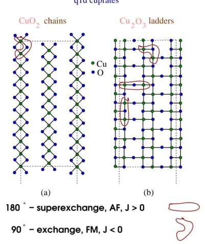
It was shown in [33] and references therein that a superexchange interaction J in insulating cuprates (IC) contains information on the electronic state of these materials and a dependence on the dimensionality of Cu-O network. The compound SCO contains CuO₄ units that are linked to form a variety of Cu-O networks. There are two types of linkage, i.e., the corner- sharing and edge-sharing types, as shown in Fig. 3.3. The former involves the corner sharing of two CuO₄ units forming a straight Cu-O-Cu bond, while the latter type is formed by sharing of the edges of CuO4 units with an almost 90^◦ Cu-O-Cu bond angle. The chains are composed of edge-sharing corners with a very weak ferromagnetic 90^◦ Cu-O-Cu bond whereas the ladders contain both types of linkage. The copper moments are coupled by an almost 180^◦ Cu-O-Cu bond angle. The neighboring ladders are coupled by almost 90^◦ Cu-O-Cu bonds which give a ferromagnetic interaction. Because this ferromagnetic interaction is much weaker than the dominant antiferromagnetic interaction, these ladders are almost decoupled.

(22)

Figure 3.1.: The crystal structure of SCO viewed along the caxis.

Cu O

C

_chain

C

ladder

a

chain

a

ladder

(b) (a)

Figure 3.2.: (a) and (b) show the chain and the ladder of copper ions in SCO, respectively.

The dashed rectangles represent the universal unit cell in the (010) crystallographic plane. Here,c_chain andc_ladderrepresent the CuO₂chain and Cu₂O₃ladder subunits, respectively.

(23)

− superexchange, AF, J > 0

− exchange, FM, J < 0 180

90

Cu O

(b) (a)

q1d cuprates

CuO₂ chains Cu O₂ ₃ladders

Figure 3.3.: Linkage of two CuO₄ units. (a) Corner-sharing and (b) edge-sharing structures.

The electronic structure of the parent compound SCO was calculated ab initio within the local-density approximation [34]. The calculations were performed on a small unit cell con- taining one formula unit of SCO and neglecting the structural modulation. The compound was calculated as a metal, leading to a finite density of states (DOS) at the Fermi energy E_F. However, an insulating behavior was observed for SCO by angle-resolved photoemission spectroscopy (ARPES) experiments. The total DOS is compared with ARPES with fairly good agreement [35]. It was found that the chain bands near E_F are mainly composed of the anti- bonding combination of Cu dxz orbitals and O px and pz orbitals, while the ladder bands are composed of Cud_x2−z² orbitals and Op_xandp_z orbitals. These bands of both subsystems have

180

~ 90 CU

O

(a) (b)

Figure 3.4.: Linkage of two CuO₄ units. (a) Corner-sharing and (b) edge-sharing structures.

(24)

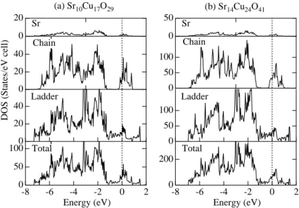
40 20 0

Chain

40 20 0

Ladder

100 50

0-8 -6 -4 -2 0 2

Energy (eV) Total

20 0

Sr

DOS (States/eV cell)

50 0

Sr

200

0-8 -6 -4 -2 0 2

Energy (eV) Total

100 50 0

Ladder 100

50 0

Chain

(a) Sr₁₀Cu₁₇O₂₉ (b) Sr₁₄Cu₂₄O₄₁

Figure 3.5.: The total and partial density of states of (a) Sr₁₀Cu₁₇O₂₉and (b) Sr₁₄Cu₂₄O₄₁. a pseudo-one-dimensional character and the interladder hoppings are 5−20 % of the intraladder ones. In both subsystems, the bands were fitted by simple q1d tight-binding dispersions with NN and NNN hoppings between rungs and adjacent ladders and along and between the chains.

For chains the NNN hoppings,t₂, are largest and twice the nearest-neighbour ones. The total and partial DOS is shown in Fig. 3.5.

3.1.3. Hole distribution

A significant feature of the composite (Sr, Ca, La)₁₄Cu₂₄O₄₁ materials is that they are self- doped. In Sr₁₄Cu₂₄O₄₁the Cu average valence is +2.25, i.e., six holes per formula unit (f.u.) are already doped without any substitution. These holes are generally believed to reside essentially in the chain. Bond-valence-sum (BVS) calculations [36, 37] confirm the concept of self-doping holes and give higher BVS values for holes in the chains. Madelug energy calculations [33]

lead to the same conclusion for x = 0 that all holes are in the chains due to their larger electronegativity, resulting in a hole concentration of about 6/10 per Cu site in the chain. On the experimental side, the resistivity and magnetic measurements on La₆Ca₈Cu₂₄O₄₁, with a pure Cu²⁺valence and thus no holes, as well as on compounds with increasing Sr content for La and a corresponding number of doped holes lead to the conclusion that all doped holes reside on the chains of Sr₁₄Cu₂₄O₄₁ giving a Cu^2.6+valence. Holes enter the structural units with larger O/Cu ratios which are the CuO₂ chains. The ladders remain undoped and magnetically inert due to a large spin gap. The moments in the undoped chains interact weakly, and every hole added creates a nonmagnetic CuO₂ unit and decreases the resistivity [38]. However, neutron scattering experiments [39, 40, 41, 42, 43] and optical investigations [32, 44, 45] point to an arrangement of one hole for every other Cu site of the chain. That means that only 5 out of the 6 doped holes reside in the (CuO₂)₁₀chain subunit of Sr₁₄Cu₂₄O₄₁, and one hole is left for the (Cu2O3)7ladder unit. Polarisation-dependent near-edge x-ray absorption spectroscopy fine structure (NEXAFS) [46] studied hole states on both the chain and ladder sites. The finding is that nonisovalent substitution of Sr²⁺ with La³⁺ (or Y³⁺) reduces the nominal hole count from its full value of six holes per f.u. and that the substitutions of Ca²⁺ for Sr²⁺ leave the nominal

(25)

hole nominal constant. NEXAFS confirms the assumption of [32, 44, 45] that one hole per f.u.

resides in the ladders of x = 0. However, it supports the evidence for weaker redistribution of holes from chains to ladders while stronger redistribution was observed by Osafune et al.

[32]. NEXAFS provides the absolute hole counts in the chains and ladders, while Osafune et al. provide only relative numbers. Studies of the hole/spin patterns within the subsystems provide an additional information on the hole distribution at room temperature, as well as at low temperatures.

3.1.4. Chains subsystem Magnetic susceptibility

The magnetic susceptibility is a bulk observable which should not be able to distinguish between the subsystems. Even though the magnetic properties of (Sr, Ca, La)14Cu24O41 have been studied by susceptibility [39, 38, 47], Carter et al. [38] found that the parent compound La₆Ca₈Cu₂₄O₄₁ showed a temperature dependence of the susceptibility consistent with weakly interacting 10(±0.5) Cu²⁺ spins per f.u., all contributed from the chain site. The Cu²⁺ spins in the ladder were virtually inert below 300 K due to the large spin gap. The spin gap on the ladder for Sr₁₄Cu₂₄O₄₁ is much larger; ∆_ladder = 510±20 K (from the nuclear magnetic resonance (NMR) shift; Magishi et al., [48]). A large spin gap in the ladder of the order of 400K is also observed by Neutron Inelastic Scattering [41, 40] and thermal conductivity measurements [49]. This leads to the conclusion that only spins in chains contribute to the susceptibility of q1d cuprates. The spin ladders have a singlet ground state. And surprisingly the spin chains also exhibit a singlet ground state with a spin gap of 11−12meV [38, 50, 40, 51], while homo- geneous spin chains are known to be gap-less in the spin-channel. The question of the nature of ordering which leads to the spin-gaped state in the chains is still open.

Susceptibility measurements [39, 38] suggested that the spin gap in the chains is due to the formation of weakly interacting spin dimers. They found that a simple AF dimer model gives a good fit to the low temperature part of χ. The AF dimer model is based on organising spins along the chain into isolated antiferromagnetically coupled pairs. The solid line in Fig. 3.6 shows the result of the AF dimer model χ= 2N_D(gµ_B)²/kBT[3 +e^(J/k^B^T⁾] with the number of dimersN_D = 2.0 per formula unit (g= 2.05 along the a direction) and the interdimer exchange J = 130K. The deviation of χfrom the dimer model at high temperatures can be attributed to the contribution from the ladders.

Inelastic neutron scattering (INS) and X-ray diffraction (XRD)

Neutron scattering [53, 54, 40, 43] and X-ray diffraction [52] experiments have revealed a periodic spacing of spin dimers and that the chain dimeric units are formed by NNN spins separated by a hole. Matsuda et al. [54] interpreted the observed spin excitations at low temperatures (T = 8K) with a model where two different types of antiferromagnetically coupled dimers exist, characterised by intradimer spin separation of two chain parameters and four chain parameters, 2c and 4c, respectively. Two independent INS groups [40] and [43] have confirmed from their measurements at low temperatures (T = 5−10 K) the assumption proposed by the authors of Cu NMR [50] that dimers are separated by two holes. Such a picture leads to a chain filling of 6 holes per f.u., that is all the holes located on the chains. Their interpreta- tion was based on a model with only AF dimers. Interdimer distance was found to be three

(26)

Figure 3.6.: Comparison forx= 0, of the experimentally measured temperature dependence of the magnetic susceptibility, χ, represented by solid dots, Motoyama et al [47], and the dimer model,N_D = 2.0 per formula unit, indicated by a line.

3 c

2 c 2 c 2 c 3 c 2 c

Figure 3.7.: Structure and periodicity of the spin dimers (framed) with the complementary charge-order of the holes (Zhang-Rice singlet sites denoted by yellow squares) for x = 0 chains in the alternation models. The upper and intermediate models, periodicity 5c, chains hole count 6, are proposed by INS measurements [40], [43], and [42] at 5−20 K. The lower model, periodicity 4c, chains hole count 5, is resulting from XRD measurements [52] at 50K, and INS measurements [42].

(27)

chain parameters, 3c, Fig. 3.7. The chain superstructure periodicity in this model is 5c. XRD results for Sr₁₄Cu₂₄O₄₁ directly point to structural change related to charge-order [52]. These measurements were performed at (T = 50 K). The observed periodicity was equal to 4 chain parameters. This result leads to the choice of the model with the chain hole count 5, Fig. 3.7.

In this model 2.5 AF dimers would appear per 10 Cu sites. We note again the contradiction between the observed charge-order (by XRD) and spin order (by INS) due to different hole counts. However the INS experiments were performed at lower temperatures than XRD.

NMR

NMR offers the possibility of a direct determination of the spin gap. ⁶³Cu NMR signals for the ladder site can be separated from those for the chain site, since nuclei of these sites possess different quadrupole coupling. Kumagaiet al. [55] investigated Sr_14−xCa_xCu₂₄O₄₁by Cu NMR and nuclear quadrupole resonance (NQR). The energy gaps in the spin excitation spectra (spin gap) were confirmed to be ∆ = 140 K for the CuO₂ chain and ∆ = 470 K for the Cu₂O₃ ladder in Sr₁₄Cu₂₄O₄₁. Also they found that the spin gap for the chain is nearly independent of the substitution of Ca up to (x= 9), Y up to (x= 2), and La up to (x= 1). Detailed NMR and NQR studies reveal static distribution of holes below 200 K forx = 0 [50]. Two distinct resonance spectra are obtained for the chain sites. They are assigned to the magnetic Cu sites with spin-1/2 and the nonmagnetic Cu sites. The suggested model to explain these results is that the dimers are separated by at least two nonmagnetic sites, which is in accordance and reproduces the same spin-pattern as deduced from INS.

ESR

Electron spin resonance (ESR) has been studied as a function of temperature and Ca concentration (x= 0−12) [56]. Since the spin ladders show a large spin gap of about 400−500K, the dominant contribution to the ESR signal below 300 K is attributed to the CuO₂ spin-1/2 chains. For all values of x the data reveal a remarkable influence of the hole dynamics on the Cu-spin relaxation. This enables to identify the onset of charge order in the chains for x = 0 and 2 at 200 and 170 K, respectively. A further increase of x rapidly destroys the charge ordered state. A transition to an antiferromagnetically ordered state is observed at 2.5 K for x = 12. The whole set of ESR data can be understood in terms of a transfer of only a small amount of holes from the chains to the ladders with increasing x in Sr_14−xCa_xCu₂₄O₄₁ and a simultaneous crossover from independent dimers to antiferromagnetically coupled chains, which order at low temperatures due to weak interchain interactions.

(28)

(29)

4.1. Introduction

Numerical methods are essential in the investigation of strongly correlated fermion systems, because in such a sysems the perturbation theory to treat the electronic correlations often breaks down. These methods are playing an important role in understanding of how correlation effects determine the properties of strongly interacting electrons. The dimensions of the matrices involved are usually very large and a large number of eigenvalues and their corresponding eigenvectors are needed to compute the desired physical quantities. This presents a problem in numerical treatments and makes it one of the grand challenges in the field of supercomputing. The following chapter will be devoted to the numerical technique based on the Lanczos algorithm. However, the focus will be on the specific area of strongly correlated models, namely 1d fermionic systems, to illustrate various technical aspects of the method and to discuss the physics of these systems.

4.2. Basic idea

ED has played a very important role in understanding the ground state properties of quantum systems. The idea is to set up the Hamiltonian N_H ×N_H matrix for the model in a finite Hilbert space of dimension N_H and calculate the eigenpairs (eigenvalues and eigenvectors) by diagonalizing the matrix. Since the Hilbert space of quantum system grows exponentially with system size, a direct numerical attack is impractical for large N_H as the matrix increases like N_H² and the CPU-time like N_H³. Instead, an iterative scheme known as the Lanczos algorithm [57, 58] is often used to construct iteratively a sequence of orthonormal vectors that form a basis under which the Hamiltonian is real and tri-diagonal [58, 59]. Once in this form the ground state and the low-lying excitation spectrum for small systems (of up to about 10⁸ states) can be found with high accuracy using standard library subroutines [60]. This is especially important for fermion systems where quantum Monte carlo methods suffer from the well known

”negative sign problem” [61]. The Lanczos algorithm is a recursive algorithm. The success of this method is due to the rapidly growing power of supercomputers. The disavantage of ED is that it inevitably suffers from finite size effects. Because of the restrictions on the cluster size, there are limitations for a complete finite-size scaling analysis with this technique (Hilbert space can be dramatically reduced once the symmetry properties are used). Nevertheless, ED is very valuable in supplementing analytical and other numerical results. The Hamiltonian matrices for most quantum spin models are sparse (which is the case of an overdoped system). Although the matrix can be stored in sparse matrix form in the Lanczos iteration, the size of the matrix grows so rapidly with the system size that one may not have enough memory or disk space to store it even as a sparse matrix. The algorithm presented here will be illustrated by considering the example of a Hubbard chain, but it can be applied to any quantum Hamiltonian.

(30)

4.3. The Lanczos method

4.3.1. Invariant subspace

The concept of an invariant subspace is an important point for understanding the Lanczos method. Linear algebra tells us that a subspace that is spanned bymlinear independent vectors

|φ1i, . . . ,|φmiis invariant under a hermitian matrixH, if for any vector |φiin the subspace the vector H|φi is also in the subspace. In the following we will denote the H-invariant subspace by H. What does this invariance mean? If Q_m is a n×m matrix whose columns are the orthonormal vectors|φ_li, then the matrix productHQ_m is an×mmatrix too and the columns are linear combinations of the columns of Q_m. Assuming that the |φ_li form an orthonormal basis in the invariant subspace, i.e. Q^t_mQ_m = id_m, one can find a m×m matrix T_m which satisfies the relation

HQ_m=Q_mT_m⇔Q^t_mHQ_m =T_m. (4.1) This means that the eigenpairs of a large matrix H can be found from those of a smaller matrixT_m. For instance, let λand |vi be an eigenpair of T_m. Multiplication of T_m|vi= λ|vi byQ_m and the use of relation (4.1) leads to the equivalence

4.3.2. The algorithm

Following is a brief idea about the steps involved during the construction of the H-invariant subspaceH.

First step: the initial state

In this procedure it is necessary to select an arbitrary but nonzero normalized vector |φ₀i (hφ₀|φ₀i= 1) which belongs to the Hilbert space Hof the model being studied. If some information about the ground state is known, like total momentum or spin, then it is convenient to start the iteration with a vector already belonging to the subspace having those quantum numbers. Otherwise, it is convenient to select an initial vector with randomly chosen coefficients.

Second step: orthogonality

After|φ₀iis selected, a second normalized vector |φ₁ican be constructed by multiplying the hermitian matrixH with the initial vector

b₁|φ₁i=H|φ₀i −a₀|φ₀i. (4.3)

(31)

To ensure the orthogonality hφ₀|φ₁i = 0 one has to subtract the projection onto |φ₀i. One imposes

a₀ =hφ₀|H|φ₀i, (4.5)

that is a0 is the average energy of |φ0i. In addition, b1 can be found by taking the scalar product of Eq. (4.3) withhφ₁|

b1 =hφ1|H|φ0i. (4.6)

Notice that, by using Eq. (4.3), one also has that

b²₁ =hφ₀|(H −a₀)(H −a₀)|φ₀i=hφ₀|H²|φ₀i −a²₀, (4.7) that is b₁ is the mean square energy deviation of |φ₀i.

By repeating the above procedure, we define the third normalized vector, in such a way that it is orthogonal both to |φ₀i and |φ₁i

b₂|φ₂i=H|φ₁i −a₁|φ₁i −b|φ₀i. (4.8) The conditions of orthogonality are

hφ₁|φ₂i= 0⇔a₁ =hφ₁|H|φ₁i, (4.9)

hφ₀|φ₂i= 0⇔ hφ₀|H|φ₁i −b= 0⇔b=b₁, (4.10) and finally, the fact that |φ₂iis normalized leads to

b₂ =hφ₂|H|φ₂i. (4.11)

This procedure can be generalized by defining an orthogonal basis recursively. Suppose one has constructed the Lanczos vector up to |φm−1i

b_m−1|φ_m−1i=H|φ_m−2i −a_m−2|φ_m−2i −b_m−2|φ_m−3i, (4.12) with

(32)

am−2 =hφm−2|H|φm−2i, b_m−2 =hφ_m−2|H|φ_m−3i, b_m−1 =hφ_m−1|H|φ_m−2i.

(4.13)

orthogonal to all|φ_jiwithj ≤m−2. Then one defines

b_m|φ_mi=H|φ_m−1i −a_m−1|φ_m−1i −b⁰|φ_m−2i −

m−3X

j=1

A_j|φ_ji. (4.14) The conditions of orthogonality reads as

hφ_m−1|φ_m−1i ⇔ia_m−1 =hφ_m−1|H|φ_m−1i,

hφ_m−2|φ_m−1i ⇔b⁰ =hφ_m−2|H|φ_m−1i=b_m−1, A_j =hφ_j|H|φ_m−1i,

(4.15)

but, because one has

b_j+1|φ_j+1i=H|φ_ji −a_j|φ_ji −b_j|φ_j−1i, (4.16) and j+ 1≤m−2, one obtains that

A_j = 0. (4.17)

Then,|φ_mi, once orthogonalized to|φ_m−1i and |φ_m−2i, it is automatically orthogonal to all the previous vectors.

Thus, at each Lanczos step, it is sufficient to orthogonalize only to the previous two vectors, and the orthogonality with the previous ones is automatic. That makes the Lanczos algorithm very efficient.

After j =m steps a set of orthonormal vectors |φ_mi has been generated. These vectors are the columns of an orthonormal matrixQ_m. By applying formula (4.1) the Hamiltonian matrix H will be transformed into a tridiagonal symmetric matrix, whith a_j on the diagonal and b_j below and above the diagonal

Q^t_mHQ_m =T_m=







a₀ b₁ 0 0 . . b₁ a₁ b₂ 0 . . 0 b₂ a₂ b₃ . . 0 0 b₃ a₃ . .

. . . .







(4.18)

(33)

Ifmis sufficiently large, the eigenvaluesλof the Lanczos matrixT_m should be good approx- imations of the eigenvalues of Hwhich are restricted to the invariant subspace

H= Spann

|φ₀i,H|φ₀i,H²|φ₀i, . . . ,H^m−1|φ₀io

, (4.19)

known as Krylov subspace generated by application of H to |φ₀i. In practice for large systems, the iterations will stop at a much earlier stage. Either after some Lanczos iteration steps n_L (typically of the order of ∼ 100 steps), or when b²_j is smaller than a chosen preci- sion value. For instance for Hubbard model with 10 sites and periodic boundary conditions at a densityρ= 0.4 and zero magnetization, the termination is signaled ifb²_j is smaller than 10⁻¹³. The main aim in the numerical realization of the Lanczos algorithm is to keep computational effort low. The most expensive operation is the matrix-vector multiplication H|φ₀i. In addition, the Hamiltonian matrix cannot be stored in the computer memory. The storage of matrix elements would require too much memory. With the Lanczos algorithm, one needs only two or three vectors of dimensionN_H (two vectors are enough for making the Lanczos procedure).

When we are interested in having the ground-state vector, and not only the eigenvalues, three vectors are useful to avoid a lot of writing and reading from the hard disk.

4.4. Application of the method: Hamiltonian of the model

As an example we will sketch how to implement the Lanczos method for the 1d one-band Hubbard model with nearest neighbor hopping tand local Coulomb repulsion U

H=−t X

<ij>,σ

c^†_iσc_jσ+H.c.

+UX

i

n_i↑n_i↓. (4.20)

The Hamiltonian is applied to a chain with 20 sites and periodic boundary conditions.

The possible configurations of up-spins are independent of the configurations of the down spins and the Hilbert space HHubbard of all possible configurations is just the direct product of the Hilbert space of down spins H↓ and of up-spinsH↑

HHubbard =H↓⊗ H↑. (4.21)

In order to actually be able to express the Hamiltonian as a matrix, we need a basis of the Hilbert space. Since the model’s Hamiltonian conserves the total electron number and the electrons’ z-component S_z of the total magnetization, we can restrict ourself to the subspace whose basis states have a certain number of up and down spins. We thus want to construct a basis of all states withN particles onL sites and a givenS_z. Each basis state of this subspace is identified by an indexα between 1 and the subspace dimension

dim=

L!

N_↑! (L−N_↑)!

L!

N_↓! (L−N_↓)!

. (4.22)

(34)

By doing so, we generate two lists, the ”small” list called ’basis’ gives the occupation index α for each basis state index. The ”big” list called ’Hspace’ (total Hilbert space) gives the basis state index for a given occupation index α (or −1 if α corresponds to a state with wrong quantum numbers). The advantage of this representationis, that, except for the special case of a system with only up spins or only down spins, these two spaces are much smaller that the total Hilbert space. Therefore it is possible to keep an inverse list of all bit patterns for the up and down spins in memory. And the search for the index of a new configuration reduces to two lookups in these tables to find the up-index and the down-index. An implementation for the two-dimensional Hubbard model, using this representation, is described in detail in Ref.

[62]. For instance, if we restrict ourself to the subspace with zero magnetization and a density n= 0.4, the Hibert space thus has dimension

20 4

2

'23 million, whereis the dimension of the total Hilbert space is 4²⁰.

The occupation number basis for a system of Lsites is defined as

|ni=|n_1↑n_1↓n_2↑....n_L−1↓n_L↑n_L↓i= Y

iσ,niσ=1

C_iσ^† |0i, (4.23) where|0i is the vacuum state. The occupation indexα is defined as

α= XL

i=1

n_i↑2²ⁱ⁻²+n_i↓2²ⁱ⁻¹

. (4.24)

The many-body Hamilton-matrices are sparse. Only a small fraction of all matrix elements is not zero. And since we are interested in low density n= 0.4, the matrix is very sparse, it is then practical to store only the nonzero matrix elements not only to save memory but also to speed up operations of the formH|vi which form the heart of the ED procedure.

See Appendix A for more details about coding the basis states.

4.5. Symmetry operations: reducing Hilbert space dimension

The Lanczos method gives essentially exact results for ground-state and low lying eigenvectors.

In spite of these advantages, memory limitations impose severe restrictions on the size of the clusters that can be studied within this method. This problem can be considerably alleviated using the symmetries of the Hamiltonian that reduce the matrix Hamiltonian to a block form.

We have already used two symmetries, the conservation of particle number and the conservation of the z−component of the total magnetisation. To reduce further the sise of the matrix, we considere as well the momentum conservation due to translational invariant in systems with periodic boundary conditions. The total number of basis states is greatly reduced byL lattice translations with lattice displacementsR_l, l= 0,1,2, . . . , L−1,. The average reduction is∼1/L.

The total number of basis states is now about 1 million forρ= 0.4, andL= 20. Let us define the lattice translation operator T_l, l = 0, . . . , L−1, which bring site ito site T_l(i) through the relation