1Introduction 1.1The Atmospheric Boundary Layer

- 1 -

1 Introduction

1.1 The Atmospheric Boundary Layer

The Atmospheric Boundary Layer (ABL) constitutes the lower boundary of the atmosphere towards the surface and this is obviously the basis for its name.

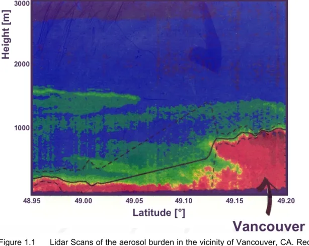
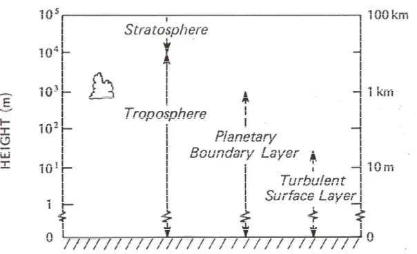
The homogeneous atmosphere has a depth of roughly 100km, its lowest portion, the Troposphere, is on the order of 10km deep and the lowest roughly 1000m of the latter are called Atmospheric Boundary Layer, Planetary Boundary Layer or sometimes simply Boundary Layer (Fig. 1.2). Hence, the ABL covers only the lowest about one percent of the atmosphere if we count in meters. In terms of mass, however, this translates into something like 20%, when considering the exponential decrease of pressure with height. Still, this substantial fraction of atmospheric mass is not the only reason why the Atmospheric Boundary Layer is often treated as a separate entity in textbooks and even university curricula. Its name does not only refer to its location, but also reflects the fact that the proximity of the Earth’s surface has a profound influence on the flow characteristics within the ABL (Fig. 1.1).

Figure 1.1 Lidar Scans of the aerosol burden in the vicinity of Vancouver, CA. Red

colour stands for a high aerosol concentration, blue for low. Solid and

dashed lines estimates of the boundary layer thickness and

entrainment zone, respectively. Flow from the west. The figure shows

the influence of the sea-air transition on the boundary layer structure

and depth. From Hägeli (1998).

First of all, the atmospheric flow, which is forced by the large-scale pressure distribution, is subject to surface friction. This introduces strong gradients in mean wind speed close to the ground. Second, atmospheric radiation strongly interacts with the surface. Due to different thermal properties of the surface material and the near-surface air, absorption (all wave lengths) and emission (essentially long-wave radiation) lead to large gradients in temperature near the ground. Both these processes, friction and surface radiative energy exchange through the introduction of gradients make the flow unstable at small scales and hence prone to turbulence. In fact – as we shall see in Chapter 2 – the conditions in the ABL are almost always and almost everywhere such that the flow is turbulent. Moreover, very often it is dominated by turbulence. Hence, a suitable definition of the Atmospheric Boundary Layer is to state that the ABL is the lowest distinct layer of the atmosphere next to the Earth’s surface wherein the flow is characterised by turbulence.

Surface friction (mechanical turbulence) is always a source for turbulence near the ground. Energy exchange through radiation (thermal turbulence), on the other hand may either increase turbulence or act towards damping it.

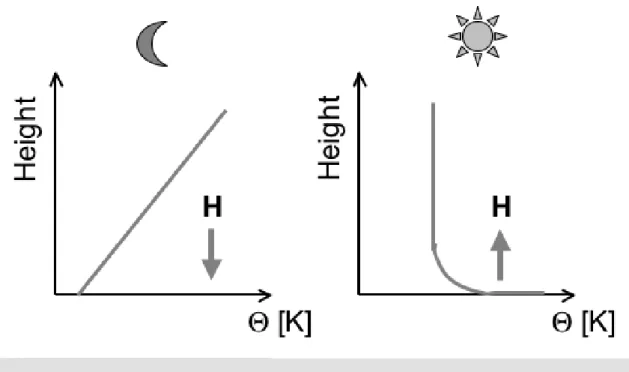
Although we will look at this in detail only in Chapter 6, it is instructive to consider here two very simple cases. During the day, the surface radiation balance is positive (Section 1.3) thus heating up the ground (Fig. 1.3). An air parcel that is displaced vertically away from the ground will find itself being warmer than the surroundings and continues to rise. This is an unstable stratification that supports production of thermal turbulence. Frictional plus thermal turbulence production then lead to a strongly turbulent boundary layer, which has a considerable vertical extension. On the other hand, if the ground cools during the night due to a negative radiation balance, a vertically displaced parcel is colder than its environment and the initial vertical movement is damped. This is called a stable stratification, turbulence is correspondingly weak and the boundary layer is shallow. A common measure for this static stability is the vertical gradient of the potential temperature, viz.

€

θ = T p

p



  

 

κ

, (1.1)

where T is the temperature, p the pressure, p

the reference pressure (1000 hPa) and

€

κ = 0.286 . A positive gradient in

€

θ corresponds to a stable

stratification, and vice versa for unstable stratification. The idealized state in

between is called neutral. In Chapter 6 we will see how static stability is

related to more general stability measures that take into account the

turbulence state of the flow (dynamic stability).

- 3 -

Figure 1.2 The vertical structure of the homogeneous ABL.

An important property of turbulent flows is that they can transport momentum, energy and mass without a mean velocity component in the respective co- ordinate direction. In the ABL the dominant direction of turbulent transport is the vertical due to the strong vertical gradients close to the surface. Hence, the turbulent nature of the ABL flow is responsible for an effective exchange of momentum, sensible heat, water vapour and other trace constituents such as pollutants from and to the surface. The transport of water vapour, in particular, means that the content of every raindrop has earlier been subject to turbulent transport when leaving the Earth’s surface and thus emphasises the importance of this process for atmospheric processes on all scales.

Moreover, transporting water vapour also means transporting a form of

energy, namely the energy that is necessary for evaporation, which is later

and elsewhere released when condensation takes place. Therefore, transport

of humidity is often referred to as transport of latent heat.

Figure1.3 Profiles of potential temperature and direction of sensible heat flux during the night (left) and during the day (right).

Table 1.1 summarises the basic properties of the ABL for unstable, neutral and stable stratification.

Stratifi-

cation Turbulence Vertical extension

Sensible heat transport

€

∂θ / ∂ z ^Occurrence

Stable + Mechanical – thermal

Shallow [O (200 m) ]

Down > 0 Night, snow, ice cover Neutral + Mechanical Medium

[O (1000 m) ]

Nil 0 Strong wind

(idealised) Unstable + Mechanical

+ thermal

High

[O (1-2 km)]

Upward < 0 Day

Table 1.1 Basic properties of idealised states of the ABL. Column ‘turbulence’

refers to turbulence production (+) and suppression (-), respectively.

Over ideal horizontally homogeneous surfaces turbulent transport is solely in

the vertical and at the same time it constitutes the dominant mechanism of

vertical transport for many entities. It is equalled in importance only by the flux

of radiative energy in both the long and short wave ranges. This ideal type of

boundary layers is covered in Part I of this book. A physical description of

turbulent transport will be given in Chapter 3. In the remainder of the present

- 5 -

chapter we simply keep in mind that it exists and look at some of its characteristics.

Over real and in general non-homogeneous surfaces transport with the mean flow (advection) becomes important as well. Still, close to the surface the mean vertical wind component vanishes and turbulent transport is responsible for large parts of the vertical exchange. In Part II, we will look at a number of problems related to this type of ABLs.

1.2 Phenomenological Overview

1.2.1 The ideal neutral boundary layer

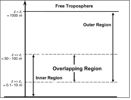
This type of boundary layers is best investigated, mainly from laboratory flows and applications of industrial Fluid Dynamics. Although its premises (stationarity, horizontal homogeneity, strictly neutral stratification) almost never apply in the real atmosphere, it is instructive to have a look at its properties and the concepts applied. Basically, we can distinguish two different regions according to the main factors influencing the flow (Fig. 1.4):

Figure 1.4 Schematic representation of the ideal neutral ABL. Here

€

z

denotes the ABL height and

€

z

the roughness length (see Chapter 4, eq. 4.16).

Inner Region:

• Lowest distinct layer of the atmosphere

• The structure of the flow is determined by surface friction

• Acceleration due to the Earth’s rotation (Coriolis acceleration) can safely be neglected

• The dominant length scales are the distance from the surface (i.e., height z and the typical dimension of the roughness elements,

€

z

)

• Turbulent fluxes do not significantly vary with height if not too close to the surface (see below)

Outer Region:

• The influence of friction decreases with height, while acceleration due to Coriolis effects increases

• Its upper boundary constitutes the transition to the (quasi-) Geostrophic equilibrium between acceleration due to pressure force and Coriolis effect.

• The dominant length scales are the height of the boundary layer,

€

z

, and again the height z.

• Turbulent fluxes are variable with height, essentially decreasing to zero at its upper boundary.

These two regions do not have sharp boundaries so that we can consider an overlapping region in between (Fig. 1.4). Due to the importance of scaling arguments in boundary layer meteorology (Chapter 4) we look at a theoretical prediction for the profile of mean wind speed,

€

u , in this overlapping region.

We start with noting that we have three length scales,

€

z ,

€

z

and

€

z

that can be combined to form two non-dimensional ratios:

€

z / z

and

€

z / z

. If we express the gradient of mean wind speed in a non-dimensional form it must be a function of these two ratios alone

:

€

∂u

∂z z

u

= φ( z z

, z

z

) (1.2)

Here, we have introduced a scaling velocity,

€

u

which for the time being can be regarded as a typical velocity for the neutral boundary layer. We will later (Chapter 3) come back to its definition and will call it friction velocity.

€

φ ^{is a} non-dimensional (universal) function with the given arguments and its functional form is of no importance for the moment.

In the Inner Region, the wind profile will by definition not be dependent on

€

z

, hence

€

z/

lim

φ ( z z

, z

z

) = φ

( z

z

) . (1.3)

In the Outer Region, on the other hand,

€

z

will be unimportant and thus

€

z/z_s→∞

lim φ ( z z

, z

z

) = φ

( z

z

) . (1.4)

If there is a matching layer, in which both properties apply we must have

€

φ

( z

z

) = φ

( z

z

) : matching layer, (1.5)

1 In chapter 4 we will address some more stringent conditions on how to choose and determine a complete set of relevant variables.

- 7 -

and this is only possible if both non-dimensional functions approach a constant value:

€

z/z_i→0 z/z_s→∞

lim ( ∂ u

∂ z z

u

) = const. (1.6)

Integrating between two levels

€

z

and

€

z

after separating the variables yields

€

u (z

) − u (z

) = const. u

ln( z

z

) . (1.7)

If we, finally, define the lower level as the one at which the mean wind speed vanishes (

€

u (z

) ≡ 0 ) and denote the constant with 1/k (we will later learn that k is the v. Kàrmàn constant) we finally have the logarithmic profile for the matching layer:

€

u (z) = u

k ln( z

z

) (1.8)

This logarithmic behaviour is indeed often observed close to the surface under near-neutral conditions.

A word is in order concerning names. The Outer Region is in the atmospheric context often called Ekman Layer. Its properties will be investigated in more detail in Chapter 5. The Inner Region is often referred to as the Surface Layer (SL) but this is at least problematic and only justified due to the origin of this name. In laboratory flows with small roughness elements (small

€

z

as for sand grains, microscopic elements of the surface, etc.) the lowest measurable layer has in fact the properties of the matching layer and the logarithmic wind profile can usually be observed down to the lowest measured level. Therefore, the description of the flow in this layer is often referred to as surface layer scaling.

However, over real surfaces with roughness elements such as plants, rocks or

even buildings, there is a distinct layer below the logarithmic layer. Therefore,

in principle the Inner Region has to be considered in two parts (Tennekes and

Lumley 1972): The true matching region is called Inertial Sublayer (IS) and

here the log-profile and other predictions of so-called surface-layer scaling (or

Monin–Obukhov Similarity Theory, MOST, see Chapter 4) apply. Below, there

is a layer wherein the flow is directly influenced by the three-dimensional

structure of the roughness elements: the Roughness Sublayer (RS). We shall

turn to this layer in more detail in Section 8.2. So we face the problem that

what is generally referred to as surface layer scaling applies only in the IS,

while the lowest layer next to the surface is called Roughness Sublayer and

there, surface layer scaling does not apply. Still, we will use the widely used

term Surface Layer for the lowest portion of the ABL throughout this book and

only make the appropriate distinction where necessary.

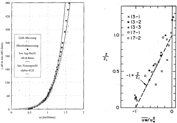
Figure 1.5 Typical Profiles in the neutral ABL. Left: profile of mean wind speed (‘logarithmic profile’) from wind tunnel observations of Kastner-Klein (1999). Scaled with observation at 60mm; right: profile of momentum flux (

€

u' w'

) scaled with the characteristic velocity

€

u_*

throughout the entire near-neutral ABL (from Brost et al. 1985).

Figure 1.4 depicts typical profiles in near-neutral conditions. The turbulent flux of sensible heat vanishes by definition while the profile of momentum flux reflects the forcing at the ground and decreases linearly with height. Mean wind speed is characterised by the logarithmic behaviour close to the ground and an increases towards the ABL top. This latter is – due to a uniform temperature profile - not very well defined and is sometimes deduced as the height where Geostrophic equilibrium is first reached. We will come back to explicit semi-empirical formulations later.

1.2.2 The convective boundary layer

The Convective Boundary Layer (CBL) is characterised by a three-layer structure (Fig. 1.6). Close to the surface (lowest 10%) the unstable SL exhibits a strong decrease in potential temperature away from the heated surface. The strong turbulence, mechanical plus thermal in origin, leads to large eddies (on the order of the ABL height

€

z

) and strong vertical mixing. Therefore, the middle about 80% of the CBL is well-mixed and essentially no gradients are present for mean variables. This gives rise to its name Mixed Layer (ML).

Note that the CBL or unstable boundary layer has, despite of its name, a uniform

€

θ -profile except close to the surface. Under ideal circumstances the

CBL is topped by an entrainment layer that is characterised through a usually

strong inversion. The top of the CBL is somewhat arbitrarily assigned here to

the middle of this inversion layer (often, the top or bottom of the latter can be

- 9 -

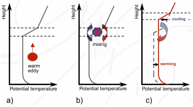
found in the literature, too). The height of this entrainment layer grows during a sunny day as sketched in Fig. 1.5. Warm eddies rise from the unstably stratified SL and continue to do so until they reach the inversion. Due to their kinetic energy the can enter the inversion layer and eventually mix with their new environment. This brings potentially warmer air from the free Troposphere into the CBL with a compensating export of relatively cool BL air.

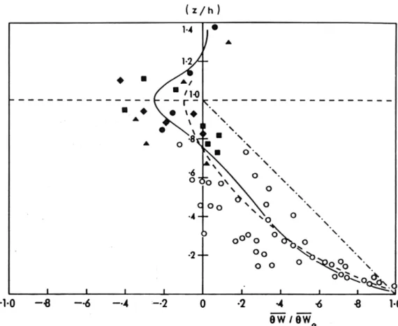
Thus the CBL is not only heated by radiative exchange at the surface but also due to entrainment at its top as it can be seen from the profile of turbulent heat flux, H (Fig. 1.6). The downward entrainment heat flux at the top amounts to about 20% of the surface value. This interaction between surface forcing and entrainment makes it difficult, if not impossible, to diagnose the height of the CBL from easily accessible surface variables. Figure 1.7 shows a typical daily cycle of H with its maximum after solar noon along with the development of the inversion height. Clearly, for equal strength of H (at 10 and 17 CDT, say – see Fig. 1.8) quite different values for

€

z

are present.

Hence, for the determination of

€

z

at a specific time of the day, the ‘history’ of the entire day since sunrise is required (see section 15.1 in connection with air pollution modelling).

Figure 1.6 Schematic of the entrainment process, a) rising of an eddy, b) mixing in the Entrainment Layer and c) resulting temperature profile.

As already mentioned, the strong turbulence in the CBL leads to the formation of big eddies. Relatively strong updrafts [ O (1ms

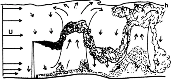
) ] cover about 30-40% of the area while weaker downdrafts (subsidence) prevail in the rest of the domain due to mass conservation (Fig. 1.9). Hence, the vertical velocity component is not normally distributed, but rather (positively) skewed with a slightly negative median (see below, Fig. 3.2). This skewness is strongest at

€

z / z

≈ 0.3 and

plays an important role for air pollution modelling in the CBL (Chapter 13).

Figure 1.7 CBL profile of turbulent heat flux. Data from various experiments. The lines indicate a simple linear profile (dash-dot), and results from numerical simulations. From Caughey (1982).

Figure 1.8 Typical daytime cycle of the surface heat flux (left scale, dots; in

kinematic units) and the height of the ‘mixed layer’ (right scale, denoted

as ‘inversion base’). Form Wyngaard (1988).

- 11 - 1.2.3 The stable boundary layer

Vertical movement of air parcels is reduced or sometimes even completely suppressed due to the stable stratification (Fig. 1.10). Therefore turbulence is only substantial within the SL and becomes weak and rather ineffective higher up. Only small, local eddies contribute to the turbulent transport that decreases faster than linear with height (Fig. 1.11). This situation, in concert with the thermal wind relation can sometimes lead to the formation of a wind speed maximum close to the ground, a so-called low level jet (Fig. 1.10).

The height of the Stable Boundary Layer (SBL) is not very well defined due to the graduate blending of the surface inversion into an often weakly stratified higher layer (cf. Fig. 1.10). Many different definitions for

€

z

under stable stratification, which are not based on the temperature profile, exist. They are, however, often hampered in their practical application due to measurement uncertainties (large relative errors for small variables) or difficulties (requirement to measure a profile up to

€

z

).

The SBL and its turbulence state plays a crucial role in air pollution modelling.

Because turbulent exchange is often weak and the SBL is therefore shallow, concentrations are often high close to the source (generally: close to the ground) and remain so far downstream. Worst-case scenarios usually pick the most stable stratification with the associated most shallow SBL to establish highest possible concentrations. However, the weak turbulence also means that defining variables (turbulent fluxes) are often small and difficult to measure or infer. Understanding aspects of the SBL even over ideally homogeneous surfaces therefore remains an issue of current research, even if the ideal, classical boundary layer is thought to be quite well understood at present.

Figure 1.9 Updrafts and downdrafts in a schematic CBL exemplified in their effect

on air pollutant dispersion from a stack (from Briggs 1988). Updrafts

are stronger and occupy only about 40% of the domain. Thus

downdrafts are generally weaker and more frequent as can be seen

from the pdf (see Fig. 3.2). From Briggs (1988).

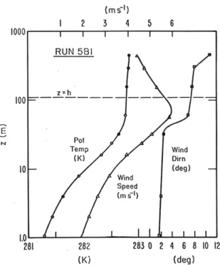
Figure 1.10 Profiles of mean wind speed (triangles) wind direction (squares) and potential temperature (circles) in a stable boundary layer. From Caughey (1982).

Figure 1.11 Profile of local momentum flux scaled with the surface friction velocity

over a ‘permanently’ cold surface on the Greenland ice sheet (from

Forrer and Rotach, 1997). Dashed line: prediction of Nieuwstadt

(1984)

.

- 13 -

1.3 Daily cycle

In the previous section we have seen that the turbulence state of the ABL and hence its vertical extension is strongly dependent on stability. Therefore, it has a pronounced daily cycle, which in turn follows that of net radiation at the surface. Under ideally homogeneous and stationary conditions, the surplus or deficit of radiative energy at the Earth’s surface, is described through the energy balance equation that reads in a simplified form (Rotach and Calanca 2002):

€

NR = H + L

E + G + Δ S . (1.9)

Here, NR denotes the net radiation, H and L

E are the turbulent fluxes o f sensible and latent heat, respectively and G is the ground heat flux. If the energy balance is set up for a volume instead of an infinitesimally thin surface such as the entire canopy layer, a storage term Δ S needs to be included in Equation (1.9). This latter term is the result of a discernible divergence of the other energy fluxes involved and leads to warming or cooling (drying or moistening) of the volume considered.

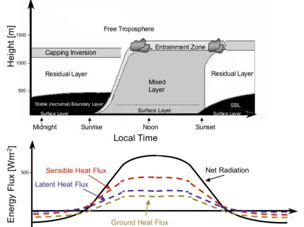
Figure 1.12 Daily cycle of the idealised structure of the ABL (upper panel, modified after Stull 1988) and typical energy balance components (lower panel).

During the day, the net radiation is large and positive leading to the heating of

the surface, positive sensible heat flux and the associated well-mixed deep

CBL (Fig. 1.12). Boundary layer clouds may develop at its top with usually

little to no associated rain or even significant shadowing. Around sunset the surface starts to loose energy due to a negative radiation balance and from the surface a stable nocturnal boundary layer starts to grow. Due to the relatively weak turbulence activity its growth is slow and it reaches a height of only a few hundred meters. It is topped by what is referred to as the Residual Layer, i.e. the remains of the ML from the day before.

As can be seen from Fig. 1.12, the requirement of stationarity that is widely used, e.g. for the definition of scaling regimes (Chapter 4), is only reached during a limited period of time – even on an idealized day. Effects of non- stationarity are most pronounced during sunset and sunrise and profile information around these times is difficult to interpret.

References Chapter 1

Briggs, G.A.: 1988, Analysis of Diffusion field experiments, in: Venkatram, A. and Wyngaard, J.C. (Eds), Lectures on Air Pollution Modeling, Amer Meteorol Soc, Boston, pp 63-118.

Caughey SJ: 1982, Observed characteristics in the atmospheric boundary layer, in:

Nieuwstadt FTM and van Dop H (Eds.): Atmospheric turbulence and air pollution modeling, D. Reidel Publ Co, Dordrecht, pp 107-158.

Forrer, J. and Rotach, M.W.: 1997, 'On the Turbulence Structure in the Stable Boundary Layer over the Greenland Ice Sheet', Boundary-Layer Meteorol., 85, 111-136.

Hägeli, P: 1998, ‘Evaluation of a new Technique for Extracting Mixed Layer Depth and entrainment Zone Thickness from Lidar Backscatter Profiles‘, unpublished Master thesis at ETHZ,

Kastner-Klein, P: 1999, Experimentelle Untersuchung der strömungsmechanischen Transportvorgänge in Strassenschluchten, Dissertationsreihe Institut für Hydromechanik der Universität Karlsruhe Heft 1999/2, 198 pp.

Nieuwstadt FTM: 1984, The turbulent structure of the stable nocturnal boundary layer, J Atm Sci, 41, 2202-2216.

Stull RB: 1988, An introduction to Boundary Layer Meteorology, Kluwer, Dordrecht, 666 pp.

Tennekes H, Lumley JL: 1972, A First Course in Turbulence, MIT Press, Cambridge, MA, 300 pp.

Wyngaard, J.C.: 1988, Structure of the Planetary Boundary Layer, in: Venkatram, A. and Wyngaard, J.C. (Eds), Lectures on Air Pollution Modeling, Amer Meteorol Soc, Boston, pp 9-62.