• Keine Ergebnisse gefunden

Modeling and estimating income data in the presence of distinctive zero and heaped responses

N/A
N/A
Protected

Academic year: 2021

Aktie "Modeling and estimating income data in the presence of distinctive zero and heaped responses"

Copied!
277
0
0

Wird geladen.... (Jetzt Volltext ansehen)

Volltext

(1)

in the presence of distinctive zero and heaped responses

Dissertation

zur Erlangung des akademischen Grades

eines Doktors der Sozial- und Wirtschaftswissenschaften (Dr. rer. pol.)

an der Fakultät Sozial- und Wirtschaftswissenschaften der Otto-Friedrich-Universität Bamberg

vorgelegt von

Ariane Würbach, Magistra Artium geboren am 11. März 1981 in Erfurt

Bamberg, März 2016

(2)
(3)

Reviewers: Prof. Dr. Ulrich Rendtel

Freie Universität Berlin, Germany Prof. Dr. Guido Heineck

University of Bamberg, Germany Date of Submission: March 8, 2016

Date of Defense: September 20, 2016

(4)
(5)

Abstract

A major part of research data in the social sciences originates from survey interviews. Besides the issue of non-response, questions concerning the accuracy of self-reported data are important research objectives. The focus of this thesis is on heaping behavior in surveyed income data. Heaping, i.e. aberrant concentra- tions of response values at specific points of the range, is typical for retrospective data, when the respondent is either uncertain about the true value or hesitates to report. A theoretical framework and explanations for heaping are presented.

Measurements for heaping and appropriate strategies to cope with it are discussed afterwards. Heaped data are linked with a loss of information and hence are found to deteriorate effects on the macro- and micro-level. Therefore, exploration of the relationships between heaping behavior and personal as well as context informa- tion is valuable. This work provides descriptive evidence for heaping behavior in the income data of the German National Educational Panel Study (NEPS).

The data at hand strongly support the assumption that heaping behavior is not stochastic but deterministic, i.e. whether and to which degree heaping occurs is not random. Respective determinants influencing heaping behavior are the response value itself and common socio-economic characteristics. Male, higher educated, and older respondents have a higher propensity to heap their income. Because of that, there is a necessity of adequately addressing this issue, e.g. by a modeling strategy which explicitly takes the non-randomness of the heaping behavior into consideration. According to this, a heaping model is introduced enabling to ac- count for different heaping behaviors. The model is a mixture of two components, the latent distribution and the model for the heaping behavior. A zero-inflated log-normal distribution with a piecewise constant heaping mechanism is defined as base model. The generality and flexibility of the established model is outlined by several modifications and extensions, with respect to the latent distribution, the heaping pattern as well as the heaping mechanism. In the application, all proposed models are explored concerning their fit to the NEPS income data. Pos- terior predictive checks are used to access the overall fit of the models. This thesis also includes a comparative analysis of different random-walk Metropolis (RWM) algorithms with respect to their estimation accuracy and efficiency. Besides the original RWM algorithm, blocking and adaptive strategies are inquired into. The results indicate that blocking can greatly improve mixing and convergence of the RWM algorithm, in contrast to the adaptive schemes considered. The perfor- mance of the models is fairly good, however, large differences in estimation exist with respect to runtime and efficiency. These differences are mainly attributable to the model assumed and the selected specification of the RWM algorithm.

Keywords: heaping, finite mixture model, random-walk Metropolis algorithm,

block Metropolis-Hastings algorithm, adaptive M CM C, posterior predictive checks

(6)

Authorship and Publications

The first publication this thesis refers to is a journal article co-authored with Dr. Sabine Zinn, published in the Journal of Applied Statistics (Zinn & Würbach, 2015). A previous version of this paper was contributed as NEPS Working Pa- per (Zinn & Würbach, 2014). Main object of these papers is the introduction of the heaping model. Major differences between both versions relate to modifications in the model for the latent true distribution.

In the second publication, the author of this thesis introduces a Bayesian es- timation procedure of the heaping model by means of some blocking strategies of the random-walk Metropolis algorithm (Würbach, 2015). This work was presented at the 30th International Workshop on Statistical Modelling in Linz (Austria).

Additionally, this thesis borrows to a small extent from the article published in Sociological Methods and Research by Aßmann, Würbach, Goßmann, Geissler, and Biedermann (2015) in which a multiple imputation technique for the NEPS income data is unfolded taking the peculiarities of the data structure into account.

All publications stem from joint work of members of the LIfBi working group

“Methods, Weighting and Imputation” of Department 2 – Data Center and Method Development.

Acknowledgements

This thesis uses data from the German National Educational Panel Study (NEPS):

Starting Cohort 6 – Adults, doi:10.5157/NEPS:SC6:1.0.0. From 2008 to 2013,

NEPS data were collected as part of the Framework Programme for the Promotion

of Empirical Educational Research funded by the German Federal Ministry of

Education and Research (BMBF). As of 2014, the NEPS survey is carried out

by the Leibniz Institute for Educational Trajectories (LIfBi) at the University of

Bamberg in cooperation with a nationwide network.

(7)

List of Figures . . . . iii

List of Tables . . . . vi

List of Abbreviations . . . . ix

List of Symbols . . . . xii

1 Introduction and motivating example 1 1.1 Heaping as measurement error . . . . 7

1.1.1 Definitions and theoretical framework . . . . 9

1.1.2 Heaping in income data . . . . 17

1.1.3 Diagnostic tools for rounding and heaping . . . . 20

1.1.4 Coping with rounding and heaping . . . . 25

1.2 Motivating example . . . . 35

1.2.1 Description of the NEPS income data . . . . 36

1.2.2 Multivariate consideration of income data and heaping behavior 39 2 Modeling heaped income data 49 2.1 Latent distribution of true income values . . . . 49

2.2 Heaping mechanism . . . . 51

2.3 Constraint system . . . . 53

2.4 Log-Likelihood . . . . 53

2.5 Specification of the heaping model and data generating process . . 55

3 Estimation of the heaping model 59 3.1 Frequentist estimation of the heaping model . . . . 59

3.1.1 Maximum Likelihood with constraints . . . . 59

3.1.2 Specification and results of M L estimation . . . . 60

3.2 Bayesian estimation of the heaping model . . . . 62

3.2.1 Introduction to M CM C samplers . . . . 63

3.2.2 The Metropolis-Hastings algorithm in general and the random- walk Metropolis algorithm in specific . . . . 64

3.2.3 Tuning of the original RWM algorithm . . . . 68

3.2.4 Different blocking strategies in the RWM algorithm . . . . . 68

3.2.5 Adaptive M CM C for a Gaussian proposal density . . . . 72

3.2.6 Tools for comparison of different RWM algorithms . . . . 76

3.2.7 Specification and results of different RWM algorithms . . . . 82 3.3 A comparison of M L and RWM estimation of the heaping model . 103

i

(8)

3.3.1 Convergence of multiple independent chains . . . . 103

3.3.2 Performance assessment . . . . 105

3.3.3 Model selection by marginal likelihood . . . . 109

4 Modifications and extensions of the heaping model 113 4.1 Modifications of the heaping model . . . . 113

4.1.1 Modification with respect to the latent distribution . . . . . 114

4.1.2 Modifications of the heaping pattern . . . . 117

4.1.3 Modifications of the heaping mechanism . . . . 122

4.2 Extension of the heaping model to a multivariate context . . . . 130

4.2.1 Adding covariates to model income level . . . . 130

4.2.2 Adding covariates to model income level and the heaping mech- anism . . . . 134

5 Application of the heaping model to NEPS data 137 5.1 Apply alternative models to real data . . . . 137

5.2 Posterior predictive checks . . . . 142

6 Conclusion 149 6.1 Limitations . . . . 152

6.2 Further research . . . . 153

Literature 162 A Additional material 185 A.1 Supplemental tables and figures . . . . 186

A.2 Derivations and mathematics . . . . 230

A.2.1 Moments of the log-normal distribution . . . . 230

A.2.2 Moments of the Dagum distribution . . . . 231

A.2.3 Derivation of the inefficiency factor . . . . 232

A.2.4 Geweke’s (1992) test of non-stationarity . . . . 234

A.2.5 Brooks and Gelman’s (1998) convergence criterion . . . . 235

A.2.6 Marginal likelihood estimation according to Chib and Jeli- azkov (2001) . . . . 237

B Sources 241 B.1 R Code for M L estimation . . . . 241

B.2 R Code for RWM estimation . . . . 244

B.2.1 Log-Likelihood . . . . 244

B.2.2 Constraints . . . . 245

B.2.3 RWM algorithm . . . . 246

B.2.4 Call RWM settings . . . . 252

B.3 R session information . . . . 255

(9)

1.1 Errors in survey development. . . . 7

1.2 Systematization of central terms for the description of heaping. . . 11

1.3 Alternative respondent behaviors occurring during interviews. . . . 15

1.4 Comparison of the empirical cumulative distribution function (ecdf) estimated from observed net income, as opposed to the cdf esti- mated from values simulated from the respective hypothetical in- come distribution, and the increments of the cdf ’s. . . . 26

1.5 Self-reported net individual income data from the Adult Cohort in the NEPS wave 2009/2010. . . . 37

1.6 Net individual income of females and males by age. . . . 42

1.7 Regression tree for net individual income. . . . 43

1.8 Classification tree for observing heaping. . . . 46

1.9 Marginal effects from ordered probit regression for the relative RI. 48 1.10 Marginal effects from ordered probit regression for the RSM. . . . 48

2.1 Illustration of the piecewise constant heaping mechanism with equal probabilities for heaping. . . . 52

2.2 Heaping points within the considered income range. . . . 55

2.3 Data example of simulation model one (Model I). . . . 57

3.1 M L estimates with 95% confidence intervals for the data example of Model I. . . . 61

3.2 Posterior means with 95% confidence intervals of four multiple-block random-walk M H algorithms for the heaping probabilities. . . . . 88

3.3 Posterior means with 95% confidence intervals of four multiple-block random-walk M H algorithms for the parameters of the underlying true distribution. . . . 88

3.4 Posterior means with 95% confidence intervals of four adaptive random- walk M H algorithms for the heaping probabilities. . . . 91

3.5 Posterior means with 95% confidence intervals of four adaptive random- walk M H algorithms for the parameters of the underlying distribution. 92 3.6 Marginal prior-posterior plots for two well estimated parameter val- ues of trial 10 and trial 12. . . . 93

3.7 Marginal prior-posterior plots for two unsatisfactory estimated pa- rameter values of trial 10 and trial 12. . . . 94

3.8 Data example of the downsized heaping model. . . . 96

iii

(10)

3.9 Trace and ACF plots for ρ 2 in the RWM algorithm with multivariate normal proposal density without and with update of the covariance

matrix of the proposal density. . . . 96

4.1 Densities of the log-normal and Dagum distribution. . . . 115

4.2 Data example of Model II with Dagum distribution. . . . 116

4.3 Data example of Model III with extreme heaping. . . . 119

4.4 Illustration of the pcm with asymmetric intervals for the heaping probabilities. . . . 121

4.5 Data example of Model IV with asymmetric intervals. . . . 122

4.6 Illustration of the piecewise bell-shaped heaping mechanism with steadily increasing/decreasing probabilities for heaping. . . . 124

4.7 Data example of Model V with steadily increasing/decreasing prob- abilities for heaping. . . . 125

4.8 Data example of Model VI with less heaping probabilities. . . . 128

4.9 Relationships between heaping and internal factors. . . . 130

4.10 Data example of Model VIII with reduced heaping probabilities for female individuals. . . . 135

5.1 Quantile-quantile plot for individual net income data from the Adult Cohort of the NEPS and replicated data from RWM estimates of each model. . . . 145

5.2 Quantile-quantile plot for individual net income data from the Adult Cohort of the NEPS and replicated data from M L estimates of each model. . . . 145

5.3 Net individual income data from the Adult Cohort of the NEPS and replicated data from RWM estimates of Model II. . . . 148

6.1 Relationships between heaping, internal and external factors . . . 154

6.2 Classification tree for observing heaping with external factors. . . 155

6.3 Marginal effects from ordered probit regression for the relative RI with additional external factors. . . . 157

6.4 Marginal effects from ordered probit regression for the RSM with additional external factors. . . . 157

A.1 Self-reported net individual income of females and males separated by educational level. . . . 186

A.2 Self-reported net household income data from the Adult Cohort in the NEPS wave 2009/2010. . . . 187

A.3 Kolmogorov-Smirnov test of net income against the normal distri- bution function. . . . 187

A.4 Regression tree for net individual income with IHS-transformation. 188 A.5 Regression tree for logarithmized net individual income. . . . 188

A.6 Self-reported net individual income of females and males separated

by degree of heaping. . . . 189

(11)

A.7 Classification tree for observing heaping with income level. . . . . 189

A.8 Traceplots of the M CM C estimates of trial 1. . . . 197

A.9 Traceplots of the M CM C estimates of trial 2. . . . 198

A.10 Traceplots of the M CM C estimates of trial 3. . . . 199

A.11 Traceplots of the M CM C estimates of trial 4. . . . 200

A.12 Traceplots of the M CM C estimates of trial 5. . . . 201

A.13 Traceplots of the M CM C estimates of trial 6. . . . 202

A.14 Traceplots of the M CM C estimates of trial 7. . . . 203

A.15 Traceplots of the M CM C estimates of trial 8. . . . 204

A.16 Traceplots of the M CM C estimates of trial 9. . . . 205

A.17 Traceplots of the M CM C estimates of trial 10. . . . 206

A.18 Traceplots of the M CM C estimates of trial 11. . . . 207

A.19 Traceplots of the M CM C estimates of trial 12. . . . 208

A.20 Traceplots of the M CM C estimates of trial 13. . . . 209

A.21 Traceplots of the M CM C estimates of trial 14. . . . 210

A.22 Traceplots of the M CM C estimates of trial 15. . . . 211

A.23 ACF plots of the M CM C estimates of trial 1. . . . 212

A.24 ACF plots of the M CM C estimates of trial 2. . . . 213

A.25 ACF plots of the M CM C estimates of trial 3. . . . 214

A.26 ACF plots of the M CM C estimates of trial 4. . . . 215

A.27 ACF plots of the M CM C estimates of trial 5. . . . 216

A.28 ACF plots of the M CM C estimates of trial 6. . . . 217

A.29 ACF plots of the M CM C estimates of trial 7. . . . 218

A.30 ACF plots of the M CM C estimates of trial 8. . . . 219

A.31 ACF plots of the M CM C estimates of trial 9. . . . 220

A.32 ACF plots of the M CM C estimates of trial 10. . . . 221

A.33 ACF plots of the M CM C estimates of trial 11. . . . 222

A.34 ACF plots of the M CM C estimates of trial 12. . . . 223

A.35 ACF plots of the M CM C estimates of trial 13. . . . 224

A.36 ACF plots of the M CM C estimates of trial 14. . . . 225

A.37 ACF plots of the M CM C estimates of trial 15. . . . 226

A.38 ACF plots of the M CM C estimates of trial 13 for T = 100,000. . 227

A.39 ACF plots of the M CM C estimates of trial 14 for T = 100,000. . 228

(12)

1.1 Percentages of heaped values per modulo in NEPS income data. . 37

1.2 Percentage of values located at the modulos in the NEPS net indi- vidual income data. . . . 38

1.3 Proportionate frequencies of the relative Rounding Indicator in NEPS income data. . . . 38

1.4 Proportionate frequencies of the Rounding Strain Measure in NEPS income data. . . . 39

1.5 Combined mean statistics for net income, divided by subgroups. . 41

1.6 Results from combined log-linear regression for net income. . . . . 43

1.7 Combined percentages for observing heaping, divided by subgroups. 44 1.8 Combined percentages for different degrees of heaping, divided by subgroups. . . . 45

1.9 Results from combined probit regression for the tendency to heap. 47 2.1 Sets of heaping probabilities. . . . 56

2.2 Heaping probabilities in Model I. . . . 58

2.3 Percentages of heaped values in the data example of Model I. . . . 58

3.1 M L estimates and measures of uncertainty for the data example of Model I. . . . 61

3.2 Tuning set-ups for the original RWM algorithm. . . . 84

3.3 Blocking set-ups for the multiple-block strategy. . . . 87

3.4 Updating set-ups for the adaptive M CM C schemes. . . . 90

3.5 Posterior summaries for different tunings of the original RWM al- gorithm. . . . 97

3.6 Posterior summaries for the blocking strategy. . . . 98

3.7 Posterior summaries for the adaptive M CM C schemes. . . . 99

3.8 Geweke’s convergence criterion for all M CM C samplers. . . . 101

3.9 Potential scale reduction factors and multivariate P SRF at 95% confidence level for selected RWM settings. . . . 104

3.10 Averaged parameter estimates, averaged biases and averaged mean squared errors for M L estimation. . . . 106

3.11 Averaged parameter estimates, averaged biases and averaged mean squared errors for RWM estimation with uniform proposal density and different blocking strategies. . . . 107

vi

(13)

3.12 Averaged parameter estimates, averaged biases and averaged mean squared errors for RWM estimation with multivariate normal pro- posal density and different blocking strategies. . . . 108 3.14 Averaged log-posterior densities and averaged log-marginal likelihoods.109 3.13 Coverage rates for M L and RWM estimation. . . . 110 4.1 Descriptive statistics of the data examples for all modeling strategies.114 4.2 Heaping probabilities in Model II. . . . 116 4.3 Percentages of heaped values in the data example of Model II. . . 116 4.4 Parameter estimates and 95% confidence intervals or 95% highest

density region for the data example of Model II. . . . 118 4.5 Heaping probabilities in Model III. . . . 119 4.6 Percentages of heaped values in the data example of Model III. . . 119 4.7 Parameter estimates and 95% confidence intervals or 95% highest

density region for the data example of Model III. . . . 120 4.8 Heaping probabilities in Model IV. . . . 121 4.9 Percentages of heaped values in the data example of Model IV. . . 121 4.10 Parameter estimates and 95% confidence intervals or 95% highest

density region for the data example of Model IV. . . . 123 4.11 Heaping probabilities in Model V. . . . 126 4.12 Percentages of heaped values in the data example of Model V. . . 126 4.13 Parameter estimates and 95% confidence intervals or 95% highest

density region for the data example of Model V. . . . 127 4.14 Heaping probabilities in Model VI. . . . 127 4.15 Percentages of heaped values in the data example of Model VI. . . 127 4.16 Parameter estimates and 95% confidence intervals or 95% highest

density region for the data example of Model VI. . . . 129 4.17 Percentages of heaped values in the data example of Model VII. . 131 4.18 Descriptives of the data examples for the extended modeling strategies.132 4.19 Mean statistics of the data examples for the extended modeling

strategies, divided by subgroups. . . . 132 4.20 Parameter estimates and 95% confidence intervals or 95% highest

density region for the data examples of Model VII and Model VIII. 133 4.21 Percentages of heaped values in the data example of Model VIII. . 135 4.22 Percentages for observing heaping in Model VIII by gender or edu-

cational level. . . . 136 5.1 Application to real data, Models I to IV. . . . 138 5.2 Application to real data, Models V to VIII. . . . 138 5.3 Parameter estimates and 95% confidence intervals or 95% highest

density region for Models I to IV in the application. . . . 139 5.4 Parameter estimates and 95% confidence intervals or 95% highest

density region for Models V to VIII in the application. . . . 140

(14)

5.5 Averaged absolute differences of descriptive statistics and their ranges between real and replicated data for Models I to IV. . . . 143 5.6 Averaged absolute differences of descriptive statistics and their ranges

between real and replicated data for Models V to VIII. . . . 144 5.7 Percentage of values located at the modulos in the observed and

replicated income data from RWM estimation. . . . 146 5.8 Percentage of values located at the modulos in the observed and

replicated income data from M L estimation. . . . 147 6.1 Combined percentages for observing heaping, divided by subgroups

according to selected context factors. . . . 155 6.2 Results from combined probit regression for the tendency to heap

with external factors. . . . 156 A.1 Results from combined ordered probit regression for the relative RI. 190 A.2 Results from combined ordered probit regression for the RSM. . . 190 A.3 Results from combined ordered probit regression for the relative RI

with additional external factors. . . . 191 A.4 Results from combined ordered probit regression for the RSM with

additional external factors. . . . 191 A.5 S-RWM parameter estimates and 95% highest density region for the

data examples of Model VII and Model VIII. . . . 229

(15)

List of Abbreviations

ACF autocorrelation function

adj. adjusted

AIC Akaike information criterion ALLBUS German General Social Survey AM adaptive Metropolis

AP adaptive proposal density approx. approximately, approximated

AR acceptance rate

asym. asymmetric, asymmetrically

BF Bayes factor(s)

BF GS Broyden-Fletcher-Goldfarb-Shanno algorithm BIC Bayesian information criterion

BN M constrained and simple bounded Nelder-Mead algorithm CAPI computer-assisted personal interview

CAR coarsened at random

CART classification and regression trees CATI computer-assisted telephone interview

cdf (theoretical) cumulative distribution function

CHINTEX Change from Input Harmonisation to Ex-post Harmonisation in Na- tional Samples of the European Community Household Panel

CI confidence interval(s) CLT central limit theorem

coeff coefficient

Cov covariance

COV coverage

cp. compare

CPS Current Population Survey CPU central processing unit CV cross-validation

Dag Dagum distribution df degrees of freedom DGP data generating process diag diagonal of a matrix

ecdf empirical cumulative distribution function ECHP European Community Household Panel edf empirical density function

e.g. [from latin “exempli gratia”] for example ESS effective sample size

etc. [from latin “et cetera”] and so forth EUR Euro (European currency)

exp exponential function

(16)

ext external factor

f. and following (singular) ff. and following (plural)

f mi fraction of missing information GB Generalized Beta distribution

GC Gini coefficient

HDR highest (posterior) density region(s)

HM heaping mechanism

HP heaping point(s)

i.a. [from latin “inter alia”] among other things IAB Institute for Employment Research

IAT integrated autocorrelation time

ibid. [from latin “ibidem”] in the same place (book, etc.) ICS initial convex sequence estimator

id. [from latin “idem”] the same (man) i.e. [from latin “id est”] that is

IHS inverse hyperbolic sine

iid independent identically distributed IM S initial monotone sequence estimator Ineff inefficiency factor

int internal factor

IP S initial positive sequence estimator

I-RWM MB-RWM algorithm, blocks separated by interval KDE kernel density estimation

KS Kolmogorov-Smirnov test LFS Labour Force Survey

LIfBi Leibniz Institute for Educational Trajectories log logarithm function

LRI latent optimal rounding intensity LV M latent variable modeling

MBI Myers’ blended index

MB-RWM multiple-block random-walk Metropolis algorithm M C Monte Carlo simulation

M CM C Markov Chain Monte Carlo (algorithm) M H Metropolis-Hastings algorithm

M ICE multivariate imputation by chained equations

min minimum function

M L Maximum Likelihood

mod modulo function

M P SRF multivariate potential scale reduction factor M-RWM MB-RWM algorithm, blocks separated by modulo M SE mean squared error

N A not available

(17)

NEPS National Educational Panel Study NEPS-HH NEPS net household income NEPS-Ind NEPS net individual income N SE numerical standard error

OECD Organization for Economic Cooperation and Development OM C Ordinary Monte Carlo

Par parameter(s)

pbsm piecewise bell-shape model pcm piecewise constant model pdf probability density function Perc percentage, percentages

p.m. per month

P P C posterior predictive checks ppp posterior predictive p-value P SRF potential scale reduction factor(s) RAM robust adaptive Metropolis algorithm RAM A regional adaptive Metropolis algorithm

repeatc (average) number of repeats for sampling a candidate value repeatp (average) number of repeats for sampling a starting value

RI Rounding Indicator

RMB-RWM randomized multiple-block random-walk Metropolis algorithm RNE relative numerical efficiency

RQ Rounding Quotient

RSM Rounding Strain Measure

RWM random-walk Metropolis algorithm

SC starting cohort

SC Schwarz’s criterion

SCAM single-component adaptive Metropolis algorithm SD standard deviation

SE standard error

SHP The Swiss Household Panel

sic. [from latin “sic erat scriptum”] thus it was written sig. significance, significant, significantly

SOEP Socio-Economic Panel

S-RWM simple random-walk Metropolis algorithm

std. standard

SUF scientific use-file

sym. symmetric, symmetrically

V ar variance

V C covariance matrix

vs. [from latin “versus”] against

WI Whipple’s index

(18)

List of Symbols

D digit that is to be explored

E expectation value

I x identity matrix of dimension x I indicator function

infinity

Ω correlation matrix

Σ covariance matrix

N natural numbers

R + 0 real positive numbers including zero

N population size

n sample size

i index for individuals

p index for processing step

g index for repeated measurements or trials

Y i value of a construct for the i-th individual in the population, with i = 1, . . . , N

y i true value of the measurement for the i-th individual in the sample, with i = 1, . . . , n

z i reported value of the measurement for the i-th individual in the sam- ple, with i = 1, . . . , n

z ip reported value of the measurement for the i-th individual in the sam- ple after editing and other processing steps

z ig reported value of the measurement for the i-th individual in the g-th measurement or trial

ε i measurement error, difference between reported and true value of the measurement of an individual i

ξ half interval width

ι variance of random term in (log-)linear model X covariates determining Z

β parameters for X, the covariates determining Z W covariates determining the heaping mechanism

γ parameters for W , the covariates determining the heaping mechanism H set of heaping points

b index for heaping points

S number of heaping points considered h b heaping point h b N , with b = 1, . . . , S I b heaping intervals for heaping point h b l b lower bound of the heaping interval I b u b upper bound of the heaping interval I b θ model parameters, with θ = [ϕ, ψ]

d index for model parameter

(19)

D number of parameters in vector θ

θ d component of θ, specific model parameter, with d = 1, . . . , D

Θ parameter space

parameter region

θ b estimates of the model parameters θ b M L maximum likelihood estimates θ posterior mean

h(θ) quantity of interest, usually a specified scalar estimand

¯ h T approximation to the quantity of interest ϕ parameters of the heaping mechanism v b (y) heaping probability function

ρ b heaping probabilities in the piecewise-constant heaping function, with b = 1, . . . , S

y i,b,(0.5) median value of y i for heaping point h b b

y i,b,(0.5) approximation to the median value of y i for heaping point h b

η b heaping probabilities in the piecewise bell-shaped heaping function, with b = 1, . . . , S

f (y) true underlying probability distribution function F (y) true underlying cumulative distribution function ψ parameters of the underlying true distribution µ shape parameter of the log-normal distribution σ scale parameter of the log-normal distribution Φ( · ) standard normal distribution function

ρ Z inflation parameter

a first shape parameter of the Dagum distribution b scale parameter of the Dagum distribution

p second shape parameter of the Dagum distribution B( · ) Beta function

Γ( · ) Gamma function

g 1 (z i | ψ,ϕ) density of observing z i if the true value y i is not heaped, i.e. z i = y i g 2 (z i | ψ,ϕ) density of z i falling on a heaping point h b , i.e. z i ̸ = y i

L (approx.) likelihood function

(approx.) logarithmized likelihood function

C ψ linear restrictions on the parameters of the underlying distribution C Σ usual positivity and positive definiteness constraints on matrices C Θ constraints imposed on the model parameters

y data

p(y | θ) likelihood function

p(θ) prior distribution function p(θ | y) posterior distribution function C normalizing constant

g(θ | z i ) posterior distribution proportional up to the normalizing constant

q( · ) proposal density/jumping distribution

(20)

n 0 number of iterations considered for burn-in T Markov chain sample size

t iteration number in Markov chain

{ θ (t) } T t=1 Markov chain, a sequence of random elements, with t = 1, . . . , T T effective sample size

T A fraction of early iterations T B fraction of later iterations

ϑ part of θ, for either t = 1, . . . , T A or t = T T B + 1, . . . , T S h spectral density for time series h at point zero

θ (0) starting value for RWM

θ candidate draw

ϵ stochastically independent random perturbation δ random perturbation dependent on θ (t 1)

λ scale factor for proposal density

υ mean vector for parameters of the latent distribution ψ

Υ covariance matrix for the parameters of the latent distribution ψ Σ q covariance matrix of the proposal distribution

α probability of move π rejection probability

K transition kernel for the Hastings update U uniform distribution function

u random number from uniform distribution function

N x (multivariate) normal distribution function of dimension x

k index for blocks of θ

K number of blocks θ is divided into

K ¯ average number of blocks from multiple runs of the RMB-RWM al- gorithm

θ k specific block of θ, with k = 1, . . . , K Ψ k 1 parameter blocks below k

Ψ k+1 parameter blocks beyond k m thinning interval

τ inefficiency factor

l index for a lag in the autocorrelation function (ACF ) L lag at which the ACF tapers off

κ l ACF at lag l, with l = 1, . . . , L

γ l the l-th autocovariance of the sequence h t B between-chain variation

W within-chain variation

R b squared potential scale reduction factor (P SRF )

o index for models

O number of models

M o model to be tested, with o = 1, . . . , O

A set of independent M CM C

(21)

A o set of 20 independent Markov chains of a specific RWM algorithm r repetition number, with r = 1, . . . , 100

z (r) replicated data for z, with r = 1, . . . , 100 R set of replicated data

m(y) marginal likelihood

j draw from proposal density, with j = 1, . . . , J

J number of draws from proposal density, usually J = T p(θ k | y,θ k ) full conditional density of the block posterior

p(θ ˜ k | y,θ ˜ k ) reduced set of the block posterior

c constant

s D scaling factor of dimension D

ν index for parameter estimate already being sampled R whole history of draws for θ

{ θ (ν) } R ν=1 whole history of parameter estimates already being sampled

˜

ν index for parameter estimate already being sampled and accepted R ˜ history of accepted draws for θ

C R at R updated covariance matrix in adaptive Metropolis M a fixed integer that denotes the memory parameter M matrix resulting from M × d used for calculation of C R

M ˜ centered matrix resulting from M E [ M ]

t 0 length of initial period before adaption process starts

U update frequency for adaptive M CM C

(22)
(23)

Introduction and motivating example

A major part of research data in the social sciences originates from survey in- terviews, and a large body of literature on survey methodology focusses on data quality issues in particular. Beyond concerns about non-response also the manner in which responses are reported or recorded are crucial aspects for data quality, and the immense literature on measurement errors in surveys is still growing. Sur- vey data scaled continuously can only be measured to a limited precision or are discretized otherwise. That is, data are either coarsened at reporting or recording, or grouped before further processing. Participation in survey studies is inherently connected to various response styles in self-reported data dependent on the re- spondents’ characteristics but also on the issue in question. This often leads to different patterns of coarsening. On the contrary, coarsening before processing is mostly related to aggregation or tabulation, see Hanisch (2005a, p. 39). Such coarsened or grouped data are linked with a loss of information on structure, but they are also of important distributional information, see Howes (1996). Stan- dard statistical problems might become complicated then, see e.g. Gastwirth and Glauberman (1976), Cowell (2000), and Pace, Salvan, and Ventura (2004).

One special artifact of coarsening in reported continuous or discrete numeric data is called heaping. Heaping means that a certain proportion of values falls on particular values, whereas all other values are reported at a reasonably high level of accuracy. Founding on the smoothness assumption for such data, deviations from this structure in form of spikes or heaps occur. To be concrete, at certain points of the distribution abnormal concentration of responses are striking (Torelli

& Trivellato, 1993). The term heaping appears first in Myers (1940) with respect to age reportings and Eisenhart (1947) explores effects of rounding or grouping – both being special cases of heaping – for different sample sizes.

In principle, all numeric variables are susceptible for heaping, such as fre- quencies, amounts, fractions, scale measurements, but also time-related data, like starting and ending of episodes, or duration of episodes. Typical examples are age (Camarda, Eilers, & Gampe, 2007; Heitjan & Rubin, 1990; Myers, 1940;

1

(24)

Stockwell & Wicks, 1974), body weight (Camarda et al., 2007; Groß & Rend- tel, 2015; Kroh, 2004; Rowland, 1990), number of cigarettes consumed (Harris &

Zhao, 2007; Wang & Heitjan, 2008; Wang, Shiffman, Griffith, & Heitjan, 2012) or time of quitting cigarette consumption (Bar & Lillard, 2012; Lillard, Bar, &

Wang, 2008), unemployment duration (M. Baker, 1992; Kraus & Steiner, 1995;

Torelli & Trivellato, 1989, 1993), or other duration data (Augustin & Wolff, 2004;

el Messlaki, Kuijvenhoven, & Moerbeck, 2010; Hobson, 1976; van der Laan &

Kuijvenhoven, 2011; J. Wolff & Augustin, 2000, 2003). Many more examples are given in J. M. Roberts and Brewer (2001, p. 887f.), Camarda et al. (2007, p. 386), or Holbrook et al. (2014, p. 592).

Heaping is typical for retrospective data known to suffer from several recall errors (Torelli & Trivellato, 1989, 1993), when the respondent is either uncertain about the true value or hesitates to report. This indisposition leads to coarse- ness in convenient units, whereby the precision strongly depends on the data range (Torelli & Trivellato, 1993, p. 189). The preference for some set of numbers is, to a large extent, due to the feature of the quantity of interest. Huttenlocher, Hedges, and Bradburn (1990, p. 212) identify prototypes which can be either conventional calendar prototypes (7, 10, 14, 21, 30, 60) or conventional arithmetic prototypes (multiples of 5 or 10). Of course, heaping has to be clearly demarcated from true observations, events, seasonal fluctuations, and other measurement er- rors (cp. J. M. Roberts & Brewer, 2001; Torelli & Trivellato, 1993).

A highly topical issue that arises from heaping – and coarsened data in gen- eral – is that it immediately affects the measurement scale and implies a loss of information about the true values (Hanisch & Rendtel, 2002, p. 2), distorts the distribution (Wang & Heitjan, 2008) but also influences results and yields bi- ased inferences, variance deterioration, and inadequate interpretations. Besides attenuation on the macro-level, by hiding real effects, or on the contrary, exhibit- ing relationships not present in real data (Bound, Brown, & Mathiowetz, 2001;

Schweitzer & Severance-Lossin, 1996; Torelli & Trivellato, 1993), also the micro- level is affected. Concretely, differences between respondents as well as individual changes over time (income mobility) can be obscured by the heaped values (Bound et al., 2001; Hanisch, 2003, 2006; Hanisch & Rendtel, 2002). An example for a macro-level effect is given in Schweitzer and Severance-Lossin (1996, p. 19). The authors find that subtle movements of the median from year to year could cause a larger shift than expected. On the opposite, subtle but meaningful changes in the true distribution might be eclipsed, because the point estimate of the median is still located at the mass point. Accordant effects can be excessive in particular when heaping does not occur at random. The prevalence and the pattern of heap- ing as well as the distribution structure of the data determine the performance of estimators, see Torelli and Trivellato (1993, p. 201).

A bunch of literature is dedicated to the problem of heaping and related prob-

lems, such as rounding or grouping of data. One part of the literature focusses

on their evidences, with description of determinants and panel conditioning, see

(25)

e.g. Hanisch and Rendtel (2002) or Serfling (2006) with regard to income data.

Others give an illustration of the effects. For example, Sheppard (1898) explores effects on moments and proposes a correction factor. The appropriateness of the so called Sheppard’s correction factor is largely discussed by Dempster and Ru- bin (1983) and T. Liu, Zhang, Hu, and Bai (2007). Studies regarding the effects on parameter estimates are presented in Tricker (1992, 1995), J. Wolff and Au- gustin (2000) and Augustin and Wolff (2004). Effects on quantiles are given, e.g. in Schweitzer and Severance-Lossin (1996), Hanisch (2005a, 2006) or Drech- sler and Kiesl (2012, 2014). Effects on measures of income inequality (e.g. Gini coefficient) are presented by Gastwirth and Glauberman (1976), Rendtel, Nord- berg, Jäntti, Hanisch, and Basic (2004) and Daniels (2008). For example, Hanisch (2003) studies effects on poverty measures (e.g. headcount ratio). Hall (1982), DiNardo, Fortin, and Lemieux (1996), Schweitzer and Severance-Lossin (1996) as well as Hanisch (2006, pp. 40-52) examined the impact of rounding on non- parametric density estimation. Furthermore, studies exist that explore in which way test statistics are affected. For example, Pearson, D’Agostino, and Bow- man (1977) study the influence on tests of normality, as the Shapiro-Wilk test.

Preece (1982) explores effects on two-sample t-tests, and Rydén and Alm (2010) effects on the two-way ANOVA. Tricker published many different papers concern- ing changes in the significance level and statistical power of certain test statistics (Chi-squared test, one sample t-test and two sample t-test, F -test), either for nor- mal data (Tricker, 1990b), or for non-normal data (Tricker, 1984, 1990a). Panel data analysis is also affected by rounding or heaping, as demonstrated by Pudney (2008) and Wang et al. (2012).

Literature attempting at explanations of heaping can be found in cognitive and social psychology. Early attempts address the satisficing theory, which was in general described by Simon (1955) and adapted to the theory of statistical survey satisficing by Krosnick (1991). Respondents are assumed to stop screening for further response options as soon as a sufficient outcome is achieved. The theory of Rosch (1975) attributes to cognitive reference points. Typical reference points in the decimal system are multiples of 10, for example. According to the theory of cognitive reference points, respondents have a strong tendency just to remember the magnitude of a value expressed by some leading digits and forget about the rest. During the retrieval process those terminal digits not being remembered are replaced with zeros producing a heaped value this way. If values are completely unknown, and the respondent is requested to take a guess, often a highly coarsened random number is produced, see also Hanisch (2005a, p. 40).

Another large part of the literature either discusses measurements and derives tests for heaping (Hanisch & Rendtel, 2002; Serfling, 2006) and related concepts, e.g. digit preference (Beaman & Grenier, 1998; J. M. Roberts & Brewer, 2001), or is concerned with appropriate strategies to cope with heaping, i.a. smoothing or modeling techniques (e.g. Camarda et al., 2007; Groß & Rendtel, 2015; Heitjan &

Rubin, 1990; van der Laan & Kuijvenhoven, 2011; Wang & Heitjan, 2008).

(26)

Items for income information are one of the most important data in survey studies for political decisions-makers and economists. Income data often exhibit a substantial amount of heaping when being self-reported. To be concrete, in the majority of studies concerning heaping in income data interest is less in income rounded at a low level, i.e. rounding to the next integer, but on surveyed income data discretized at higher levels, i.e. multiples that fall on hundreds or thousands.

Strong evidences exist that heaping in income data is related to the income level itself and further determinants, such as personal characteristics (e.g. Hanisch, 2005a, 2006; Hanisch & Rendtel, 2002; Schräpler, 1999; Serfling, 2006). Further exploration of the relationships between heaping behavior and personal as well as context information is valuable for a better understanding of the driving forces behind heaping. In summary, it can be stated that there is a necessity of addressing this issue adequately, e.g. by a modeling strategy which explicitly takes the non- randomness of the pattern into consideration.

Organization of this dissertation

This study has three main contributions to the existing literature. First, it pro- vides descriptive evidence for heaping in the income data of the German National Educational Panel Study (NEPS). In particular, it is to be shown that heaping in survey data is not occurring at random. For this purpose, associations between heaping behavior and the true values as well as common socio-economic character- istics are explored. All findings speak against randomness with regard to certain predictors or the response value itself. The second research question deals with the introduction of a heaping model which is more general than other models pro- posed in the existing literature with respect to the distributional assumptions. In detail, a mixture model is established enabling to account for different heaping behaviors prevalent in self-reported income data. The proposed method assumes parametric models for the latent true distribution of the variable of interest and the heaping behavior. In doing so, the parameters of this mixture model can be estimated simultaneously. The generality of the proposed model is outlined by several modifications and extensions. The third main research objective is the com- parative analysis of different estimation procedures. This work contains a concise comparison between a frequentist approach and Bayesian methods. Though, the complexity of the proposed model represents a very good opportunity to prove the efficiency of differing random-walk Metropolis (RWM) algorithms. Besides the original RWM scheme, the blocking strategy for sampling components of the proposal density and adaptive schemes with regular updates of the proposal covari- ance matrix are employed. In particular, different multiple-block schemes (Chib &

Greenberg, 1995), the randomized-blocking strategy (Chib & Ramamurthy, 2010),

the Adaptive Proposal algorithm (Haario, Saksman, & Tamminen, 1999), and the

Adaptive Metropolis-Hastings algorithm (Haario, Saksman, & Tamminen, 2001)

are compared to each other. To the best knowledge of the author of this thesis

(27)

no such comparison exists so far for mixture models 1 and work on adaptive or blocking Metropolis-Hastings (M H ) algorithms is sparse to date.

The remainder of this doctoral thesis is organized as follows. Before addressing the three main research objectives listed above, this introduction proceeds with a clarification of central terms, their definitions and demarcations with respect to other related concepts (i.a. rounding and digit preference), and provides a the- oretical framework on how to classify heaping and its corresponding structures by presenting some literature with distinct explanatory approaches. After that, the focus is on heaping behavior in income data in particular. The first part of the introduction is complemented by a brief summary of common literature on measurements and tests for rounding and heaping as well as differing strategies to cope with heaping and its consequences. The second introductory part of Chapter 1 explores the occurrence and relations of heaping in survey data of the German National Educational Panel Study (NEPS), with special focus on net individual income data. The findings from the NEPS income data are compared to findings from existing literature and supply further evidence for the fact that heaping does not occur at random. Heaping behavior largely depends on the true response value and several internal factors, i.e. factors attributed to the respondent. This endogenous and exogenous dependency of heaping provides a broad justification for the modeling approach suggested in this thesis. The proceeding in this section is purely exploratory and not hypothesis-driven. Furthermore, this illustration does not attempt to be representative. Owing to both facts, no general conclusion can be drawn, also comparisons with other studies have to be treated with caution.

Chapter 2 contains a thorough description of the heaping model, a mixture model allowing for simultaneous estimation of all model parameters. The model consists of two parts. One part models the latent true distribution and the other part constitutes the model for the heaping behavior, both parts being parametric.

As latent true distribution a two-component model is assumed – the zero-inflated log-normal distribution. The log-normal distribution is considered to model in- come owing to its simplicity and because covariates can be easily included. Since the log-normal distribution does not support zero (or negative) values, a sec- ond component is included which additionally models distinctive zero responses.

In the first place, a piecewise constant model is introduced as heaping mecha- nism assuming equiprobable heaping probabilities within predefined intervals for a priori fixed heaping points. Separating the whole range of income values into smaller parts enables flexible modeling of the heaping probabilities. The estab- lished model and the structures found in the NEPS data build the foundation for the data generating processes (DGP). Simulations are used to elicit the feasibility and effectiveness of the model. The work continues with a frequentist estima- tion approach by Maximum Likelihood (M L) using the Nelder-Mead algorithm.

1 At the end of 2015, Herbst and Schorfheide published a book on Bayesian estimation of

dynamic stochastic general equilibrium (DSGE) models in which block and adaptive M CM C

algorithms are explicitly compared to each other, see Herbst and Schorfheide (2015).

(28)

M L estimation can be problematic in models with finite mixture distribution and multi-modal likelihoods. Because of that, a Bayesian framework was set up using the random-walk Metropolis (RWM) algorithm as one method out of the pool of M CM C methods. The author of this thesis refers to the RWM algorithm since no established distribution was found for the joint conditional distribution of all model parameters considered. Different specifications of the original RWM al- gorithm are explored to find a reasonable set-up for the RWM algorithm. The convergence behavior of M CM C methods strongly depends on the specification of the algorithm. In this respect, the initial values as well as the definition of the proposal density – strictly speaking the covariance matrix of the proposal density – determine the exploration of the parameter space. In order to ascertain the im- pact of the proposal dispersion more precisely, variations of the RWM algorithm are tested. Such variations are the blocking strategy on the one hand and the adaptive M CM C on the other hand. When considering blocking, the parameters of the model are summarized into clear-cut blocks arising either from the clus- tered structure of the model parameters – with respect to intervals or modulos – or the parameters are randomly assigned to blocks of varying lengths. In the updating schemes, the algorithm learns from the history of sampled draws and adapts the covariance matrix of the proposal density. Both methods attempt to yield a better mixing behavior with lower autocorrelations between consecutive iterations. The algorithms show a distinct behavior with respect to convergence and efficiency measures. The blocking schemes clearly outperform the adaptive schemes exhibiting high stability in estimation and very fast convergence.

In Chapter 3, the proposed heaping model is modified and extended in various ways illustrating the generality of the model. Suggestions for modification are (i) assuming the Dagum distribution as another latent true distribution, (ii) assum- ing wider heaping intervals to allow for more values being heaped, (iii) assuming asymmetric intervals due to underreporting of income data, (iv) assuming an al- ternative heaping mechanism that models higher probabilities for values in the proximity of a heaping point, and (v) modeling the heaping mechanism with less parameters by assuming constance of heaping probabilities in broader parts of the income range. Two extensions of the model are given afterwards by integrating internal factors, attributing to characteristics of the respondent, as covariates into the model. First, the covariates are used to determine the income level solely.

The dependency of the heaping probabilities on the level of the true value (en- dogeneity) is already considered the heaping mechanism so far, but in the second extension personal characteristics are included as covariates to model individually different heaping behaviors (exogeneity). The performance of all models is fairly good, however, large differences exist with respect to runtime and efficiency.

In Chapter 4, the heaping model with its basic and all modified or extended

versions is applied to the net individual income data of the National Educational

Panel Study (NEPS). Posterior predictive checks and marginal likelihood esti-

mates serve for comparative purposes. The overall fit of the models to the real

(29)

data is fairly good. Individual aspects of the distribution are also captured suf- ficiently. The results point to superiority of RMB-RWM estimation opposed to M L estimation.

An extension to external factors attributing to the interview situation is pre- sumed in the conclusion. Limitations of this work as well as strategies for further research, either on the modeling strategy, or the Bayesian estimation technique, are also laid out in Chapter 5.

1.1 Heaping as measurement error

To put some structure in the discussion on where to place heaping in the series of survey errors, some recourses on survey methodology are necessary, in particular on quality issues. The whole survey process is prone to errors, beginning with the development of a research idea, verbally expressed as construct, up to a quantity of interest in form of a survey statistic. Error in this case means the deviation of what is desired from what is attained, and measurement error or errors of observationi = z i y i ) refer to deviations from responses given to a survey question and the true response value. Figure 1.1 is borrowed from Groves et al.

(2004, pp. 48ff.) and depicts the errors typically found in survey data. Let Y i denote the value of a construct, e.g. the true income for the i-th individual of the population (i = 1, . . . , N ), and y i is the value of the measurement for the i-th sampled person (i = 1, . . . , n). Although attempted to measure Y i , the researcher is content with the imperfect indicator y i . The difference between construct and measurement (y i = Y i + ϵ i ) denotes the individual deviation from the true value.

The response value evoked by application of the measurement is denoted by z i . After all editing and processing steps one finally gets the edited response z ip (ibid.).

Validity Measurement error Processing error

Construct Y i

Measurement y i

Response z i

Edited response z ip

Figure 1.1: Errors in survey development, Source: Groves et al. (2004, p. 48).

Heaping is usually treated as measurement error (see i.a. Hanisch & Rendtel,

2002; Serfling, 2006; Torelli & Trivellato, 1993; Vardeman & Lee, 2003) along

with the biases due to social desirability, acquiescence, central tendency, need for

(30)

social approval, and many more. The quantities y and ε are typically unknown.

However, z is informative for the range of possible values for ε, see Hanisch and Rendtel (2002, p. 2). Besides this general categorization, it should be emphasized that heaping is also affected indirectly by validity and processing errors. Hence, it should be regarded as a result of the different survey errors intermingling.

Validity refers to the translation process when formulating a certain item (or more) as a representative of the theoretical construct. An item is ought to be valid if it actually measures for what it is intended. Several choices by the researcher concerning the instruments’ design are important in this respect, see Daniels (2008, p. 2). For example, the order of questions and question wording play major roles, see Krosnick (1991, p. 213). Specific question wording can force certain responses and even slight variations can change the scope of interpretation and thus, the dis- tribution of the outcome as well as its validity (ibid.). For example, the response to the income query might largely depend on the requested accuracy, if announced at all. The reporting period can further blur the reported data, i.e. annual reports are more prone to heaping, see Krosnick (1991, p. 221). Burton and Blair (1991, p. 77) discuss about the response formulation process and state that respondents do not always intuitively choose an optimal process. Exactly at this point, ques- tion formulation can help respondents to select a process that yields the desired outcome. For example, Becker and Diop-Sidibé (2003) find that a calendar-based query of events reduces heaping in duration data, and Huinink et al. (2011) show that a combination of Dependent Interviewing and a graphic event history cal- endar (DI-EHC) significantly reduces cognitive burden of the respondent when remembering life course data.

Finally, processing errors might result from range or consistency checks, out- lier detection, or data aggregation, and can lead to biased outcomes. It should be further explored whether processing can exhibit a spillover effect on the response formulation process. That means, respondents might think that a given precise value will be aggregated or coarsened in some form anyway. Especially in connec- tion with the absence of an instruction concerning the required accuracy of the response, the respondent might tend to an anticipatory coarsening or aggregation of the true precise value. This to prove is not within the scope of this thesis, but is left for further research.

Another classification of survey errors is provided by Henderson and Jarrett (2003). The authors differentiate between three categories: 1) measurement error, 2) misreporting error, and 3) misclassification error. The first category refers to an error in continuous data where the true value is erroneously reported as a more or less accurate value. The second error term concerns situations in which the true continuous value is reported as a discrete value, and the third error type results from reporting a true discrete value as another wrong discrete value.

Following this scheme, heaping can be categorized as misreporting error, which

represents a more distinctive description than the previous one. Moore, Stinson,

and Welniak (2000) distinguish two further facets of misreporting errors: bias and

(31)

random error. Both facets – the systematic as well as the unsystematic one – are operating independently (id., p. 4).

1.1.1 Definitions and theoretical framework

Several terms exist to describe more or less the same phenomenon or overlap in meaning to a large part. This variety can be mainly explained by the respective discipline from which the focus is placed on. All terms have in common that they paraphrase surveyed data which are to some extent incomplete, i.e. only partial information about the true but unobservable data is available (Heitjan, 1989, p. 164f.). Though, the extent of inaccuracy can be highly variable. The differing extent of imprecision, the pattern of the outcome, and furthermore the underlying behavior that drives to the particular outcome can be utilized to distinguish these terms from each other.

The most general term in this respective is coarse data which implies rounded, grouped, interval, censored, but also aggregate data. Of grouped information – or aggregated data in general – individual data might be unavailable, because it is summarized into a small number of (equally-sized) groups prior to data provision, cp. Sheppard (1898), Heitjan (1989), Schneeweiß, Komlos, and Ahmad (2006).

The reason herefor is often to preserve confidentiality. Another aim of supplying aggregate data can be to provide data that are easier to handle, e.g. by simple frequency tables, cp. Schneeweiß et al. (2006, p. 2). Dealing with aggregate data is straightforward, since the pattern that produced the outcome is known by the analyst, e.g. the procedure for aggregation, the intervals of the true values, and the time of censoring (for right censored data). A wide range of literature exists on how to cope with coarse data, e.g. by means of the coarsened data model according to Heitjan and Rubin (1991, p. 25f.). Moreover, Heitjan (1989, 1994, 1997) and Heitjan and Rubin (1990, 1991) established the foundations for inference from coarse data. This work was continued by Heeringa (1996) to further include point estimates – values being reported with accuracy – alongside the coarsened data. Daniels (2008) introduces, next to point estimates, also interval estimates and additionally missing data (uninformative intervals) into the model, and further implements a test for ignorability. He shows that the ignorability assumption does not hold in most cases owing to the structure of survey data. That is, interval data are often “not coarsened at random” (NCAR), see Heitjan and Rubin (1991) and Gill, van der Laan, and Robins (1997). J. Zhang and Heitjan (2006) propose an index of local sensitivity to nonignorability of the coarsening process by referring to the general coarse-data model of Heitjan and Rubin (1991). The index quantifies the extend to which inference changes and whether the coarsening can be ignored in analyses. If coarsening is ignorable one can revert to standard analysis, otherwise a nonignorable model of the coarsening process should be estimated.

In a subsequent study by J. Zhang and Heitjan (2007), the index is adapted

to Bayesian inference. Both studies show that the sensitivity to nonignorability

increases as the percentage of coarsening increases.

(32)

A further general term besides coarsening is heaping. According to Torelli and Trivellato (1993, p. 188) and J. M. Roberts and Brewer (2001), heaping denotes an abnormal concentration of responses at certain values, durations, or dates. In this context, abnormality is relative to external validation data or prior expectations about the smoothness of the frequency distribution. Heaping is typically found in numeric data, either continuous or discrete. Rounding and heaping are often used synonymously as illustrated by the term round-off error, even though heaping denotes the more general case. When facing heaping, the points to which are heaped can be systematically different from typical rounded values. Not all points being spikes after rounding might also be preferred values for heaping. Likewise, a subset of preferred values might exhibit more probability mass than others.

Furthermore, the heaping intervals can be of different widths or asymmetric. The propensity to heap, the preferred values, and the heaping intervals strongly depend on the object in question as well as on the specific range of values, see Torelli and Trivellato (1993, p. 189). Hence, these three figures can vary intra- and inter- individually, see Hanisch (2006). Respondents might relate to different interval widths yielding distinct observed values for the same true value.

Rounding refers to a special case of heaping and is most often reserved for continuous numeric data, see J. M. Roberts and Brewer (2001), or Wilrich (2005).

Other disciplines, e.g. engineers, call this error quantization or digital resolution, see Vardeman and Lee (2003). Rounding means that quantities are usually mea- sured or reported at a finite precision but does not only apply to decimal digits.

Also precomma digits can be affected in that several final digits are replaced with zero, cp. Hanisch and Rendtel (2002, p. 2). Rounding represents some special kind of heaping since the intervals for rounding can be assumed to be symmetric, of equal width for the whole range of values, and the mechanism behind applies to all respondents. From this derives that rounding intervals do not overlap. Hanisch (2006, p. 27) distinguishes rounding, as a mathematical response type, from heap- ing, as an artificial response type. Overall, the error or degree of rounding is completely known and fix for all observations and can be corrected straightfor- wardly. Approaches for handling rounded data are given, e.g. in Qian (1996), Wright and Bray (2003), or Schneeweiß et al. (2006).

Another special kind of heaping is digit preference (Heitjan & Rubin, 1991),

which is often synonymously called number preference (Beaman & Grenier, 1998),

and is typical for discrete numeric or count data. In digit preference, the spikes

correspond to values with terminal digit of a limited set, see J. M. Roberts and

Brewer (2001, p. 888). The most common terminal digits are 0 and 5 (cp. Spooren-

berg & Dutreuilh, 2007), but it also refers to preferred digits being multipliers of

time units (e.g. 7, 14, 21), when respondents are asked for a specific duration at

a given time unit, for example. First, the respondents compute the duration with

respect to comfortable time units. Second, they multiply this rate by the number

of time units occurring in the question’s recall period (ibid.), see also Pickering

(1992).

Abbildung

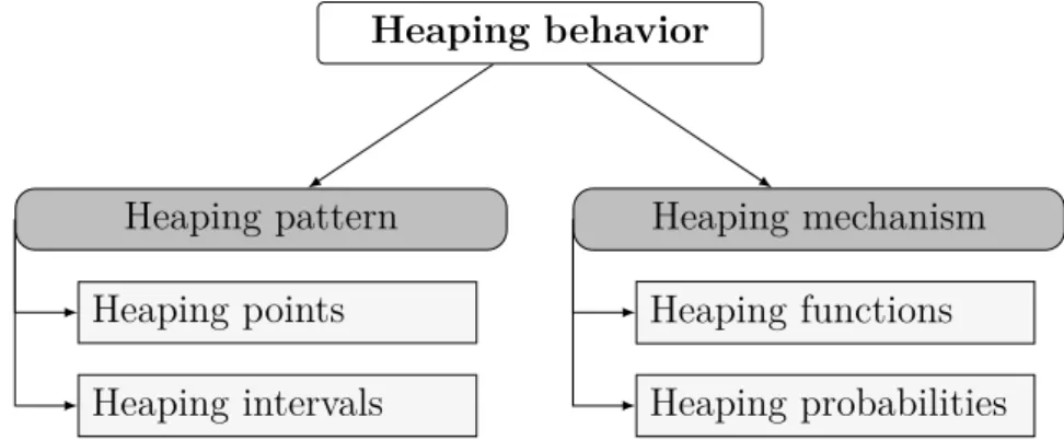
Figure 1.2: Systematization of central terms for the description of heaping.
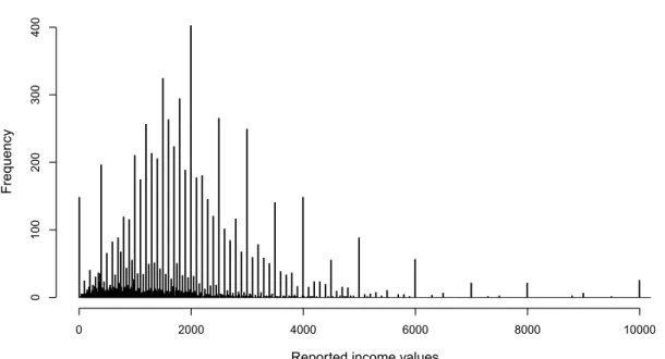
Figure 1.5: Self-reported net individual income data from the Adult Cohort in the NEPS wave 2009/2010, n = 8685 ( ≤ 10,000 EUR).
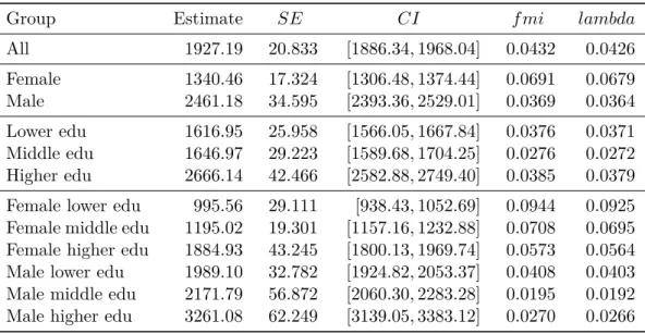
Table 1.5: Combined mean statistics for net income, divided by subgroups.
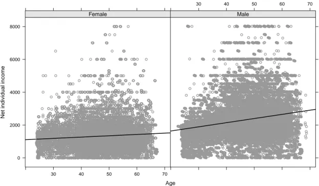
Figure 1.6: Net individual income of females and males by age.
+7

Referenzen

ÄHNLICHE DOKUMENTE

The algorithm computes an approximation of the Gaussian cumulative distribution function as defined in Equation (1). The values were calculated with the code taken

All the branch office has to do is mount a disk volume which has a copy of Datapoint's Disk Operating system and DATAPOLL on it and you can down line load

Three leading explanations are put forth for these cross-country differences: (1) other advanced economies devote a larger share of national output to transfers, which tends

4.1 LIS-Database - General characteristics and selected countries 8 4.2 Freelancers and self-employed: LIS data definitions 9 5 Income Distribution and Re-distribution in

based on the 1994 household survey. These tables yield the following importnt observations: 1) the share of wages and salaries in total income for the highest quintile was

Wage Policy in the Public Sector and Income Distribution.

For a constant price depreciation rate, both versions of the model would predict monotone relationships between mean household income and vehicle ownership statistics: a positive

For a constant price depreciation rate, both versions of the model would predict monotone relationships between mean household income and vehicle ownership statistics: a positive