Closed-Shell Hartree-Fock:
an Efficient Implementation Based on the Contraction of Integrals
in the Primitive Basis
Inaugural-Dissertation
zur
Erlangung des Doktorgrades
der Mathematisch-Naturwissenschaftlichen Fakultät der Universität zu Köln
vorgelegt von
Joseph Held aus München
Köln 2017
Tag der letzten mündlichen Prüfung: 05. Juli 2017
Meinen Eltern
Abstract
In this work a highly efficient, closed-shell restricted Hartree-Fock self-consistent-field (SCF) program has been developed. It has been written as a part of the “Quantum Objects Library” (QOL), which is developed at the Institute for Theoretical Chemistry at the University of Cologne.
In the implementation presented here, the explicit transformation of the two-electron integrals from the primitive to the radial contracted, angularly transformed basis is avoided. The density matrix is obtained by diagonalizing the Fock matrix in the radial- angular-transformed basis. It is transformed to the primitive basis, and contracted with the integrals to give the Fock matrix, also in the primitive basis. To assure that solutions of the Fock equations are obtained in the transformed basis, the Fock matrix is transformed back to the radial contracted, angularly transformed basis after the density contraction step.
Both one- and two-electron integrals are calculated using the ansatz of Obara-Saika (OS). For the evaluation of the two-electron integrals a code-generating ansatz is used.
At compile time optimized code is generated, to be called at runtime. Numerical insta- bilities inherent in the Obara-Saika scheme were analyzed and eliminated. The code- generating ansatz was also used for the implementation of the density contraction. Con- traction codes for both primitive and radial-angular-transformed bases were developed.
Both two-electron integral evaluation and density contraction implementations have been optimized by explicit use of streaming single instruction multiple data (SIMD) extensions (SSE).
Integral prescreening has been implemented on basis of the Schwarz inequality, and the differential density scheme is used. Convergence acceleration has been realized by im- plementing the direct inversion of the iterative subspace (DIIS) method. The developed SCF program has been parallelized using the open multi-processing (OMP) application programming interface (API).
In final performance comparisons to commercially available programs competitive re- sults were obtained.
In dieser Arbeit wurde ein hocheffizientes, closed-shell restricted Hartree-Fock self-consis- tent-field (SCF) Programm entwickelt. Es wurde in die "‘Quantum Objects Library"’
(QOL) integriert, die am Institut für Theoretische Chemie der Universität zu Köln ent- wickelt wird.
In der hier vorgestellten Implementierung wird die explizite Transformation der Zwei- Elektronen Integrale aus der primitiven in die radial kontrahierte, sphärisch trans- formierte Basis umgangen. Durch Diagonalisierung der Fock Matrix in der radial- sphärisch transformierten Basis wird die Dichte Matrix erhalten. Diese wird in die primitive Basis transformiert und mit den Integralen kontrahiert, wodurch die Fock Matrix ebenfalls in ihrer primitiven Darstellung vorliegt. Um sicherzustellen dass die Lösungen der Fock Gleichungen in der transformierten Basis erhalten werden, wird die Fock Matrix nach der Dichte Kontraktion zurück in die radial-sphärische Basis trans- formiert.
Sowohl Ein- als auch Zwei-Elektronen Integrale werden mit dem Verfahren von Obara- Saika (OS) berechnet, wobei für die Zwei-Elektronen Integrale ein Code generierender Ansatz gewählt wurde. Dabei wird zum Zeitpunkt der Kompilierung optimierter Code generiert, der zur Laufzeit ausgeführt wird. Die numerischen Instabilitäten des Obara- Saika Verfahrens wurden analysiert und beseitigt. Auch auf die Implementierung der Kontraktion der Dichte wurde der Code generierende Ansatz angewandt, wobei Spe- zialisierungen sowohl für primitive als auch für sphärisch transformierte Basen erzeugt wurden. beide Implementierungen, Integral Berechnung und Dichte Kontraktion, wur- den optimiert durch die explizite Berücksichtigung der streaming single instruction mul- tiple data (SIMD) extensions (SSE).
Eine Abschätzung der Integral Größenordnungen wurde auf Basis der Schwarz’schen Ungleichung umgesetzt, und das differential density scheme wird benutzt. Zur Kon- vergenz Beschleunigung kommt das direct inversion of the iterative subspace (DIIS) Verfahren zum Einsatz. Das entwickelte SCF Programm wurde mittels der open multi- processing (OMP) Programmierschnittstelle (API) parallelisiert.
In finalen Vergleichen zu kommerziell erhältlichen Programmen wurden konkurrenz- fähige Resultate im Hinblick auf die Performanz erreicht.
Contents
1. Introduction 1
I. Theory 5
2. Hartree-Fock Theory 7
2.1. Electronic Solutions for Restricted Closed-Shell Systems . . . 7
2.2. The Roothaan-Hall Equations . . . 10
3. Integral Evaluation 13 3.1. Primitive Cartesian Gaussians . . . 13
3.1.1. Shells and Shell Batches . . . 15
3.2. The Obara-Saika Scheme . . . 16
3.2.1. Overlap- and Kinetic-Energy Integrals . . . 16
3.2.2. Coulomb Integrals . . . 18
4. Symmetry In Two-Electron Integrals And Batches 23 4.1. Two-Electron Integral Symmetry . . . 23
4.2. Symmetry in Batches of Two-Electron Integrals . . . 24
5. Density Contraction 27 5.1. Integral Contributions . . . 27
5.1.1. Symmetric Integrals . . . 27
5.1.2. Integrals with Broken Symmetries . . . 28
5.2. Shell Batch Contributions . . . 29
5.2.1. Symmetric Batches . . . 29
5.2.2. Batches with Broken Symmetries . . . 29
6. Basis Transformations 31 6.1. Atomic Basis Functions . . . 31
6.1.1. The Angular Basis . . . 31
6.1.2. The Radial Basis . . . 33
6.1.3. Atomic Basis Functions in Terms of Primitive Cartesian Gaussians 33 6.2. Explicit Expressions for Basis Transformations . . . 34
6.2.1. Two-Electron Integrals . . . 34
6.2.2. The Density Matrix . . . 36
6.2.3. The Two-Electron Part of the Fock Matrix . . . 37
7. Prescreening 39
7.1. The Schwarz Inequality . . . 39
7.1.1. Batches of Integrals . . . 39
7.2. Density Screening . . . 41
7.2.1. Batches of Integrals . . . 41
7.3. The Differential Density Scheme . . . 42
II. Implementation 43
8. Technical Details 45 8.1. Programs Used . . . 458.2. Basis Sets and Geometries . . . 45
8.2.1. Basis Sets . . . 45
8.2.2. Input Geometries . . . 46
8.3. Computational Details . . . 47
8.3.1. Computational Facilities . . . 47
8.3.2. Calculational Details . . . 47
9. Numerics 49 9.1. Numerical Errors . . . 49
9.1.1. Absolute and Relative Errors . . . 50
9.1.2. Numerical Analysis . . . 50
10.Basis Sets and Iteration 55 10.1. Molecules and Basis Sets . . . 55
10.1.1. Input Format . . . 55
10.1.2. Technical Representation . . . 56
10.2. Iterators . . . 56
10.2.1. Basis Iterators . . . 57
10.2.2. Two- and Four-Index Iterators . . . 58
10.2.3. Arbitrary Level and Notation Iteration . . . 60
11.Prescreening 63 11.1. General Implementation . . . 63
11.1.1. The MapperWithMatrixAnsatz . . . 64
11.1.2. Initialization . . . 65
11.1.3. Calculation of the Estimate . . . 67
11.1.4. Accuracy . . . 68
11.1.5. Quality of the Estimate . . . 68
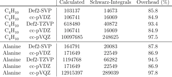
11.2. Exploiting Basis Set Hierarchies . . . 71
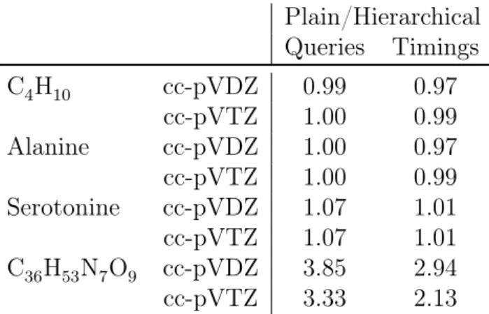
11.2.1. Results . . . 74
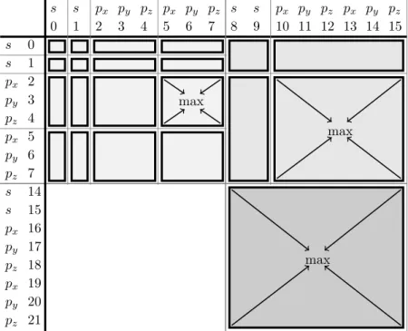
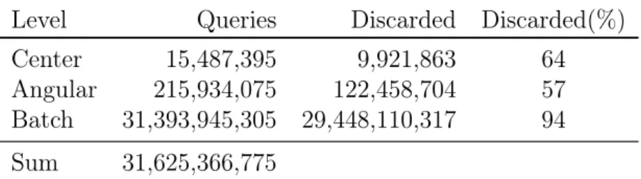
11.3. Iteration in Chemists Notation. Further Levels of Hierarchy . . . 76
11.4. The Differential Density Scheme . . . 78
Contents
12.The Obara-Saika Integration Scheme 81
12.1. General Considerations . . . 82
12.1.1. Batchwise Evaluation . . . 82
12.1.2. Batchwise Recursion . . . 83
12.1.3. Transfer Order . . . 85
12.2. Existing Implementations . . . 86
12.2.1. Generic Implementation . . . 86
12.2.2. The Code-Generation Approach . . . 87
12.3. Numerical Instabilities . . . 90
12.3.1. Solutions . . . 93
12.3.2. Results . . . 94
12.4. Code Reduction by Using a Different Code-Generating Ansatz . . . 98
12.4.1. Removing Redundancies, the Splitted Integration Ansatz . . . 99
12.4.2. Shell Ordering and Index Relations . . . 101
12.4.3. Generation of the Individual Batch Codes . . . 103
12.4.4. Comparison of the Electron Transfers E1 and E2 . . . 109
12.5. One-Electron Integrals . . . 110
13.Density Contraction 113 13.1. Existing Implementation . . . 113
13.2. Code-Generated Implementation . . . 114
13.2.1. Plain Approach . . . 114
13.2.2. Rolling the Code . . . 117
14.Fock Matrix Generation 125 14.1. Results . . . 126
14.1.1. Comparison of the Integration Codes . . . 126
14.1.2. Comparison of the Iteration Hierarchies . . . 127
14.1.3. Streaming SIMD Extensions . . . 127
III. Results 131
15.Comparisons to the TURBOMOLE and MOLPRO Program Packages 133 15.1. MOLPRO . . . 13315.1.1. Accuracy . . . 134
15.1.2. Performance . . . 138
15.2. TURBOMOLE . . . 140
15.2.1. Accuracy . . . 140
15.2.2. Performance . . . 143
16.Applications 147
IV. Summary and Outlook 151
Bibliography 155
Abbreviations and Acronyms 159
Danksagung 161
Erklärung 163
Curriculum Vitae 164
1. Introduction
The main objective of quantum chemistry is the mathematical description of atomic and molecular systems. Such systems are characterized by the Schrödinger equation [1], the required information can be obtained from the associated wave function. As closed solutions of this equation only exist for the most simple problems, approximations have to be introduced for the treatment of more complicated systems. One of the most central approximations is the restriction of the wave function to the electronic problem [2]. Two other widely used approximations are the treatment in the non-relativistic framework, and the neglection of time dependence. These three approximations are used in this work.
Even in this approximation however, except for one-electron systems, closed solutions are not available. A first, and central, ansatz to find approximate solutions for the many- electron problem has been given by Hartree and Fock [3–7]. In Hartree-Fock theory, the many-electron problem is transformed to effective one-electron problems, in which the influence of the remaining electrons is treated in an average way. However, the obtained integro-differential equations are still complicated to solve. Only further approximations made these equations applicable to a wider range of problems. By projection to a finite space, i.e. by introducing finite basis sets, the complicated integro-differential equations can be formulated as rather simple matrix problems. In the restricted (spin-free), closed- shell formulation, which this work is concerned about, the matrix eigenvalue equation of Roothaan and Hall [8, 9] is obtained. As the Fock matrix to be diagonalized in this equation depends on its solution, the Roothaan-Hall equation has to be solved iteratively.
Starting with an guess for the solutions, these equations are solved iteratively, until the corresponding field becomes self-consistent.
Even neglecting electron correlation, the ground state wave function obtained from the Hartree-Fock equations is not sufficient to describe all systems accurately. Nevertheless, Hartree-Fock theory still plays a central role in quantum chemistry. Despite the age of the theory, the wave functions obtained from Hartree-Fock calculations are widely used.
They constitute the entry point for a multitude of advanced ab-initio calculations.
With increasing computational resources and advances in theory, programs were made available to treat a variety of chemical problems in an standardized way. Still, vast resources are needed to address even systems of moderate size. Over the years, a lot of development [10–12] has been invested in optimizing the algorithms involved in the calculation of the Hartree-Fock ground state wave function. Target of most of these optimizations is the efficient treatment of the vast number of two-electron integrals arising. They scale with the fourth power of the system size and constitute a bottleneck of Hartree-Fock calculations. Various compromises have therefore been introduced, to computationally simplify the evaluation of those integrals.
Among the first of these compromises has been the development of direct SCF calcula- tions [13]. Theoretically, the two-electron integrals stay constant in each SCF iteration.
In the first implementations, they were therefore calculated once, and stored to disk. In these conventional SCF calculations however, the treatable system size is limited by the physically available disk space. In direct implementations, the integrals are recalculated in each iteration, and processed immediately. By removing the disk size limitations, larger systems became accessible, although at the cost of increased computational time.
In the long run, the direct implementation became state of the art. This is also due to the advent of advanced prescreening [14, 15] methods, by which a large number of integrals can be neglected. Especially in the context of the differential density scheme [13, 14, 16], the calculation of a certain integral can be dynamically determined in each iteration.
One of the major breakthroughs however has been the introduction of primitive Carte- sian Gaussians [17] as basis functions. Using these functions constitutes another com- promise of theory and technical realization. Although rather poorly suited to describe the physical reality, they are now used almost exclusively in electronic structure calcu- lations. This is due to the fact that they greatly simplify the calculation of the costly two-electron integrals. Their lack of physical description is accounted for by increasing the number of functions included, thus spanning the space required for a certain accu- racy. In practice, the correct radial description is achieved by linear combinations of several primitive Cartesian Gaussians of differing exponents. Another set of linear com- binations transforms these functions to spherical harmonics. This has implications to the practical realization, as quantities have to be transformed from and to this different basis sets. Nevertheless the ease of integration of primitive Cartesian Gaussians justifies these implications.
The restricted, closed-shell SCF implementation presented in this work now focuses on these implications. In common implementations, the transformation to the radial contracted and angularly-transformed basis is applied to the primitive integrals. These transformed integrals are then contracted with the transformed density. In this work a different ansatz is implemented. The contraction of the density with the integrals is performed in the primitive basis. After diagonalizing the Fock matrix, in the transformed basis, the resulting density is transformed to the primitive basis. After contraction with the primitive integrals the resulting Fock matrix is then transformed back to the radial- angular basis. Thus it is assured that the actual solution of the Fock equations is obtained in the transformed basis.
The restricted, closed-shell SCF program presented here has been written as part of the Quantum Objects Library (QOL) [18] program package of the Institute for Theoreti- cal Chemistry at the University of Cologne. Most of the techniques used in commercially available programs were included. Thus the results presented here constitute not a proof of concept study, but a fully comparable production code. Among the techniques imple- mented are integral prescreening based on the Schwarz inequality, in the context of the differential density scheme. Convergence acceleration is used with the direct inversion of the iterative subspace (DIIS) [19] ansatz. One- and two-electron integrals are calculated using the Obara-Saika scheme [20, 21]. For the two-electron integrals a highly efficient code-generated ansatz has been chosen, in which the integration code is automatically
generated at compile time, for arbitrary integrals. The density contraction also has been implemented using the code-generating ansatz. At compile time, efficient code is generated to be called at runtime. This has been done for contractions in primitive bases, as well as for contractions in spherical-harmonic basis sets. Both integration and contraction have been optimized by explicit use of streaming single instruction multiple data (SIMD) extensions (SSE).
Part I.
Theory
2. Hartree-Fock Theory
In this chapter, the key steps of the derivation of the restricted closed-shell Hartree- Fock equations will be shown. The discussion given here follows the books of Szabo and Ostlund [22], Levine [23] and Helgaker, Jørgensen and Olsen [24], to which the reader is referred to for more detailed informations.
2.1. Electronic Solutions for Restricted Closed-Shell Systems
Quantum chemistry is concerned with finding approximate solutions for the non-rela- tivistic, time independent Schrödinger equation.
HΨ =ˆ EΨ (2.1)
The Hamilton operator Hˆ =−
N
X
i=1
1 2∇2i −
M
X
A=1
1
2MA∇2A−
N
X
i=1 M
X
A=1
ZA riA +
N
X
i=1 N
X
j>i
1 rij +
M
X
A=1 M
X
B>A
ZAZB
rAB (2.2) describes the interactions of the M nuclei and N electrons of the system of interest, using the indices A and B to indicate nuclei, and i and j for the electrons. The first two terms describe the kinetic energies of electrons and nuclei. The third their Coulomb attraction. The fourth and fifth the repulsion of electrons and nuclei, respectively. MAis the mass ratio of nucleus Ato an electron,ZA the charge of that nucleus. The distances of nuclei and electrons are depicted by r.
In the Born-Oppenheimer [2] approximation the fact is used that electrons move much faster than nuclei. They can be considered to move in the field of fixed nuclei. Within this approximation, the second term of (2.2), the kinetic energy of the nuclei, can be neglected and the nuclear repulsion is just a constant. In this ansatz, the electronic problem is solved using the electronic hamiltonian.
Hˆelec =−
N
X
i=1
1 2∇2i −
N
X
i=1 M
X
A=1
ZA riA +
N
X
i=1 N
X
j>i
1
rij (2.3)
Finding approximate solutions for the electronic Schrödinger equation is the concern of Hartree-Fock theory.
HˆelecΦelec =EelecΦelec (2.4)
The solutions of this equation depend parametrically on the coordinates of the nuclei, giving different wave functions and energies for different nuclear arrangements.
To obtain the total energy of the system, the constant nuclear repulsion has to be taken into account.
Etot =Eelec+
M
X
A=1 M
X
B>A
ZAZB
rAB (2.5)
As this work is only concerned with solutions of the electronic Schrödinger equation (2.4), the subscriptelec to the hamiltonian, energy and wave function will be dropped in the following.
The electronic wave function will be set up from linear combinations of products of spin orbitals. In a spin orbital χ, one electron is described by the product of its spatial distributionψ(r)and one of the two spin functions α(ω)or β(ω).
χ(x) = ψ(r)α(ω) or χ(x) =ψ(r)β(ω) (2.6) Here the spatial and spin coordinates r and ω are collected to x. The spatial orbitals are assumed to form an orthonormal set, from which orthonormality in the set of the spin orbitals follows.
Z
χ∗i(r)χj(r)dr =hχi|χji=δij (2.7) To account for the indistinguishability of the electrons and the antisymmetry of the wave function, Slater determinants [25] are used to set up the wave function.
Φ(x1, x2, . . . , xN) = (N!)−1/2
χi(x1) χj(x1) · · · χk(x1) χi(x2) χj(x2) · · · χk(x2)
... ... ...
χi(xN) χj(xN) · · · χk(xN)
≡ |χiχj. . . χki (2.8)
In this Slater determinant,N electrons occupyN spin orbitals. No specification is made as to which electron occupies which spin orbital, thus ensuring indistinguishability. An- tisymmetry is met by the mathematical properties of the determinant [26]. Interchange of two rows changes the sign of the determinant. This corresponds to an interchange of two electrons. The Pauli exclusion principle [27] is met by another property of the de- terminant. Two electrons occupying the same spin orbital results in two equal columns, for which the determinant is zero.
In Hartree-Fock theory, a single determinant ansatz is used to describe the ground state of anN-electron system.
|Φ0i=|χ1χ2. . . χNi (2.9) Specifically, this work is concerned with solutions for closed-shell systems, using a set
2.1. Electronic Solutions for Restricted Closed-Shell Systems of restricted spin orbitals. In a restricted set of spin orbitals, two spin orbitals χ(x) are built from one spatial orbital ψ(r), one withα- and the other withβ-spin, respectively.
In a closed-shell system withN electrons, the ground state is then built fromN/2spatial orbitals, each of which is doubly occupied.
|Φ0i=|ψ1α ψ1β · · · ψN/2α ψN/2βi (2.10) The expectation value for the ground state energy can be expressed in terms of spatial orbitals. Application of the Slater-Condon [28, 29] rules and integrating out spin gives the Hartree-Fock ground state energy E0.
E0 =hΦ0|H|Φˆ 0i=
N/2
X
i
hi|ˆh|ii+1 2
N/2
X
ij
(2hij|iji − hii|jji) (2.11) Here, the one-electron part of the hamiltonian is given by
hi|ˆh|ji= Z
ψi∗(r1) −1 2∇2−
M
X
A
ZA r1A
!
ψj(r1)dr1 (2.12) and the two-electron part by
hij|kli= Z Z
ψi∗(r1)ψj∗(r2) 1
r12ψk(r1)ψl(r2)dr1dr2 (2.13) Note that the physicists notation will be used for all two-electron integrals over spatial functions. The specific nature of those functions will be implied by the context.
Now the variational principle states that the expectation value of the trial function
|Φ0i is always greater than or equal to the exact electronic energy.
E ≤ hΦ0|H|Φˆ 0i=E0 (2.14)
The strategy is then to minimize E0 by varying the spatial orbitals ψ. This can be done using Lagranges’ method of undetermined multipliers, under the constraint of orthonormal spatial orbitals. Doing so leads to the restricted, canonical closed-shell Fock equation.
fˆ|ψai=a|ψai (2.15)
It is of the eigenvalue form, determining the spatial orbitals and their energy . The restricted, closed-shell Fock operator is defined as
fˆ(1) = ˆh(1) +
N/2
X
b
2 ˆJb(1)−Kˆb(1)
(2.16) It is an effective one-electron operator. Similar to (2.12), operators depending only on
the coordinate of one electron are collected in the one-electron operatorˆh.
ˆh(1) =−1
2∇21−X
A
ZA
r1A (2.17)
The effects of the other electrons are included in an averaged way by the summation over the two-electron operators Jˆand K. The local Coulomb operatorˆ
Jˆb(1)ψa(1) =
Z ψb∗(2)ψb(2) r12
dx2
ψa(1) (2.18)
can be interpreted as a classical potential. The non-local exchange operator Kˆb(1)ψa(1) =
Z ψ∗b(2)ψa(2) r12 dx2
ψb(1) (2.19)
has no classical interpretation.
2.2. The Roothaan-Hall Equations
The integro-differential equation (2.15) can be turned into a set of algebraic equations, which can be solved by standard matrix techniques. After Roothaan, this is accomplished by introducing a set ofk known basis functionsφ, in which the molecular orbital (MO) ψ are linearly expanded.
ψl=
k
X
j
Cjlφj (2.20)
Using this expansion in (2.15), multiplying with φ∗m on the left and integrating, the Roothaan equations are obtained.
k
X
j
Cjl Z
φ∗m(1) ˆf(1)φj(1)dr1 =l
k
X
j
Cjl Z
φ∗m(1)φj(1)dr1 (2.21) Introducing the Fock
Fmj = Z
φ∗m(1) ˆf(1)φj(1)dr1 (2.22) and the overlap matrix
Smj = Z
φ∗m(1)φj(1)dr1 (2.23)
2.2. The Roothaan-Hall Equations
the Roothaan Hall equations can be written in the generalized eigenvalue form.
FC=SC (2.24)
The Fock matrix is
F=Hcore+G (2.25)
where the one-electron partHcoreis the sum of kinetic- and nuclear attraction integrals.
Hijcore=−1 2
Z
φ∗i(1)∇2φj(1)dr1−X
A
Z
φ∗i(1)ZA
r1Aφj(1)dr1 (2.26)
=Tij +Vij (2.27)
For the two-electron part G, in terms of two-electron integrals over the basis functions
|ii=φi(r), the following is obtained.
Gij =X
kl
Dkl
hik|jli − 1
2hik|lji
(2.28) Here the density matrix Dhas been introduced as the product of the ’occupied’ columns of the expansion coefficients.
Dij = 2
N/2
X
k
CikCjk∗ ≡Cocc·C∗occ (2.29)
3. Integral Evaluation
Integrals over basis functions are of central importance in electronic structure theory, both from a theoretical and technical point of view. In technical terms, this is due to the sheer number of integrals arising already for calculations of small systems. Especially the two-electron integrals, scaling with the fourth power of the number of basis functions, turn out to be rather demanding in terms of computational resources. An optimal implementation is therefore mandatory for highly efficient production codes.
Several schemes exist to evaluate integrals over basis functions. This work focuses on the implementation of the recurrence relations of Obara and Saika [20, 21]. Other evaluation schemes, such as the Gaussian quadrature [30, 31], the McMurchie-Davidson scheme [32] and the method of Pople et al. [33, 34] will not be discussed.
It shall be noted that most of the discussion given in this chapter follows the one given in the book of Helgaker, Jørgensen and Olsen [24].
3.1. Primitive Cartesian Gaussians
Of great importance is the choice of basis functions to be integrated over. In the long run, primitive Cartesian Gaussian (PCG) [17] functions became the state of art, trading their lack of correct physical description for ease of integration [24]. They are specified by an exponent a, a center A and have a total angular momentum ofl =i+j+k,
Gi j k
(r, a, A) =xiAyAjzkAexp(−ar2A) =Ga(r). (3.1) The vectorrA=r−Ais the distance relative to the center. Note that in the abbreviated form Ga(r), exponent, center and angular momentum information are collected to the single index a.
Their main advantage is that they are separable with respect to the three Cartesian directions:
exp −a q
x2A+y2A+zA2 2!
= exp(−ax2A) exp(−ayA2) exp(−azA2) (3.2) This drastically simplifies the evaluation of integrals. The physically better suited Slater type functions lack this separability.
exp(−arA) = exp
−aq
x2A+yA2 +zA2
6=f(x)f(y)f(z) (3.3)
Another property is that the product of two (or any number of) PCG’s can be written in terms of a different, single PCG. This is the Gaussian product rule [17]. Separability can be used, giving the product of two spherical (l = 0) Gaussians in x-direction as
exp(−ax2A)·exp(−bx2B) =Kabx exp(−px2P) (3.4) Where
p=a+b (3.5)
Px = aAx+bBx
p (3.6)
XAB =Ax−B (3.7)
µ= ab
a+b (3.8)
Kabx = exp(−µXAB2 ) (3.9) For arbitrary l, the one-dimensional Gaussian overlap distribution is just
Ωxij(x) = xiAxjBKabx ·exp(−px2p) (3.10) Applying this to all Cartesian direction, the general, three-dimensional Gaussian overlap distributionΩab(r) = Ga(r)·Gb(r) can be split up into one-dimensional parts
Ωab(r) = Ωij mnkl
(r) = Ωxij(x)Ωykl(y)Ωzmn(z) (3.11) The trivial relationships
Ωxi+1,j =xAΩxij (3.12)
Ωxi,j+1 =xBΩxij (3.13)
lead to the recurrence relation
Ωxi,j+1−Ωxi+1,j =XABΩxij. (3.14)
Finally, the derivatives of the Gaussian overlap distributions with respect to the center coordinates are
∂Ωxij
∂Ax = 2aΩxi+1,j−iΩxi−1,j (3.15)
∂Ωxij
∂Bx = 2bΩxi,j+1−iΩxi,j−1 (3.16)
3.1. Primitive Cartesian Gaussians
3.1.1. Shells and Shell Batches
Central to all integration schemes presented in this work is the concept of grouping basis functions into shells. A shell is defined as the set of functions located on the same center and having the same angular momentum and exponent. For l = 1, some center A and some exponent a, this particular p-shell consists of the three functions
pAa,x =xAexp(−ar2A) (3.17) pAa,y=yAexp(−ar2A) (3.18) pAa,z =zAexp(−arA2) (3.19) Mostly, shells will be addressed solely by their angular momentum, i.e. p, f and so on.
If a distinction for shells of equal angular momenta has to be made, a combined index will be used, i.e. a pi-shell is supposed to have a different center and or exponent than a pj-shell.
Generally, the number of PCG’s in a given shell of angular momentum l is Nlpcg = (l+ 1)(l+ 2)
2 (3.20)
A shell batch is the set of integrals arising from the combination of two (one-electron integrals) or four (two-electron integrals) shells. Again, shells will be denoted by their angular momenta, using indices when necessary. The two-electrondpss-batch for exam- ple can have two distinctive (dpsisj), or equal (dpsisi) s-shells.
Consider for example the shell batchpipjsksl, with arbitrary labeled functions.
pipjsksl≡
h
a b c
d e f
|(g) (h)i
Combining the functions in the shells leads to the following nine integrals. The order of the functions is in accordance to the order of the shells. Permutations of the shells leading to an according permutation of the functions in the integrals.
had|ghi hbd|ghi hcd|ghi hae|ghi hbe|ghi hce|ghi haf|ghi hbf|ghi hcf|ghi
The generation of the integrals of a batch is just the Cartesian product of the four sets of functions (shells): {a, b, c}x{d, e, f}x{g}x{h}. In this case the Cartesian product is associative.
Neglecting redundancies, the number of integrals present in a batch is then just the product of the shell sizes.
The reason to impose this grouping of integrals into batches is technical, based on the reusage of shared quantities within the calculation of integrals of a given batch. For
example, all prefactors (3.5) to (3.9) of a Gaussian overlap distribution (3.11) depend only on the exponents (a and b) and centers (A and B). Thus, computing them once prior to the evaluation of allNl,i·Nl,j Gaussian overlap distributions, and reusing them when needed, clearly saves computational cost compared to repeated recomputation.
Additionally, the integration schemes used for this work are recursive, involving a lot of intermediates. Again, most of these intermediates are needed for the calculation of different integrals in a given batch. Calculation of one batch as a whole exploits this by reusing those intermediates, compared to a costly recalculation in an individual integral evaluation scheme.
3.2. The Obara-Saika Scheme
In this work, the recurrence relations derived by Obara et al. [20, 21] will be used to evaluate all integrals necessary for a Hartree-Fock SCF calculation. It will be used in the modified version introduced by Head-Gordon and Pople [35], Hamilton and Schäfer [36]
and Lindh, Ryu and Liu [37].
Generally, integrals over PCG’s of specific angular momenta are expressed in terms of integrals of in- or decreased angular momenta. Starting with integrals over spherical PCG’s (l = 0), integrals for higher angular momenta can be obtained by application of the recurrence relations. For the spherical recursion seeds analytical expressions are known.
Each PCG has three dimensions of angular momentum l = i+j +k. To specify a one-electron integral (two PCG’s), six indices are needed, 12 for a two-electron integral (four PCG’s), respectively. However, based on the separability of the PCG’s, there is no mixing of directions in the Obara-Saika schemes. To increment some angular momentum inx-direction, only in- or decrements in thex-direction are needed. This allows for some simplification in the notation, by omitting the unneeded directions. The actual direction the recurrence relation is applied to is given implicitly by the direction of the associated center coordinate.
Explicit derivations will be shown for the one-electron overlap and kinetic-energy integrals. For Coulomb integrals, both one- and two-electron, the derivation will be skipped, an extensive derivation can be found in the book of Helgaker et al. [24].
3.2.1. Overlap- and Kinetic-Energy Integrals
Overlap Integrals
The overlap integrals Sab are of the form Sab =
Z ∞
−∞
G∗a(r)Gb(r)dr =ha|bi (3.21) As the PCG’s used in this work are real, complex conjugation has no effect and will be omitted from now on (this concerns all integrals over PCG’s). Thus, the overlap
3.2. The Obara-Saika Scheme integrals are just integrals over a Gaussian overlap distribution and can be separated in the three Cartesian directions.
Sab = Z ∞
−∞
Ωab dr (3.22)
= Z ∞
−∞
Ωxij dx Z ∞
−∞
Ωykl dy Z ∞
−∞
Ωzmn dz
=Sijx Skly Smnz
The horizontal recurrence relation follows directly from integrating (3.14):
Si,j+1x −Si+1,jx =XABSijx (3.23)
Additionally, the overlap integrals are invariant to identical translations of the centers A and B
∂Sijx
∂Ax + ∂Sijx
∂Bx = 0 (3.24)
Insertion of the definition (3.22) and application of the derivatives of the Gaussian overlap distributions (3.15) and (3.16) then gives the recurrence relation
2aSi+1,jx −iSi−1,jx + 2bSi,j+1x −jSi,j−1x = 0 (3.25) Finally, using the horizontal recursion (3.23), the Obara-Saika recurrence relations for the overlap integrals can be obtained
Si+1,jx =XP ASijx + 1
2p iSi−1,jx +jSi,j−1x
(3.26) Si,j+1x =XP BSijx + 1
2p iSi−1,jx +jSi,j−1x
(3.27) The center of chargeP and the total exponentphave their origin in the Gaussian overlap distribution, eqns. (3.6) and (3.5), respectively.
The recursion seed, S00x is just the integral of a spherical Gaussian distribution S00x =Kabx
Z ∞
−∞
exp(−px2P) =Kabx rπ
p (3.28)
The actual overlap integral Sab can then be calculated from (3.22).
Kinetic-Energy Integrals The kinetic-energy integrals
Tab = Z ∞
−∞
Ga(r)(−1
2∇2)Gb(r)dr =ha|Tˆ|bi (3.29)
are closely related to the overlap integrals. In a first step, the integral is separated into Cartesian directions via the Laplace-operator
Tab =−1 2
hGa| ∂2
∂x2|Gbi+hGa| ∂2
∂y2|Gbi+hGa| ∂2
∂z2|Gbi
(3.30) Now the separability of the PCG’s shows the dependence on the overlap integrals
−1
2hGa| ∂2
∂x2|Gbi=SklySmnz
−1
2hGxi| ∂2
∂x2|Gxji
=SklySmnz Tijx (3.31) which gives the total kinetic-energy integral as
Tab =TijxSklxSmnx +SijyTklySmny +SijzSklzTmnz (3.32) Using
∂Gxi
∂x =−∂Gxi
∂Ax (3.33)
the kinetic-energy integral can be written in terms of a differentiated overlap integral Tijx =−1
2hGxi| ∂2
∂x2|Gxji=−1 2
∂2
∂A2xSijx (3.34)
The final recurrence relations for the one dimensional kinetic-energy integrals can then be obtained by differentiation of the overlap recurrence relations (3.26) and (3.27) with respect toAx.
Ti+1,jx =XP ATijx + 1
2p iTi−1,jx +jTi,j−1x + b
p 2aSi+1,jx −iSi−1,jx
(3.35) Ti,j+1x =XP BTijx+ 1
2p iTi−1,jx +jTi,j−1x + a
p 2bSi,j+1x −iSi,j−1x
(3.36) The recursion seed is
T00x =
a−2a2
XP A2 + 1 2p
S00x (3.37)
3.2.2. Coulomb Integrals
The derivation of the Coulomb integrals Z ∞
−∞
Ga(r)Gb(r)
rC dr =ha| 1
rC|bi (3.38)
3.2. The Obara-Saika Scheme
and
Z ∞
−∞
Z ∞
−∞
Ga(r1)Gc(r2)Gb(r1)Gd(r2) r12
dr1dr2 =hac|bdi (3.39) shall not be repeated here, only key steps will be shown. An extensive derivation can be found in the book of Helgaker et al. [24].
The Boys Function
Central to the evaluation of the Coulomb integrals (3.38) and (3.39) is the inverse dis- tance operator 1r. Due to its presence, the Coulomb integrals can not be factored in the Cartesian directions. However, the inverse distance operator can be expressed as an one-dimensional integral over a spherical PCG.
1 r = 1
√π Z ∞
−∞
exp(−r2t2)dt (3.40)
This is the key step in the evaluation of Coulomb integral over PCG’s. It leads to their expression in terms of a special class of functions, the Boys function [17]
FN(x) = Z 1
0
exp(−xt2)t2Ndt (3.41) The integration over the whole one- or two-particle space has been reduced to a one- dimensional integration over a fixed interval.
One-Electron Integrals
The Obara-Saika recurrence relations for the one-electron Coulomb integrals are ex- pressed in terms of auxiliary integrals ΘNij;kl;mn. The superscript N having its origin in the order of the Boys function and the subscripts specifying the angular momenta inx-, y- andz-direction. The integrals with N = 0 are the actual Coulomb integrals.
Θ0ij
mnkl
=ha| 1 rC
|bi (3.42)
Similar to the overlap and kinetic-energy integrals, recurrence relations exist to increase angular momenta for the bra-index i.
ΘNi+1,j =XP AΘNij + 1
2p iΘNi−1,j+jΘNi,j−1
−XP CΘNij+1− 1
2p iΘN+1i−1,j+jΘN+1i,j−1
(3.43) Again, the prefactors arising from the Gaussian overlap distribution (3.5) to (3.9). For the ket-index j the horizontal recurrence relation
ΘNi,j+1 = ΘNi+1,j+XABΘNij (3.44)
is obtained.
Note that the recurrence relations operate solely within some Cartesian direction (here:
x-direction), thus indices for the remaining (untouched) directions have been omitted.
The direction of the recurrence is implicitly stated by the prefactors (XIJ). Additionally, and contrary to the kinetic-energy and overlap integrals, the Coulomb integrals depend on the parameter N. It is introduced by the recursion seeds, which are given by the scaled Boys function of order N.
ΘN00
0000
= 2π
p KabxyzFN(pR2P C) (3.45) Here, the one dimensional pre-exponential factors have been abbreviated to (see eqn.
(3.9)).
Kabxyz =KabxKaby Kabz (3.46)
Two-Electron Integrals
Similarly to the one-electron Coulomb integrals, the two-electron integrals are expressed in terms of the auxiliary integrals ΘNijkl;mnop;qrst. Again, N is connected to the Boys function and the subscripts specify the angular momenta of the integral. The zeroth order in N integrals are the two-electron Coulomb integrals
Θ0ijkl
mnop qrst
=hac|bdi (3.47)
The recursion seeds are given by the scaled Boys function of order N. ΘN0000
00000000
= 2π5/2 pq√
p+qKabxyzKcdxyzFN(αR2P Q) (3.48) In principle, recursion relations for each index can be obtained from the original Obara- Saika recurrence relation
ΘNi+1,jkl =XP AΘNijkl−α
pXP QΘN+1ijkl + i 2p
ΘNi−1,jkl−α
pΘN+1i−1,jkl
+ j
2(p+q)ΘN+1i,j−1,kl+ k 2p
ΘNij,k−1,l− α
2pΘN+1ij,k−1,l
+ l
2(p+q)ΘNijk,l−1+1 (3.49) Here, q and Q are the equivalents of p and P, related to Gc and Gd. The reduced exponentα is
α= pq
p+q (3.50)
3.2. The Obara-Saika Scheme Using index substitution and renaming variables leads to the recurrence relation for the j index.
ΘNi,j+1,kl =XQCΘNijkl+α
qXP QΘNijkl+1+ j 2q
ΘNi,j−1,kl− α
qΘNi,j−1,kl+1
+ i
2(p+q)ΘN+1i−1,jkl+ l 2q
ΘNijk,l−1− α
qΘNijk,l−1+1
+ k
2(p+q)ΘNij,k−1,l+1 (3.51) Similar equations can be found for thekandlindices, respectively. Using these equations leads to rather complicated expressions, as each recurrence involves up to eight contri- butions and recurrences in every index. Fortunately, a four step ansatz exists [35–37], using simpler recurrence relations.
By setting j = k =l = 0 in (3.49), the vertical recurrence relation for the i-index is obtained.
ΘNi+1,000 =XP AΘNi,000− α
pXP QΘN+1i,000+ i 2p
ΘNi−1,000− α
pΘNi−1,000+1
(3.52) Using translational invariance (compare (3.24)), increments in the j-index can be gen- erated using the electron transfer recursion.
ΘNi,j+1,00=−bXAB+dXCD
q ΘNi,j,00+ i
2qΘNi−1,j,00+ j
2qΘNi,j−1,00−p
qΘNi+1,j,00 (3.53) Similarly to (3.52), a different electron transfer can be obtained by setting l =k = 0 in (3.51).
ΘNi,j+1,00 =XQCΘNij00+α
qXP QΘNij00+1+ i
2(p+q)ΘN+1i−1,j00 +j
2q
ΘNi,j−1,00−α
qΘNi,j−1,00+1
(3.54) Finally, increments for the k- and l-index are generated by the horizontal recursions (compare (3.14)).
ΘNi,j,k+1,l = ΘNi+1,j,k,l +XABΘNi,j,k,l (3.55) ΘNi,j,k,l+1 = ΘNi,j+1,k,l+XCDΘNi,j,k,l (3.56)
4. Symmetry In Two-Electron Integrals And Batches
Generally put, the bottleneck of the assembly of the Fock matrix is the number of two- electron integrals to be calculated and contracted with the density matrix. They scale with the fourth power of the basis functions present in the system of interest. One way to reduce the number of integrals to be calculated is to take symmetries into account.
This reduces the number of significant integrals by about an factor of eight.
4.1. Two-Electron Integral Symmetry
The general integral over PCG’s is of the form hpr|qsi=
Z
Gp(r1)Gr(r2) 1
r12Gq(r1)Gs(r2)dr12 (4.1) There are three symmetries leaving this integral invariant. Clearly, the interchange of the basis functions depending on r1, Gp(r1) and Gq(r1), does not change the value of the integral.
hpr|qsi=hqr|psi (4.2)
This holds equivalently for the functions depending on r2.
hpr|qsi=hps|qri (4.3)
Finally, the two-electron integrals are invariant with respect to particle exchange, giving
hpr|qsi=hrq|sqi (4.4)
Each of these symmetries only leads to equivalent integrals if certain inequalities con- cerning the involved functions are met. For the particle one symmetry, interchange of the bra1 and ket1 functions only leads to a symmetry equivalent integral if
p6=q (4.5)
In integrals where p = q, particle one exchange just produces the same integral again, hpr|psi → hpr|psi. Obviously, this also holds for the other two symmetries as well.
Particle two symmetry, or exchange of the bra2 with the ket2 function, only gives a
symmetry-equivalent integral if
r6=s (4.6)
Finally particle exchange symmetry is met if
p6=r and q 6=s (4.7)
Each of these symmetries, if present, doubles the number of symmetry equivalent inte- grals. The total number nse of symmetry equivalent integrals for an index combination with s symmetries present is just
nse = 2s (4.8)
In the integral hpp|ppi, no symmetry is present and nse = 1. No symmetry equivalent integrals exist. On the other hand, in the integral hpr|qsi, all three symmetries are present, nse = 8 and seven symmetry equivalent integrals can be found. An example for an integral with one symmetry present is hpr|pri. Particle exchange gives the one symmetry equivalent integral as hrp|rpi.
Integral ’classes’ with all three symmetries present will be termed as symmetric. Asym- metric classes are then the ones having one or more symmetries broken, respectively.
The idea now is to exploit this during the integral evaluation. Instead of calculating allnsesymmetry-equivalent integrals, only one ’non-redundant’ integral of the particular class is calculated. The exact number of non-redundant two-electron integrals in a system with n basis functions is
Nnr = 1
8(n4+ 2n3+ 3n2+ 2n) (4.9) Taking this into account, of all the n4 integrals, only about one eighth have to be calculated.
4.2. Symmetry in Batches of Two-Electron Integrals
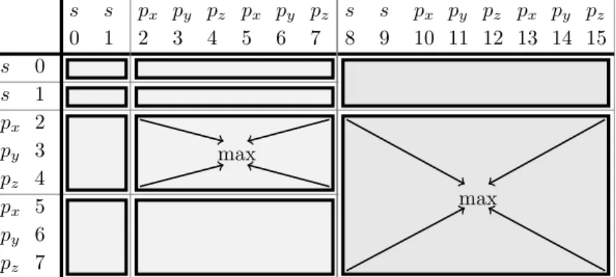
As explained in section 3.1.1, then basis functions are grouped into shells. The integrals arising from some tuple of shells are called shell batches. Now the symmetry properties of the two-electron integrals can equally be applied to four-tuple shell batches. Introducing a p-shell to be holding the three p-functionspx, py and pz, and an s-shell to be holding one s-function, some psss-batch will consist of the integrals
pisjsksl ≡
pi,x
pi,y pi,z
sjsksl
≡
hpi,xsj|sksli hpi,ysj|sksli hpi,zsj|sksli
4.2. Symmetry in Batches of Two-Electron Integrals Particle exchange gives the three integrals hsjpi,x|slski, hsjpi,y|slski and hsjpi,z|slski, which are contained in the shell batch sjpxslsk.
This is generally applicable, the rules being identical to those for the two-electron inte- grals, replacing functions with shells. The total number of non-redundant shell batches is also given by equation (4.9), substituting the number of basis functions n with the number of shells. The set of non-redundant shell batches holds all non-redundant inte- grals. However, some redundant integrals are reintroduced if the tuple is asymmetric.
In the pipisisi batch for example the particle exchange symmetry (4.7) is broken. The batch contains, among others, the integrals hpi,xpi,y|sisii and hpi,ypi,x|sisii which are symmetrically identical. There is no simple formula to calculate the number of redun- dancies reintroduced this way. Table 4.1 shows the percentage of redundant integrals introduced in the set of non-redundant batches for some model systems. Their number clearly decreases with increasing molecule and/or basis size to a negligible amount. Even for high percentages however, the technical benefits from calculating integrals as batches outweigh the overhead introduced (see section 12.1.1).
cc-pVDZ cc-pVTZ cc-pVQZ cc-pV5Z cc-pV6Z
CH4 5.19 5.24 4.42 3.46 2.76
C2H6 3.13 3.18 2.70 2.12 1.70
C4H10 1.74 1.78 1.52 1.20 0.96
C6H14 1.21 1.23 1.05 0.83 0.67
C8H18 0.92 0.94 0.81 0.64 0.51
Table 4.1.: Percentage of redundant integrals in the set of non-redundant batches Concluding, the exploitation of integral symmetries by omitting the calculation of re- dundant integrals can be done in terms of non-redundant shell batches, the overhead reintroduced being negligible.
5. Density Contraction
In Hartree-Fock theory, the two-electron part G of the Fock matrix is calculated by contraction of the density matrix D with the two-electron integralshij|kli
Gij =X
kl
Dkl[hik|jli −0.5hik|lji] (5.1) This step is of the order of integrals, making an efficient implementation mandatory. As the integration is performed on the basis of integral batches, the approaches to density contraction presented in this work are also in terms of a batchwise contraction.
5.1. Integral Contributions
Central aspect of the ansatz presented here is the exploitation of symmetry equivalent integrals. As has been shown before in section 4.1, considering only non-redundant integrals reduces the number of integrals to be taken into account by about an factor of eight. Obviously, reducing the number of integrals also reduces the amount of effort to be put into contracting them with the density, given an effective strategy can be found to be applied to eqn. (5.1). Starting point in discussing the density contraction is the analysis of the contributions of symmetry-equivalent integrals to the Fock matrix. In doing so, symmetric integrals have to be distinguished from asymmetric ones.
5.1.1. Symmetric Integrals
For each integral with four different basis functions hpr|qsi, eight symmetry equivalent ones exist. This corresponds to 16 contributions of the same integral to G. Of these, eight arise from the first integral of equation (5.1), the other eight from the second, respectively.
Gpq += Drshpr|qsi Gps −= 0.5Drqhpr|qsi Gpq += Dsrhps|qri Gpr −= 0.5Dsqhps|qri Gqp += Drshqr|psi Gqs −= 0.5Drphqr|psi Gqp += Dsrhqs|pri Gqr −= 0.5Dsphqs|pri Grs+= Dpqhrp|sqi Grq −= 0.5Dpshrp|sqi Grs+= Dqphrq|spi Grp −= 0.5Dqshrq|spi Gsr+= Dpqhsp|rqi Gsq −= 0.5Dprhsp|rqi Gsr+= Dqphsq|rpi Gsp −= 0.5Dqrhsq|rpi