TRANSIT
Ultrafast Shortest-Path Queries with Linear-Time Preprocessing
Andreas Heider October 15, 2010
Abstract
First some general techniques how to speed up shortest path queries are introduced and then TRANSIT, an algorithm that makes use of these techniques to answer shortest distance queries in almost linear time. Later this is extended to shortest path queries and further improvements are described.
Contents
1 Introduction 3
1.1 Overview . . . 3
1.2 Basic Techniques . . . 3
2 Transit Node Routing 3 2.1 The key observation . . . 3
2.2 Algorithm outline . . . 4
2.3 How to implement ‘far’ . . . 4
2.4 The preprocessing step . . . 5
2.5 Computing the distance tables . . . 6
2.6 Shortest distance queries . . . 7
2.7 Shortest path queries . . . 7
2.8 Local queries . . . 7
2.9 Multi-Level Grid . . . 7
3 Conclusions 8
1 Introduction
1.1 Overview
Computing a shortest path between two points on a graph is a theoretical problem with many practical applications. One of them is finding a route on a road network, as used on many navigation devices or services like google maps.
The data set for such a road network can get very large, for example the US road network consists of about 24 million nodes or 58 million edges. Combined with the limited processing power of handheld devices and the huge amount of queries on online services this leads to the need of fast and efficient algorithms.
The classical algorithm to find shortest paths in a graph is Dijkstra’s algorithm. Although there have been numerous improvements to it, it’s complexity is still not good enough.
As a ballpark figure running Dijkstra’s algorithm to find a shortest path between two random points on a large road network and on a state of the art computer takes time in the order of a few seconds, the best algorithms of the time when the algorithm was first presented took a few milliseconds and TRANSIT queries will run in microseconds.
1.2 Basic Techniques
TRANSIT uses two main techniques to achieve this kind of performance. The first is to split the work into two parts: A preprocessing step runs beforehand and stores additional information that can be used later to speed up the queries. To do this split efficiently the ratio between additional data stored and work that has to be done in the query has to get optimized. To some extent the preprocessing time is also a factor, but as the preprocessing only needs to get done once it’s less important than the space requirement and query time.
As an example consider an algorithm that does uses a APSP algorithm as the preprocessing step and stores the shortest path to every other node in each node. This leads to perfect query times as there is nothing left to be done in to answer a query other than to lookup the result but obviously the space and preprocessing requirements are much too large for this algorithm to be used in any practical application.
The other extreme, simply not doing anything in the preprocessing step is equally useless.
So to get the most of this technique the work split has to be balanced such that as little as possible additional space usage leads to as much of a query time improvement as possible.
Secondly the algorithm doesn’t have to work on general graphs but on road networks.
Road networks exhibit some special properties that can be used to build a faster algorithm.
For example, they are almost planar, the nodes have small degree and there is some hierarchy of more and more important roads.
2 Transit Node Routing
2.1 The key observation
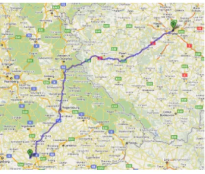
What TRANSIT bases on is a similar property. Suppose you want to travel to somewhere very far from where you live. To get there you would have to leave your neighborhood to get on probably bigger roads which lead you to your destination. The key observation is that there are only very few roads through which you will leave your neighborhood. Select nodes on these roads will be key nodes for our algorithm and will be called Transit Nodes.
Figures 1 and 2 illustrate this observation. They show two different trips, both starting at the same location but ending at different destinations. When looking at the complete paths in Figure 1 they look not at all similar, but when taking a closer look at the start of both trips
Figure 1: Two different shortest paths starting at the same location
Figure 2: The beginnings of the two shortest paths
in Figure 2 it’s easy to see that both start the same way. The red spot marks one possible Transit Node, a motorway access.
The same node is also a Transit Node for other starting points in the same neighborhood, as the shortest path for very close starting points will be largely the same.
So for each neighborhood the precomputation step has to calculate a set of Transit Nodes such that every sufficiently far shortest path starting or ending in a neighborhood will pass through one of the neighborhoods Transit Nodes.
2.2 Algorithm outline
The basic idea of TRANSIT is that every ‘far’ trip can be split in three parts: From the start point src to a transit node t1 associated with it, from that transit node to a transit node t2 associated with the destination trg. To answer a shortest distance query dist(src, trg) all that has to be done is finding the two target nodes out of all possible target nodes of the neighborhoods of srcand trg that lie on the shortest path.
dist(src, trg) =min(dist(src, t1) +dist(t1, t2) +dist(t2, trg)) (1) This can be done very fast because it’s possible to precompute all these distances. While computing the Transit Nodes in the preprocessing step, its easy to also calculate all distances dist(node, t1) from each node to all of its Transit Nodes. To get the distances dist(t1, t2) an additional APSP step for all Transit Nodes is needed.
2.3 How to implement ‘far’
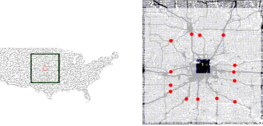
Since this approach only works for ‘far’ enough trips, some metric is needed to determine when a trip is far enough and neighborhoods need to be defined as well.
Figure 3: A neighborhood cell and its far region
One possibility to do this is to subdivide the map into a grid of cells. Each cell then is a neighborhood that all nodes inside this cell belong to. This subdivision can also be used to determine if a trip is far enough by looking at the distance between the cells the start and destination points lie in. If its greater than a certain threshold the trip is considered far enough.
Both the grid size as well as the ‘far’ threshold affect the algorithm’s performance as they determine how many trips are ‘far’ enough and how many transit nodes have to be processed.
For the threshold experiments showed that 4 is a good default value and an elegant solution for the grid size problem will be given later in the paper.
2.4 The preprocessing step
Figure 4: A cell and its surroundings
Figure 5 shows a more structured view of a cell. In the middle is the cell C itself which represents a neighborhood. The squareSouteris the border between ‘far’ and local destinations, all nodes outside this square are ‘far’ away. The squareSinner betweenC and Souter is where we will place the Transit Nodes.
LetEC/inner/outerbe the edges that crossC,Sinner orSouterrespectively andVC/inner/outer
the nodes with the lower id of every edge in EC/inner/outer.
Then it’s easy to see that every trip starting inC that is ‘far’ enough will first pass one of the nodes inVinner and then one inVouter.
A simple way to find all Transit Nodes for this cell is to compute a shortest path between all combinations of nodes insideC and all nodes inVouterand mark all nodes that are inVinner and lie on such a path. It’s easy to see that the marked nodes are exactly a set of nodes that matches the definition of the Transit Nodes (all ‘far’ shortest paths lead through at least one of these nodes).
This naive algorithm needs shortest path queries with a radius of five cells to find all Transit Nodes. Using a alternative, more sophisticated algorithm this can be reduced to only three cells.
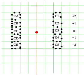
Figure 5: A step in the sweep line algorithm
To do this a sweep line algorithm is used. To compute the Transit Nodes a sweep line is moved across the grid of cells. Instead of focusing on the cell C, this algorithm focuses on potential Transit Nodes. To find all potential Transit Nodes, take all roads that intersect the sweep line and again take the endpoint with the lower id. Let V be the set of all these endpoints. Let CL/R be the set of cells two cells left/right of the sweep line. Then find all boundary nodes vL/R on the boundary of CL/R and for all v in V compute the distances dist(v, vL/R) for all vL/R.
Now that we know alldist(v, vL/R) look at all combinations of vL and vR with a vertical distance of at most 4. For each combination findvso that dist(vL, v) +dist(v, vR) is minimal.
Then v is a Transit Node for the cells thatvL andvR lie in.
After a full horizontal and vertical swipe the complete set of Transit Nodes is computed.
Due to the shortest path queries starting in the middle of the shortest path instead of an endpoint as before the search radius is only about 3 cells wide and the algorithm is faster.
2.5 Computing the distance tables
To finish the preprocessing the distance tables for all distances dist(src, t1) and dist(t1, t2) have to be computed. The former is a trivial modification to the algorithm used to find the set of Transit Nodes that simply stores the results of the shortest path queries for later use.
The latter can be done with an extra APSP step for all Transit Nodes. This is possible in acceptable time because the number of Transit Nodes is small. As a ballpark figure, there are about 10 Transit Nodes per cell in the grid and many Transit Nodes are shared between neighboring cells.
2.6 Shortest distance queries
After the preprocessing has been done, shortest distance queries can be answered using just a few distance table lookups if the trip is ‘far’ enough. To finddist(src, trg) =min(dist(src, t1)+
dist(t1, t2) +dist(t2, trg)) as described in Section 2.2 the number of lookups is almost constant since the number of Transit Nodes per node is low.
2.7 Shortest path queries
For many applications not only the shortest distance but also a full shortest path is needed.
To reconstruct a shortest path start at trgand divide the path into a know and an unknown part with a nodeu in between. At the beginning onlytrg is known andu=trg.
Then gradually always find the next step on the path by checking all adjacent nodes of u to find one such that d(u, src) = d(u, v) +d(v, src). This is fast because with TRANSIT shortest distance queries are fast. But when approaching the src it’s not longer possible to use TRANSIT because the distance between u andsrcis no longer long enough.
If the distance betweensrc and trg is long then it’s possible to reverse the search in this case and restart the algorithm starting atsrcworking backwards. Otherwise another shortest path has to be used to reconstruct the remaining path.
2.8 Local queries
The same problem of too short queries can also occur at other times. To be able to answer all types of queries, not just ‘far’ ones, another shortest path or shortest distance algorithm has to be used.
Fortunately, most other algorithms are fast if the trip is short and there are already many options including Dijkstra’s algorithm and Highway Hierarchies.
It’s obvious that TRANSIT cannot always be used as it depends on a Transit Node lying on a shortest path between srcand trgwhich isn’t always the case for local queries.
2.9 Multi-Level Grid
A problem still unanswered is the question of the grid size. Table 6 shows how different grid sizes affects the performance of the algorithm.
The goal is that as many queries as possible are global and thus fast while keeping the number of Transit Nodes in |T|low.
Size |T| |T| × |T|/node % global queries preprocessing
64×64 2042 0.1 91.7% 498 min
128×128 7426 1.1 97.4% 525 min
256×256 24899 12.8 99.2% 638 min
512×512 89382 164.6 99.8% 859 min
1024×1024 351484 2545.5 99.9% 964 min
Figure 6: Performance of different grid sizes (US road network)
It’s hard to find a grid size that matches these criteria all at once. But instead of using just one grid it’s possible to precompute data for multiple grid sizes and use the right grid for each query.
To do this the precomputation starts with a coarse grid as described above and finer grids then get added afterwards. For the finer grids only query regions that would be local for the coarser grid have to be considered.
For queries then the first action is to find the coarsest grid for which the query is still global and then using this grid with the standard lookup algorithm.
3 Conclusions
TRANSIT allows for almost constant time shortest distance queries on road networks while preprocessing time and space usage isn’t too large. It improves query time by more than a factor of a magnitude from milliseconds to microseconds.
While TRANSIT is focused on road networks it’s possible to adapt this algorithms to other graphs that also exhibit the same channeling characteristic so that it an equivalent of the Transit Nodes can be found.
References
[BFM07] Holger Bast, Stefan Funke, and Domagoj Matijevic. TRANSIT Ultrafast Shortest- Path Queries with Linear-Time Preprocessing, 2007.
[BFM+08] Holger Bast, Stefan Funke, Domagoj Matijevic, Peter Sanders, and Dominik Schultes. In Transit to Constant Time Shortest-Path Queries in Road Networks , 2008.