FLUCTUATIONS IN AND OUT OF EQUILIBRIUM:
Thermalization, quantum measurements and Coulomb disorder I n a u g u r a l – D i s s e r t a t i o n
zur
Erlangung des Doktorgrades
der Mathematisch-Naturwissenschaftlichen Fakultät der Universität zu Köln
vorgelegt von Jonathan Lux
aus Essen
Köln
2016
Berichterstatter: Prof. Dr. Achim Rosch Prof. Dr. Sebastian Diehl
Tag der letzten mündlichen Prüfung: 24.5.2016
Summary
This purely theoretical thesis covers aspects of two contemporary research fields:
the non-equilibrium dynamics in quantum systems and the electronic properties of three-dimensional topological insulators.
In the first part we investigate the non-equilibrium dynamics in closed quantum systems. Thanks to recent technologies, especially from the field of ultracold quan- tum gases, it is possible to realize such systems in the laboratory. The focus is on the influence of hydrodynamic slow modes on the thermalization process. Generic systems in equilibrium, either classical or quantum, in equilibrium are described by thermodynamics. This is characterized by an ensemble of maximal entropy, but con- strained by macroscopically conserved quantities. We will show that these conserva- tion laws slow down thermalization and the final equilibrium state can be approached only algebraically in time. When the conservation laws are violated thermalization takes place exponential in time. In a different study we calculate probability distribu- tions of projective quantum measurements. Newly developed quantum microscopes provide the opportunity to realize new measurement protocols which go far beyond the conventional measurements of correlation functions.
The second part of this thesis is dedicated to a new class of materials known
as three-dimensional topological insulators. Also here new experimental techniques
have made it possible to fabricate these materials to a high enough quality that their
topological nature is revealed. However, their transport properties are not fully un-
derstood yet. Motivated by unusual experimental results in the optical conductivity
we have investigated the formation and thermal destruction of spatially localized
electron- and hole-doped regions. These are caused by charged impurities which are
introduced into the material in order to make the bulk insulating. Our theoreti-
cal results are in agreement with the experiment and can explain the results semi-
quantitatively. Furthermore, we study emergent lengthscales in the bulk as well as
close to the conducting surface.
Deutsche Zusammenfassung
Die vorliegende rein theoretische Arbeit behandelt Aspekte zweier aktueller For- schungsbereiche: die Nicht-Gleichgewichtsdynamik von Quantensystemen und die elektronischen Eigenschaften von topologischen Isolatoren.
Im ersten Teil untersuchen wir die die Nicht-Gleichgewichtsdynamik in abge- schlossenen Quantensystemen. Dank neuartiger Technologien, vor allem im Bereich ultrakalter Quantengase, ist es möglich solche Systeme im Labor zu realisieren. Der Schwerpunkt liegt auf der Untersuchung des Einflusses langsamer hydrodynami- scher Moden auf den Prozess der Thermalisierung. Generische Systeme im Gleichge- wicht könne mittels Thermodynamik beschrieben werden. Diese ist charakterisiert durch ein Ensemble maximaler Entropie, unter Bedingungen die durch makroskopi- sche Erhaltungssätze auferlegt werden. Wir werden zeigen, dass diese Erhaltungs- größen die Thermalisierung verlangsamen, und der finale thermische Zustand nur algebraisch in der Zeit erreicht werden kann. Werden die Erhaltungssätze verletzt, erfolgt die Thermalisierung exponentiell in der Zeit. In einer anderen Studie berech- nen wir Wahrscheinlichkeitsverteilungen von projektiven Quantenmessungen. Neu entwickelte Quantenmikroskope bieten die Möglichkeit neuartige Messprotokolle zu realisieren, die weit über die konventionellen Messungen von Korrelationsfunktio- nen hinausgehen.
Im zweiten Teil der Arbeit widmen wir uns neuartigen Materialien, welche in die Klasse der dreidimensionalen topologischen Isolatoren fallen. Auch hier haben neu- artige experimentelle Methoden dazu geführt, dass diese Materialien in sehr guter Qualität hergestellt werden können und die topologischen Eigenschaften zum Vor- schein treten. Ihr Transportverhalten ist jedoch noch nicht vollständig verstanden.
Motiviert durch ungewöhnliche Messergebnisse in der optischen Leitfähigkeit, ha-
ben wir die Entstehung und thermische Vernichtung von räumlich begrenzten Elek-
tron und Loch-Bereichen in diesen Materialien untersucht. Diese werden verursacht
durch geladene Fremdatome welche ins Material eingebracht wurden um es isolie-
rend zu machen. Unsere Ergebnisse sind im Einklang mit dem Experiment, welches
durch diese Mechanismen semi-quantitativ erklärt werden kann. Des weiteren un-
tersuchen wir emergente Längenskalen in diesen Systemen, sowohl im Inneren, als
auch nahe der leitenden Oberfläche.
Contents
PART I:
Semiclassical dynamics after quantum quenches:
Hydrodynamic long-time tails and projective measurements 1
1 Introduction I 2
2 Ultracold atoms in optical lattices 15
2.1 Producing a lattice for neutral atoms . . . . 15
2.2 Interactions . . . . 17
2.3 Quantum microscopes . . . . 19
2.4 Observing the unitary time evolution . . . . 21
3 Methods 23 3.1 Derivation of effective Hamiltonians . . . . 23
3.2 Lattice scattering theory in 1d . . . . 25
3.3 Quasiparticle momentum distribution . . . . 34
3.4 Semiclassical dynamics after weak quantum quenches . . . . 39
4 Diffusion and fluctuating hydrodynamics 43 4.1 Random Walks . . . . 44
4.2 Fluctuations . . . . 45
4.3 Scaling analysis of the diffusion equation . . . . 50
4.4 Long-time tails . . . . 51
4.5 Violation of the conservation laws . . . . 56
4.6 Mode couplings . . . . 58
5 Hydrodynamic long-time tails after a quantum quench 60 5.1 Diffusive thermalization after weak quenches . . . . 63
5.2 Equilibrium results . . . . 69
5.3 Comparison to the Boltzmann equation . . . . 74
5.4 Exact diagonalization for strong quenches . . . . 76
6 Violation of the conservation laws: Numerical Results 79 6.1 Thermalization in the absence of conservation laws . . . . 80
6.2 Relaxation in the driven system . . . . 82
6.3 Adiabatic limit . . . . 85
7 Quench dynamics and statistics of measurements 90
7.1 Creation of quasiparticles . . . . 92
7.2 Scattering and emission . . . . 94
7.3 Time dependent results . . . . 97
7.4 Characterization of the final ensemble . . . . 100
8 Outlook I 104 PART II: Coulomb disorder in three-dimensional topological insulators 107 9 Introduction II 108 10 The experiment 112 10.1 Optical properties of solids . . . . 114
10.2 Experimental results for the optical conductivity . . . . 115
10.3 Experimental results for the optical weight . . . . 117
10.4 Contribution of the surface states . . . . 119
11 Theoretical description of compensated semiconductors 121 11.1 Doped semiconductors . . . . 121
11.2 The model . . . . 125
11.3 Numerical implementation . . . . 128
12 Low temperatures: Puddles and lengthscales 132 12.1 Coulomb gap . . . . 132
12.2 Correlation functions and lengthscales . . . . 135
12.3 Puddles . . . . 151
13 Puddle destruction at finite temperatures 155 13.1 Thermal screening . . . . 155
13.2 Numerical results . . . . 157
13.3 Comparison to the experiment . . . . 160
14 Including the surface states 162 14.1 Dirac systems . . . . 162
14.2 Screening theory . . . . 163
14.3 Numerical implementation . . . . 168
14.4 Numerical results . . . . 169 14.5 Connection to the bulk lengthscales . . . . 177
15 Outlook II 179
References 180
PART I
Semiclassical dynamics after quantum quenches:
Hydrodynamic long-time tails
and projective measurements
1 Introduction I
Non-equilibrium is the absence of equilibrium. A system in equilibrium is described by thermodynamics, a coarse-grained theory which only has the macroscopically con- served quantities of the system as degrees of freedom. The density matrix is of a universal form. Its structure is determined by having the highest entropy consis- tent with the values of the conserved quantities. Equilibrium is accompanied by a temporal invariance and expectation values are said to be time-independent. How- ever, expectation values of non-conserved quantities fluctuate on microscopic scales.
A macroscopic description is implicit in the notion of equilibrium. On the coarse- grained scales, correlations between different times depend only on the time differ- ence.
Out of equilibrium this is in general not the case. Exceptions include non-equi- librium steady states. For example, externally driven systems can show a steady current flow. By contrast, in equilibrium the (average) current is zero. Due to the more complex temporal structure of non-equilibrium systems it is generically harder to describe these theoretically as compared to equilibrium systems. We start by intro- ducing some terminology inherent to modern non-equilibrium quantum mechanics.
Closed quantum systems. In theoretical approaches to condensed matter systems it is (almost) always assumed that the system of interest is in thermal equilibrium.
A coupling to an environment is implicitly assumed. The many degrees of freedom of the environment enter the description only via their statistical properties, for ex- ample via the temperature. If the environment is in equilibrium, and is much larger than the system of interest, it is called a
bath. The Hilbert space of the total systemis
H=
Hsystem⊗ Henvironmentwhere
⊗denotes the tensor product. If the degrees of freedom of
Henvironmentare traced out the dynamics in
Hsystemis not unitary any more.
Furthermore the state of the system has to be described as a mixed state, in contrast to the state of the full system which might be a pure state. In this approach also the energy stored in the degrees of freedom of
Hsystemis not necessarily conserved any more. We will refer to this subsystem as an
open (quantum) system.We will consider the dynamics in
closed quantum systems. They are defined by theproperty that they are isolated from their environment and are described by a time-
independent Hamiltonian. This implies that the time evolution is unitary and that
the energy is conserved. It is obvious that the closedness of a system, if it is not the
full universe, can only be an approximation. However, in many experiments closed-
ness is a decent approximation. In particular in recent years new techniques have allowed experimentalists to realize quantum systems which are effectively closed on the timescales of the experiments. These systems are, among others, ultracold atoms in optical lattices. We will introduce them in the next section in more detail. Often these systems are well described by Hamiltonians known from condensed matter sys- tems, like Hubbard models or Heisenberg models. The reason is that in both systems the relevant (low-energy) degrees of freedom are interacting particles in a periodic potential. While typical condensed matter are performed at temperatures between 10
−3K (
3He/
4He dilution refrigerator) and room temperature, ultracold atom exper- iments are performed at temperatures 10
−9−10
−4K.
In condensed matter systems the periodic potential is provided by the atomic nu- clei. There collective low-energy excitations, phonons, are often assumed to be in equilibrium. They provide the aforementioned bath for the electronic and/or mag- netic degrees of freedom. In optical lattices neutral atoms are trapped in periodic laser potentials. Regimes can be reached where there is no energy exchange between the atom and laser degrees of freedom. Therefore the atomic system can often be con- sidered as closed on the experimental timescales. However, other processes restrict these timescales, for example atom losses.
In contrast to condensed matter systems, in optical lattice experiments the mi- croscopic parameters can be tuned, among them are dimensionality, lattice structure and the interaction strength, exploring new regimes which are not realized in con- densed matter systems. Furthermore quantities which are inaccessible in condensed matter systems can be measured. Quantum microscopes, for example, can resolve positions of individual atoms with single site precision. Due to the high control over the microscopic parameters also new experimental protocols can be realized.
Quantum quenches. In a quantum quench a parameter in the Hamiltonian is changed on very short timescale. If this is done fast enough, on a timescale smaller than all intrinsic timescales of the system, the quantum state does not change. This is in contrast to an
adiabaticchange of parameters. If the change of the parameter is performed very slowly, on a timescale much larger than all intrinsic timescales, the system remains in its time-evolving eigenstate if there are no energy crossings.
This is the statement of the
adiabatic theorem. Since in a quantum quench the timeevolution operator is changed, but the quantum state is not, dynamical processes
are induced. This is the case even if the system was in an equilibrium state, for
example in the groundstate, before. The most-studied protocol, at least theoretically,
of a quantum quench is the following
1:
(QQ1) Prepare the system in the groundstate of a Hamiltonian H(J ˆ
ini).
(QQ2) Instantaneously change J
ini→J
finalto obtain the Hamiltonian H(J ˆ
final) = ˆ H
f. (QQ3) Study the time evolution of an observable
hOi(t) ˆ with the new Hamiltonian H ˆ
f.
As the system was in the groundstate before the quench, but it is not afterwards, this can be viewed as a well-defined way to pump energy into the system. The problem of a quantum quench can formally be solved easily:
(SQ1) Diagonalize the final Hamiltonian H ˆ
f|ni= E
n|ni.(SQ2) Decompose the initial state into the eigenstates
{|ni}of H ˆ
f:
|inii=
Pn
c
n|ni.(SQ3) Calculate the unitary the time evolution for t > t
inias
|ti
= e
−iHˆf(t−tini)|inii=
Xn
c
ne
−iHˆf(t−tini)|ni=
Xn
c
ne
−iEn(t−tini)|ni. (1.1)
(SQ4) Evaluate the observable of interest as (we use t
ini= 0)
hOi(t) = ˆ
ht|O|ti ˆ =
Xn,m
c
∗mc
ne
i(Em−En)tO ˆ
mn=
Xn
|cn|2
O ˆ
nn+
Xn6=m
c
∗mc
ne
i(Em−En)tO ˆ
mn. (1.2)
In practice one already fails at step (SQ1). Here an exponentially large (in the num- ber of particles) matrix has to be diagonalized. One can make use of symmetries, if present, to block-diagonalize H ˆ and in this way split the problem into smaller pieces.
But nevertheless in general it is a hopeless task. It is possible to use brute-force nu- merical exact diagonalization methods (ED) to perform the scheme described above.
But for interacting systems this is restricted to a small number of particles, typically 10
−20 on present day computers. Nevertheless it can be very useful. For short times one can use time-dependent perturbation theory. But also here the complexity grows exponentially with the order of perturbation theory.
1Throughout this thesis we use~ = 1. Then the unit of energyEis equal to the unit of frequency ωand the unit of momentapis equal to the unit of1/length= 1/l. The dimensions can be restored by E =~ωandp=~/l. We will reintroduce~only for dimensional considerations. Furthermore we use the common notation that operators acting on the Hilbert spaceHare denoted with a hat on top, for exampleHˆ denotes the Hamilton operator. In addition we use the braket notation for quantum states as introduced in standard textbooks of quantum mechanics. Matrix elements of an operatorOˆin a basis {|ni}are denoted byhm|O|niˆ = ˆOmn. In continuous systems the sums have to be replaced by integrals.
ˆ
The formal solution, Eq. (1.2), does not really give any physical insight. In equi- librium, mean field theories and renormalization group schemes are very successful in identifying the relevant (low-energy) degrees of freedom. Nothing like this seems to be within reach here. Non-equilibrium field theory methods are often needed to make any progress [1–3].
In recent years time-dependent extensions of sophisticated numerical methods have been developed: most prominently, the non-equilibrium dynamical mean field theory (NEQ-DMFT) [4], and the time-dependent density matrix renormalization group (t-DMRG) [5]. Both are tailored to a certain class of models. DMFT is a self- consistent method for lattice models. The decisive approximation is the locality of the self energy. This approximation is better the higher the dimension or, more pre- cisely, the larger the coordination number of the lattice. DMRG methods are only applicable for 1d systems or 2d systems in a rod geometry. In the modern formula- tion DMRG works with matrix product states, which can only partially capture the entanglement growth in generic non-equilibrium systems. Therefore the time range in which reasonable results are obtained is restricted.
From Eq. (1.2) one can see that the expectation values of conserved quantities are time-independent. A conserved quantity is defined by the property that the corre- sponding operator C ˆ commutes with the Hamiltonian: [ ˆ C, H] = 0. Then the eigen- ˆ states of C ˆ are also eigenstates of H ˆ and the second term in Eq. (1.2) vanishes. The result is
hCi(t) = ˆ
Pn|cn|2
C ˆ
nnand independent of t. For example, the expectation value of the energy is
hHi(t) = ˆ
Pn|cn|2
H ˆ
nn=
Pn|cn|2
E
n.
Integrability. An exceptions to the failure of step (SQ1) are
integrablemodels. Here
the
Bethe ansatz[6–9], a unitary transformation to a non-interacting model [10] or
bosonization [11] allows one to diagonalize the Hamiltonian. In some cases it is even
possible to analytically calculate the time dependence of observables after a quan-
tum quench [12–19]. The hallmark of integrability is the existence of a macroscopic
number of
localconservation laws, called charges or constants of motion. Often this
is the case in one dimensional models with short-ranged interactions. For example,
the Heisenberg XXX [6] and XXZ chain [20], the transverse field Ising model [10],
the Fermi Hubbard model [21, 22], the Luttinger liquid [11, 23], the Kondo model
[24] and the Lieb-Liniger model [25, 26] are integrable in one dimension. They have
been solved (diagonalized) in the respective references given above. In this mod-
els the dynamics is highly constrained as the initial expectation values of all the
conserved charges cannot change during the time evolution. By contrast, generic
models only have a small number of conserved quantities related to the fundamental symmetries. Therefore integrable models cannot be described by conventional ther- modynamics. Rather their stationary properties are described by generalized Gibbs ensembles (GGEs) [27, 28]. Here all the conserved charges have to be included into the density matrix.
From Eq. (1.2) it can be directly seen, with the projection onto the eigenstates O ˆ =
|ni hn|, that there are always as many conserved quantities as the dimensionof the Hilbert space. The addition local is essential. Here locality means that the conserved quantity can be written as a sum over a density which has its support on a finite number of lattice sites. Well-known examples include the energy, as a sum over the energy density, and the particle number, as a sum over the particle density. In general it can be very hard to find all conserved charges. It has also turned out that in some models quasi-local charges exist and are important to understand the dynamics [29]. For lattice models quasi-locality means that the corresponding density cannot be defined on a finite number of lattice sites but has exponential tails. Non-interacting models also have a macroscopic number of conserved quantities: the individual one- particle quantum numbers.
For real systems integrability can only be an approximation. Almost any ad- ditional term in the models mentioned above breaks the integrability, for example adding longer-ranged interactions. However, many recent experiments can be de- scribed by integrable models [30–35]. On the timescales of the experiments the dy- namics is effectively integrable.
Another approach to distinguish integrable from non-integrable models is based on random matrix theory. It is known that the level spacing distribution of generic random matrices is described by Wigner-Dyson statistics [36]. The probability to find two subsequent eigenstates with a (normalized) distance s is P
generic(s)
∼s
βe−γs2. β > 1 and γ > 0 depend on the symmetry class. In either case the probability to find eigenvalues very close in energy, s
→0, vanishes. In contrast to that, in integrable models a state does not "feel" the presence of the other states and the eigenvalues are uncorrelated. This leads to a Poisson distribution of the level spacings P
integrable(s)
∼ e−γs[37].
Equilibration. A further observation can be made from Eq. (1.2): if
hOi(t) ˆ ever reaches a time-independent value, it can only be
Pn|cn|2
O ˆ
nn. Only if there are de-
generacies in the spectrum, the second term in Eq. (1.2) can yield a time-independent
contribution. But for generic systems we do not expect any degeneracies (in a sec-
tor with fixed particle number and, possibly, total momentum or magnetization).
The reason is level repulsion: as described above the probability distribution of the level spacings in non-integrable models is
∼s
β>1e−γs2. The probability to have degeneracies s
→0 is zero. Therefore, we expect for non-integrable models that
hOi(t) = ˆ
Pn|cn|2
O ˆ
nn+ F
iniˆO
(t) where F
Oˆhas no time-independent term, and the su- perscript "ini" indicates that F depends on the initial state, see Eq. (1.2). A possible definition of equilibration is that for all initial states and all reasonable observables O, to be specified below, ˆ
F
iniˆO
(t) =
Xn6=m
c
∗mc
ne
i(Em−En)tO ˆ
mn −→t→∞
0. (1.3)
For finite systems, as for example simulated in ED, this definition can never be ful- filled. There are finite size corrections which lead to fluctuations on the right hand side. A pragmatic way is to take the definition in the thermodynamic limit. Further- more there are
quantum revivals[38, 39]. If there is only a finite number of eigen- states the right hand side of Eq. (1.2), it is a sum of finitely many periodic terms.
Then, for mathematical reasons, F
iniˆO
(t) returns arbitrarily close to its initial value during the time evolution. However, for generic systems this happens only on very long time scales. Following [40], the time evolution in a Hilbertspace of dimension N can be visualized by N clocks representing the phases φ of the individual eigenstates.
The probability to find a specific configuration, for example the initial one, within a precision ∆φ is
∼(
∆φ2π)
N. The recurrence time of the full wavefunction is then R
∼(
∆φ2π)
−N/ω where ω is the typical angular velocity – the energy. For
∆φ2π= 0.01 and ω = 1eV
∼1.52
×10
15sec
−1R exceeds the age of the universe already for N = 17.
Nevertheless observables can show recurrences at smaller times but for macroscopic systems they are usually not of any relevance. Exceptions in a many particle system can occur in Bose Einstein condensates where the phases are locked [41].
Eq. (1.3) depends on the observable O, which means that some observables can ˆ equilibrate while others do not. This is generically the case; for example, the energy does always equilibrate in this sense. But let us consider the operator O ˆ
ab=
|ai hb|+
|bi ha|
where
|aiand
|biare eigenstates with E
a−E
b= ω
ab 6= 0and c
a, c
b 6= 0. ThenO ˆ
abdoes never equilibrate.
The definition, Eq. (1.3), is only useful for
measurablequantities. A broad class of measurable observables are local. Again, locality means that it can be written as a sum of local terms: O ˆ
local=
Pj
O ˆ
jwhere O ˆ
jhas support (is non-zero) only
in a small region of space. In lattice models it must have support only on a small
number of connected lattices sites. A prime example is the total magnetization in lattice spin models: M ˆ =
Pj
σ
zj. Thanks to linearity of the time-evolution, it is F
iniˆOlocal
(t) =
Pj
F
iniˆOj
(t). Then all parts O ˆ
jequilibrate independently and the rest of the system can serve as an environment. One can decompose the Hilbertspace as a tensor product
H=
⊗jHj. The measurement is then performed only in one sector
Hjand the result is averaged over j. Higher order correlation functions include more sectors. As long as the number of involved sectors is much smaller than the particle number, the rest of the system can still serve as an environment.
An important quantity which does not fall into this class is the occupation of the momentum modes n ˆ
k. It can be accessed in time of flight measurements [42–44].
The equilibration of n ˆ
kimplies
detailed balance. The transition rate into the single-particle state
|kihas to be equal to the transition rate out of
|ki. We will show furtherexamples for the measurement of distribution functions in the next section.
Prethermalization. Some systems show an emergent integrability on short time- scales –
prethermalization[45]. In this regime expectation values of observables show prethermalization plateaus which means that they are time independent for some time [46, 47]. But these values are not consistent with the thermal values. Only at later times the non-integrability eventually leads to true thermalization. Many nu- merical studies, for example [46, 48], and recent experimental studies, for example [32, 49], have investigated this regime. The quasi-stationary properties can be de- scribed by generalized Gibbs ensembles as in integrable systems. To be precise, all real world manifestations of integrable models are in the prethermalized regime. As aforementioned integrability can only be an approximation for real systems, which are then rather described as prethermalized.
Irreversibility. The microscopic equations underlying the dynamics, either quan- tum or classical, are time-reversal invariant. This is seemingly in contradiction to the second law of thermodynamics: it states that the entropy (almost) always in- creases, thereby distinguishing the two time directions. The system spontaneously
"finds" its highest entropy state – the equilibrium. If the system of interest is coupled to a bath, it is plausible that the equilibrium, and thereby the time direction, in the subsystem is externally imposed. But what about closed systems?
Irreversibility requires a coarse-grained point of view. Formally, this is achieved
by distinguishing microstates and macrostates. In a microstate all degrees of free-
doms of the system are specified. In classical physics this corresponds to one point in
phase space, and in quantum mechanics this implies a knowledge of the full wave- function or density matrix. This cannot be measured let alone experienced by the sensory organs. A macrostate is obtained by fixing the (average) values of some ob- servables. This defines a probability distribution – an
ensemble– as a macrostate is compatible with many microstates. In quantum mechanics, an ensemble is described by a mixed state and represented in terms of a density matrix. In this description the observables which are taken into account and all other degrees of freedom play a very different role. The fact that the microstate is not specified leads to fluctuations on microscopic scales.
In thermodynamics only the (average) values of macroscopically conserved quan- tities are specified. Usually these are the energy and the particle number. The corre- sponding thermodynamical ensemble is defined by having the largest entropy among all ensembles consistent with the given values. This is the fundamental assumption of statistical mechanics. Experience shows that this is often sufficient to describe ex- perimental results. The entropy of a probability distribution P =
{p1, p
2, ...|
Pj
p
j= 1} (a density matrix ρ) is defined as ˆ
S(P ) =
−Xj
p
jlog(p
j) (S( ˆ ρ) =
−T r( ˆ ρ log( ˆ ρ))) . (1.4)
Under reasonable assumptions (most importantly additivity) the structure of the for- mula given above can be uniquely determined, see for example [40]. The prefactor has to be fixed by convention or normalization. The entropy is a measure for the lack of information. The maximum entropy assumption and the second law of thermody- namics then state that the time direction is fixed by the loss of information. This is, of course, not the full story. Most importantly broken symmetries are ubiquitous on all scales from particle physics to cosmology. By contrast, thermodynamic ensembles respect the symmetries of the system, see for example the famous article "More Is Different" by P. W. Anderson [50].
If a system can be locally described by a thermodynamic ensemble, a hydrody- namic description is appropriate. Here "locally" refers to a scale which is much smaller than the system size but much larger than any correlation length or mean free path. Then one can specify the time and space dependent temperature T (r, t) or, equivalently, the energy density e(r, t). The same holds for the densities of other con- served quantities. If one chooses a coarse-grained, thermodynamic or hydrodynamic, description of the system the fluctuations can be described only statistically.
It is common to refer to the equilibrium ensemble as the equilibrium state. We
will also use this terminology, however, one has to keep in mind that this refers to a probability distribution rather than to a (micro-)state.
A simple picture for irreversibility arises if one assumes that the dynamics is ergodic. Ergodicity means that during the time evolution with the microscopic equa- tions the full available phase space is covered equally. Then, if the system is ini- tialized in an atypical (=non-equilibrium) state, thermalization is just a matter of probabilities. For concreteness let us consider a classical closed system in which en- ergy and particle number are conserved. Thermodynamically, this is described by a microcanonical ensemble where all microstates consistent with the given energy and particle number are equally probable. This probability distribution has the largest entropy among all possible distributions. Seemingly there are no atypical states.
However, from a coarse-grained perspective this is not true. We consider an over- simplified, yet very instructive, standard example: N = 10
23molecules in a box. We assume that the probability for a distinguished particle to be in the left half of the box is 1/2. We further assume that, independent of the energy, the number of available microstates in the macrostate
{N1, N
2= N
−N1}is
NN1
. Here N
1denotes the number of molecules in the left half and N
2denotes the number of molecules in the right half.
We focus on a description with these macrostates giving a coarse-grained picture. We totally omit the energy conservation for conceptual clarity. And, obviously, quantum statistics is different.
The probability to find all the particles in one half of the box is
∼2
−1023. This number is so ridiculously small that one would need billions of terabytes to store its digits
2. From the macroscopic point of view it is reasonable to call this an atypical state. The notion of equilibrium itself requires a coarse-grained, macroscopic, point of view. Otherwise it is not possible to distinguish typical from atypical, equilibrium from non-equilibrium, configurations. In practice an atypical state can be realized by connecting a ultrahigh vacuum chamber to a normal gas. If we release such a system it is intuitively clear that after some time the number of molecules in both boxes will be approximately the same (if they are of equal size). But we will never find that a macroscopic ultrahigh vacuum region emerges spontaneously. From the macroscopic point of view the process is irreversible. To produce an ultrahigh vacuum chamber requires a high effort and sophisticated technology. A non-equilibrium state is a highly fine-tuned state.
In equilibrium there will be fluctuations in the number of molecules per box. As- suming equal sized boxes and ergodicity, the expectation value per box is µ = N/2.
2It is:1023bits∼1022bytes∼1019KB∼1016MB∼1013GB∼1010TB
The typical fluctuations are given by the square root of the variance of the corre- sponding probability distribution. The probability to find M excess molecules in the left or the right box, a macrostate
{N/2 +M, N/2
−M} or
{N/2−M, N/2 + M
}, isP
±M= 1 2
N
N
N 2 ±
M
= 1 2
NN !
N 2
+ M
!
N2 −M
!
≈
1 2
N√
2πN
NeNp
4π
2((N/2)
2−M
2)
N2+M e
N
2+MN
2−M e
N 2−M
= 1
p
2π(N/4
−M
2/N )
eNlog√ N
N2−4M2 eMlog
N−2M
N+2M ≈
1
pπ
2
N
e−2M2
N
, (1.5) where we have used Stirling’s formula in the second line. The final result, valid in the limit N M , is just a Gaussian distribution with variance σ
2= N/4. Thus the typical number of excess molecules in one of the boxes is σ =
√N /2: this describes the thermal fluctuations.
Note that we have not used the notion of time yet. By means of the ergodicity as- sumption, the temporal average is replaced by an ensemble average. The fluctuation formula, Eq. (1.5), is valid on large timescales. We can fix a macrostate at some in- stant of time by reintroducing the barrier and thereby cutting the box in half. We will find a macrostate
{N/2 +M
1, N/2
−M
1}with probability P
M1. If we again release the barrier, say at time t
1, we can ask "What is the typical number of excess molecules M
2at time t
2> t
1?". This is an example of an unequal time correlation function and the answer depends only on ∆t = t
2 −t
1. It is clear that M
2(∆t
→0) = M
1and M
2(∆t
→ ∞) = 0. In formulating the question we have implicitly defined anon-equilibrium ensemble. At t
1only microstates compatible with the macrostate
{N/2 +M
1, N/2
−M
1}are allowed and this is not the ensemble with the highest entropy consistent with N molecules.
Averaged over all possible
{N/2 +M
1, N/2
−M1}macrostates at t
1, with the corre- sponding probability, one obtains the equilibrium unequal-time autocorrelation func- tion
hM(t
1)M(t
2ieq. Its equal time value is
PM
M
2P
M ≈σ
2= N/4. In diffusive systems functions of this type show algebraic long-time tails. If not averaged over all M
1, a non-equilibrium initial condition, they also dominate the thermalization process at late times.
Also in finite classical systems, due to mathematical reasons, the system will come
back arbitrarily close to its initial configuration as described by the Poincaré recur-
rence theorem [51]. However, the recurrence time for a system of 10 or 20 particles
is again much larger than the age of the universe [52]. Thus it does not have any physical consequences for macroscopic systems.
The initial states in quantum quench setups are very often low entanglement states. Groundstates of gapped Hamiltonians, often chosen as initial states, show area laws for the entanglement entropy [53]. Often product states are chosen. Only the high effort of the experimentalists to prepare such an atypical state, by lowering the entropy using sophisticated cooling schemes, make it possible to investigate the non-equilibrium. Theorists don’t care since product states are easily written down and can be nicely depicted. We will make use of this later.
All processes taking place in nature are accompanied by an entropy growth (re- ferred to as friction or heating), an unavoidable consequence of the tendency to ther- malize – or statistics. Even if it would be possible to microscopically change the time direction (for example by letting H ˆ to
−H ˆ in a quantum system), the tiniest perturbation, which is unavoidable in practice, will hinder system to go back to its initial non-equilibrium state. Only if the non-equilibrium is artificially maintained, for example by driving, the (sub-)system can be prevented from going to equilibrium.
Exceptions can arise in highly inhomogeneous systems as further discussed below.
Thermalization. Eq. (1.2) can also be written in terms of a density matrix ρ
QQ(t) as
hOi(t) = Tr ˆ
O ρ ˆ
QQ(t)
. The time-independent part is called the
diagonal ensemble,its density matrix ρ ˆ
DEis defined by
ˆ
ρ
DE=
Xn
|cn|2|ni hn|
, then
Xn
|cn|2
O ˆ
nn= Tr
O ˆ ρ ˆ
DE. (1.6)
ˆ
ρ
DEdepends on all the details of the initial state via the macroscopically many num- bers c
n. This is in vast contrast to the equilibrium density matrix ρ ˆ
eq, which only depends on a very small number of parameters. The full density matrix after a quantum quench can never become a thermal density matrix. The density matrix of the canonical ensemble ρ ˆ
can=
exp−β
H ˆ
/Z
candepends only on one parameter, the temperature T , or, equivalently, its inverse β = 1/T (we use k
B= 1 throughout).
Z
can= Tr
exp
−β
H ˆ
denotes the canonical partition function. A possible defini- tion of thermalization might be the following: a quantum system thermalizes if for all measurable observables O ˆ and all initial states:
Tr
O ˆ ρ ˆ
DE= Tr
O ˆ ρ ˆ
eq(T, . . . )
. (1.7)
This implicitly defines the temperature T and possibly other, but only very few, pa-
rameters (fixed by the few macroscopically conserved quantities) as indicated by the dots. Again, the definition has to be understood modulo finite size effects and quan- tum revivals. According to the definition integrable models do not thermalize as they have many conserved quantities. But they can, and often do, equilibrate.
Another class of interacting systems which fail to thermalize are many-body lo- calized systems [54, 55]. While in non-interacting disordered systems the single- particle states are, completely or partially (depending on the dimensionality) local- ized [56, 57], many-body localization is a complex interplay of disorder and interac- tions. First experiments have been reported recently [58, 59].
A widely accepted mechanism which leads to thermalization in closed quantum systems is the
eigenstate thermalization hypothesis(ETH) [60, 61]. The essential as- sumptions are that 1) the diagonal matrix elements O ˆ
nn= O(E
n) depend smoothly on the energy and that 2) the off-diagonal matrix elements O ˆ
m6=nare typically much smaller than the diagonal elements:
|O ˆ
m6=n| |O ˆ
nn|. If we assume that the distri-bution of the energies is confined to the interval I
hHˆi,∆E= [h Hi − ˆ ∆E/2,
hHi ˆ + ∆E/2]
containing
NhHˆi,∆Estates, we obtain from Eq. (1.2)
hOi(t) ˆ
−→t→∞
X
n
|cn|2
O ˆ
nn+
Xn6=m
c
∗mc
ne
i(Em−En)tO ˆ
mn≈X
n
|cn|2
O(E
n)
≈1
NH,∆EˆX
E∈IhHi,∆Eˆ
O(E). (1.8)
The last formula is exactly the definition of the microcanonical ensemble. For ∆E
→0 the result is just
hOi(t) ˆ
−→t→∞
O(h Hi), and only depends on one number: the expectation ˆ value of the energy
hHi. In this way the universal regime of thermodynamics can be ˆ recovered. Since the result does not depend on the eigenstate that is picked out of I
hHi,∆Eˆ, provided that ∆E is small enough, this implies that each eigenstate is intrinsically thermal. A numerical study and further details on the ETH can be found in [62]. The ETH suggests a mechanism how thermalization arises in quantum systems. Following [62], in the initial state the thermal properties are hidden by fine- tuned phases of the contributing eigenstates. During the time evolution the different eigenstates dephase and, eventually, reveal their thermal nature. However, a full theory of quantum thermalization is not available at present.
In either case, quantum or classical, the non-equilibrium to equilibrium transition
is unavoidable and is irreversible on all reasonable timescales. There are exceptions
in inhomogeneous systems: either if the Hamiltonian itself is highly inhomogeneous,
for example in systems showing many-body localization, or if the initial state is inho-
mogeneous. In the latter case the system can fail to thermalize in the thermodynamic limit. Consider, for example, the two boxes as above one filled with a gas of molecules the other initially empty. If we, hypothetically, increase the size of both boxes to an infinite volume, it is obvious that in the box which was initially empty there are al- ways regions that are still empty. If the maximal velocity of the molecules is c, then regions which have a distance larger than ct from the former barrier cannot contain any molecule. Therefore, the density can never become homogeneous and the sys- tem fails to thermalize. This can be easily extended to quantum systems, where a maximal velocity is provided by Lieb-Robinson bounds [63].
Our work. We will consider two different quantum quenches which, in principle, can be realized with ultracold atoms in optical lattices.
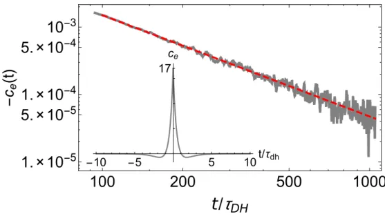
In the first study we will investigate the bottleneck for thermalization in diffusive homogeneous system: the build-up of thermal fluctuations. While many theoreti- cal approaches predict an exponential decay towards equilibrium, we find only an algebraic decay. We will describe the thermalization on a coarse-grained scale by fluctuating hydrodynamics. This generically leads to long-time tails. If we accept that quantum systems thermalize, we also have to accept that – close to equilibrium – they are described by hydrodynamics. As an example to demonstrate this, we will investigate the 1d bosonic Hubbard model. We will find that numerical results are in perfect agreement with predictions from hydrodynamics and linear response theory.
Some of the results can be found in the publication [P1].
In a second study we will calculate the full distribution function of an observable.
In conventional experiments only, usually first or second, moments are measured.
The new experimental techniques make it possible to go beyond this. We will consider the fragmentation of a spin line into bound states. We will calculate the bound state distribution which arises as a result of projective quantum measurements. The model we use is the XXZ Heisenberg model. The results can be found in the publication [P2].
As a preparation, we will introduce the experimental systems we have in mind
and the methods we have used in the next two sections. This is followed by a section
on fluctuating hydrodynamics and diffusion.
2 Ultracold atoms in optical lattices
The field of ultracold quantum gases has offered a lot of trend-setting experiments during the last years and no doubt there are still more to come. Many review arti- cles are available by now, we have mainly used [43, 44, 64–67] for the foundations presented below.
At the present day, temperatures as low as
∼10
−9K for bosons [68] and
∼10
−5K for fermions [69] can be realized in experiments. To reach these ultralow temper- atures, sophisticated cooling schemes have been developed [64, 70, 71]. In experi- mental systems usually alkali atoms are used, having only a single valence electron.
Depending on the number of neutrons they can be either bosonic (B) or fermionic (F). The most commonly used atoms are
87Rb (B),
23Na (B),
7Li (B),
6Li (F) and
40K (F) [66]. Also the trapping of monoatomic [72] and diatomic [73] molecules has been reported.
We will focus on trapping neutral atoms with optical dipole traps. Alternatives include the trapping by inhomogeneous magnetic fields [74, 75]. Another related field is the realm of trapped atomic ions [76, 77].
2.1 Producing a lattice for neutral atoms
The reason that neutral alkali atoms can be trapped with laser light is that they have a simple dipole transition from nS (l = 0) to nP (l = 1) where l denotes the an- gular momentum quantum number and n the principal quantum number. For Alkali atoms, the energy difference is ω
0= 1.5−2eV , corresponding to a photon wavelengths of 1600
−1200 nm. For simplicity, let us consider a toy atom that only has these two states, denoted by
|0iand
|1i. Furthermore we assume only two constituents: a pos-itive nucleus+core electrons, kept fix at a position
Rwith total charge +|e|, and a negative valence electron with charge
−|e|. Although this is of course oversimplified,it captures all the relevant physics and is a decent approximation for alkali atoms at low energies.
In second order perturbation theory, the energy shift of the groundstate in a
static electric field
Eis given by α =
| h0|ˆd·E|1i |2/ω
0. Here
ˆd= e( ˆ
re −R)de-
notes the dipole operator and α is the static polarizability. Laser fields are oscil-
lating with a frequency ω. We denote the corresponding electric field by
E(r, t) = E0(r) 2 cos (ωt) = ˆ
eE
0(r) 2 cos (ωt). The oscillating field induces an oscillating dipole
moment
p= ˆ
ep(r)2 cos (ωt) in the atom. Its amplitude is given by p(r) = α(ω)E
0(r)
where α is the dynamic polarizability, which depends on the laser frequency ω. The
induced dipole moment gives rise to an effective interaction potential for the atom [65]
V
dipole(r) =
−12 hp·Eit=
−12Re (α(ω))
|E0(r)|
2. (2.1) Here
h·itdenotes an average over the rapidly oscillating terms, it arises as the time- scale of the atom motion is much larger than 1/ω.
|E0(r)|
2= I(r) is the intensity of the laser field. The potential leads to a force
F=
−∇Vdipole(r) =
12Re(α(ω))∇I(r).
The polarizability can be calculated to be [65]
α(ω) = 2ω
0ω
20−ω
2−i(ω
3/ω
02)Γ
h0|ˆd·e
ˆ
|1i2
where Γ = ω
033πε
0c
2
h0|ˆd·e
ˆ
|1i2
(2.2)
is the decay rate of the excited state. In the experimentally relevant regime [44]
Γ
|∆|ω
0where ∆ = ω
−ω
0is the
detuning, it follows that Re(α(ω))
≈−
h0|ˆd·e
ˆ
|1i2
/∆ =
−3πε0c2ω30 Γ
∆
and thus
V
dipole(r) =
h0|ˆd·e
ˆ
|1i2
2∆ I(r) = 3πε
0c
22ω
30Γ
∆ I (r). (2.3)
A spatially varying intensity provides a trapping potential for the atoms. Depending on whether the laser is red detuned (∆ < 0) or blue detuned (∆ > 0), the atoms can be attracted or repelled from the intensity maxima. The decay rate Γ limits the lifetime of the experimental system. Absorption of a single photon, with an energy
∼
eV , heats the system up considerably. In the same limit considered above, the atom-photon scattering rate is given by Γ
sc=
3πε2ω03c20
(
∆Γ)
2I (r) such that Γ
sc=
∆ΓV
dipole. Typical experimental values are
∆Γ ∼10
−6[66], which guarantees that there is no energy exchange between the atoms and the laser system on a reasonable timescale.
If I(r) is periodic in space, the laser forms a periodic potential for the atoms. This can be reached by interference of counter propagating laser beams: the potential is then given as V
dipole(r) = V
0(sin
2(k
xx) + sin
2(k
yy) + sin
2(k
zz)). In addition, an harmonic trapping potential is used to prevent the atoms from leaving the lattice. By using different trappings in different directions, the motion of the atoms can effectively be confined to two or one spatial dimension.
The typical energy of an optical lattice is the
recoil energyE
r=
~22m
2λ
2(2.4)
where λ is the wavelength of the laser and m is the mass of the alkali atom. For
typical experimental values (λ = 1000 nm and m = 85u for an Rb atom), the recoil energy is
≈10
−11eV
∼10
−7K
∼2 kHz. If the intensity of the laser is high enough, the atoms are confined to the potential minima (or maxima). The natural description of such a system at low energies is a lattice model using Wannier functions. The tunneling amplitude, or hopping strength, between the minima depends on the depth of the optical lattice V
0. It can be tuned in experiments. Tunneling to non-nearest neighbor sites is highly suppressed and lattice models with only nearest neighbor (nn) hopping provide a very good approximation [44]. In the limit V
0E
r, the nn- hopping amplitude J is approximately given by [44]
J
≈4
√
π V
0E
r 3/4e−2
√
V0/Er
E
r. (2.5)
In the Wannier basis, this leads to the hopping Hamiltonian H ˆ
0=
−J Xhi,ji
ˆ b
†iˆ b
j(2.6)
where i and j label the lattice sites and
hi, jiindicates only nn-hopping.
2.2 Interactions
Optically trapped neutral atoms interact via van der Waals interactions due to the induced dipole moments. We will focus on two-particle scattering here. At large distances r > r
c, where r
cis an atomic lengthscale (∼ nm), this decays as
−C6/r
6with C
6> 0. The van der Waals interaction defines a lengthscale a
c= (2m
rC
6/
~2)
1/4r
cwhere m
ris the reduced mass.
Two-particle scattering only depends on the relative coordinates and can therefore effectively be described by one-particle potential scattering. In 3d scattering theory, the outgoing wavefunction can be decomposed into parts having different rotational symmetry. They are distinguished by the angular momentum quantum number l.
The isotropic part (l = 0) is called s-wave scattering, the l = 1 part is called p-wave scattering, etc. , as in the labeling of atomic orbitals. The energy of the l > 0 channels is separated from the s-wave channel by an energy R
c ∼~2/(m
ra
2c). Typical experi- mental values are R
c ∼mK and if T R
cthe l > 0 channels are effectively closed and only s-wave scattering is relevant, or open. This can be taken as the definition of the regime of ultracold atoms [44]. The s-wave scattering at low energies can be parametrized by a single parameter, the scattering length a
s ∼a
c. The corresponding scattering amplitude for radial momentum k is given by f (k) =
1+ika−ass
. This is the
exact result for a pseudopotential V
pseudo(r) =
4π2m~2asr
δ(r) = gδ(r). However, the regu- larization of the δ-function can cause problems [44, 66]. The important result is that the effective interaction is short-ranged and parametrized by a single parameter a
s. For indistinguishable fermions there is no s-wave scattering due to anti-symmetry.
At low energies, ka
s1, they are effectively non-interacting.
In the pseudopotential approximation, the interaction between bosons is H ˆ
int=
g2Z
d
3rˆ b
†rˆ b
†rˆ b
rˆ b
r. (2.7) In the Wannier basis used for the lattice description this corresponds to an on-site interaction U . In the limit V
0E
r, this is given by [44]
U
≈ r8
π a
sl V
0E
r3/4
E
r, (2.8)
where l is the lattice constant. In combination with the hopping term, Eq. (2.6), this leads to the bosonic Hubbard model
H ˆ
BH=
−J X<i,j>
ˆ b
†iˆ b
j+ U
Xi
ˆ b
†iˆ b
†iˆ b
iˆ b
i. (2.9)
This one band approximation is valid as long as the energy to the first excited band is much larger than the temperature and U . Furthermore the Wannier functions have to decay on a smaller length than the lattice constant l. The ratio J/U
≈√
2 (l/a
s)
e−2√
V0/Er
can be tuned by the lattice depth V
0.
The bosonic Hubbard model has two quantum phases: the Mott insulator and the Bose-Einstein condensate (BEC). The corresponding quantum phase transition has been first observed in 3d [78]. The critical value of U/J depends on the dimensionality.
In [78] it was estimated to (U/J )
exp,3d ≈36. The theoretical value (obtained from quantum Monte Carlo) is (U/J )
theory,3d≈29.34 [79].
Bound states do usually not change the scattering picture given above. In the pseudopotential approximation, there is only a single bound state, the pole of f (k), with binding energy E
b=
~2/(2m
ra
2s) (for a
s> 0) below the scattering continuum.
In real systems there are many bound states: approximately 100 for
87Rb [44]. How- ever, at low energies they are not in resonance with the scattering states. The energy of the bound states can, under the conditions described below, be tuned by Fesh- bach resonances [44, 66]. In this way, the scattering length can be directly tuned.
The common situation is the presence of different atomic species, usually hyperfine
states, which have different magnetic moments in the open and closed channels. For different fermion species there can be s-wave scattering if the spin, here the nu- clear spin, wavefunction is in a triplet state. If there is a bound state in the closed (singlet) channel at the appropriate energy, the wavefunctions hybridize and a res- onance is encountered. The scattering length can then be effectively described by a
s(B) = a
s(1
−B−B∆B0
) [44] where B denotes the magnetic field, and B
0and ∆B are the position and the width of the resonance, respectively. The scattering length, and thereby the interaction strength
∼a
s, can be tuned from
−∞to
∞. The is widelyused, especially to explore the BCS-BEC crossover k
F|as| ∼1 [80, 81] and the unitary limit k
Fa
s→ ∞[82, 83].
A new regime is offered by the trapping of polar molecules with a permanent dipole moment [84–86], leading to long-ranged interactions. This can be used to de- sign effective spin-spin interactions which, for example, can support to topological phases [87].
2.3 Quantum microscopes
In the first course on quantum mechanics one usually learns that measurements on a quantum mechanical systems lead to a collapse of the wavefunction. Let us assume that the quantum system is in a state
|Ψiand that the measurement operator is given by O ˆ =
Pn
![Figure 2.1: Quantum microscope images showing the BEC to Mott insulator transition. (taken from [88]) The light dots in the upper two rows indicate the pres-ence of an atom](https://thumb-eu.123doks.com/thumbv2/1library_info/3705278.1506158/28.892.155.740.131.436/figure-quantum-microscope-images-showing-insulator-transition-indicate.webp)