SFB 823
Switching on electricity
demand response: Evidence for German households
Discussion Paper Manuel Frondel, Gerhard Kussel
Nr. 54/2016
Switching on Electricity Demand Response:
Evidence for German Households
∗Manuel Frondela and Gerhard Kusselb
aRWI - Leibniz Institute for Economic Research, Essen, Germany, , Ruhr Universität Bochum, Chair for Energy Economics and Applied Econometrics, Germany
bRWI - Leibniz Institute for Economic Research, Essen, Germany, Ruhr Universität Bochum, Chair for Economic Policy and Applied Econometrics, Germany
October 19, 2016
Abstract:Empirical evidence on the response of German households to electricity price changes is sparse. Using panel data originating from Germany’s Residential Energy Consumption Survey (GRECS), we fill this void by employing an instrumental variable approach to cope with the endogeneity of the consumers’ tariff choice. By additionally exploiting our information on the households’ knowledge about power prices, we also employ an Endogenous Switching Regression Model to estimate price elasticities for two groups of households, finding that only those households that are informed about prices are sensitive to price changes, whereas the electricity demand of uninformed households is entirely price-inelastic.
Keywords: Price Elasticity, Switching Regression Model, Information.
JEL classifications: Q41, D12.
∗We are grateful to the Federal Ministery of Eduction and Reserach (BMBF) for generous support under the program “Economics of Climate Change”, grants 01LA1113A and 01LA1113B. This work has also been supported by the Collaborative Research Center “Statistical Modeling of Nonlinear Dy- namic Processes” (SFB 823) of the German Research Foundation (DFG), within Project A3, “Dynamic Technology Modeling”. We appreciate the valuable comments and suggestions by Colin Vance as well as participants of the research seminar of the economics department of Giessen University, the annual conference of Verein für Socialpolitik, Augsburg, and summer school participants of the Cologne Inter- national Energy Summer in Energy and Environmental Economics. Correspondence: Manuel Frondel and Gerhard Kussel, Email: frondel@rwi-essen.de; gerhard.kussel@rwi-essen.de.
1 Introduction
Recent evidence from experimental economics indicates that the sluggishness of con- sumers’ response to price changes may be due to insufficient price knowledge (Jessoe and Rapson, 2014). Ignoring this fact in estimating demand responses may result in biased elasticity estimates. Further obstacles to consistently estimating demand elas- ticities emerge from the prevalence of tariffs that include a fixed fee, as this would lead to endogeneity bias (Taylor et al., 2004). This kind of tariffs is standard in numerous retail markets, such as telecommunication, natural gas and electricity markets. Endo- geneity issues are all the more relevant if consumers are free to choose from a broad range of tariffs, as is common in Germany since the liberalization of European electric- ity markets in 1998.
Based on detailed panel data originating from Germany’s Residential Energy Con- sumption Survey (GRECS) for the years 2011 and 2012, we estimate the households’
response to power price changes, thereby employing an instrumental-variable (IV) ap- proach to cope with the likely endogenous tariff choice. As instrument for the endoge- nous price variable, we use the composite of grid and licence fees. With these fees accounting for about 26% of mean consumer prices, our instrument is strongly corre- lated with the endogenous price variable. Moreover, these fees are set exogenously at the regional level, so that it seems warranted to assume that this price component does not affect consumers’ tariff choice and consumption level. By exploiting our informa- tion on the households’ knowledge about power prices, we additionally employ an Endogenous Switching Regression Model to estimate price elasticities for two groups of households, finding that only those households that are informed about prices are sensitive to price changes, whereas the electricity demand of uninformed households is entirely price-inelastic.
These results are of particular relevance given that electricity prices for German households have virtually doubled since the beginning of the new millennium (BDEW, 2016:48) when prices reached their minimum after the liberalization of the electricity
market in 1998. A key consequence of this liberalization for households was the op- portunity to, for the very first time, freely choose their electricity provider. Yet, despite such measures to improve competition, household electricity prices have steadily in- creased since 2000, with the introduction of new taxes and levies being a major reason (BNetzA, 2014). For instance, with the declared aim to stabilize the contribution rates to the national pension insurance scheme, an eco-tax on electricity was raised in 1999, whose magnitude doubled by 2003. Currently, taxes and levies account for more than half of the power prices for German households (BDEW, 2016:48).
Another key reason for rising power prices was the introduction of a feed-in tariff support scheme for renewable energy technologies in 2000. While this support scheme was very effective in increasing the share of green electricity in gross consumption, from less than 7% in 2000 to about 33% in 2015 (BDEW, 2016:15), the resulting bur- den for consumers particularly mounted in recent years, above all due to the explod- ing expansion of photovoltaic capacities (Frondel et al., 2015). As a consequence, the levy with which electricity consumers have to finance the support for green electricity more than quadrupled between 2009 and 2016, increasing from 1.31 to 6.35 cents per kilowatt-hour (kWh). Today, the electricity prices that have to be borne by German households are – in terms of purchasing power parities – the highest in the European Union (Eurostat, 2015).
The subsequent Section 2 provides a brief review of the literature on the residential demand for electricity. Section 3 concisely summarizes our database, followed by the presentation of the estimation results in Sections 4 and 5. The last section closes with a summary and conclusions.
2 Findings from the Literature
The received literature suggests that price knowledge may substantially alter the de- mand for goods and services. Gaudin (2006), for instance, analyzes the effect of de-
tailed price information presented on water bills, finding that households that are aware of price levels are considerably more sensitive to price changes than price-ignorant households. In a similar vein, examining the effect of price knowledge for various util- ity services, Carter and Milon (2005) also reach the conclusion that informed house- holds are more responsive to prices than those without any clue about prices. For electricity markets, though, evidence on the impact of price information is scant and only available in the context of real-time pricing. For example, in an experimental setting, Jessoe and Rapson (2014) recently find demand response to triple when price information is provided.
To our knowledge, however, there is no evidence on the effect of price knowledge on electricity consumption levels in retail markets without real-time pricing, although the demand for electricity has been investigated by economists ever since its discov- ery. Moreover, despite a large body of empirical studies, no broad consensus has been reached about the size of the response of residential electricity demand to changing power prices. In fact, price elasticity estimates cover a large range (Fell et al., 2014;
Reiss and White, 2005; Shin, 1985; Taylor, 1975), stretching from 0, that is, an entirely price-inelastic demand, to a high elasticity estimate of about -2.5.
A key reason for these huge discrepancies is the specification of the price vari- able (Espey et al., 2004). While a central assumption in economic theory is that con- sumers optimize with respect to marginal prices (Ito, 2014:537), recent empirical find- ings suggest that consumers tend to react to alternative price measures. Ito (2014), for example, finds strong evidence that households respond to average prices, rather than (expected) marginal prices. By analyzing the price measure issue as well, Boren- stein (2009) comes to similar conclusions, claiming that consumers do not respond to marginal prices due to the lack of price knowledge as a consequence of the non- linearity of tariffs.
While such findings suggest the use of average prices in estimating demand re- sponses, this approach can lead to biased results if tariffs entail a fixed fee. This issue
is highly relevant for our analysis, as the predominant pricing model in Germany’s re- tail market for electricity includes two components: a monthly fixed fee and a constant marginal price per kilowatt-hour (kWh). While Baker et al. (1989) claim that the bias due to fixed fees is small, Taylor et al. (2004) argue that large magnitudes of price elas- ticity estimates, as well as good model fits, are just statistical artifacts of the usage of the average price paas price measure, with the average price being defined as follows:
pa := pmq+f
q , (1)
whereqdenotes consumption, pm designates the marginal price, and f the fixed fee.
In fact, it is straightforward to demonstrate that ∂∂lnlnpqa, the price elasticity of de- mand, approaches -1 if the average price pa is much larger than the marginal price
pm: pa >> pm. While rearranging definition (1) yieldsq = f/(pa−pm) and, hence,
∂q
∂pa = −f/(pa−pm)2 = −q/(pa−pm), employing this derivative provides for the demand elasticity with respect to the average pricepa:
∂lnq
∂lnpa
= pa q · ∂q
∂pa
=−pa
q · q pa−pm
=−1− pm
pa−pm, (2)
where the last term approaches -1 forpa >> pm, as then the ratio ppm
a−pm comes close to zero. Note that for the special case of a flat rate f >0, that is, pm =0, the average price elasticity of demand, ∂∂lnlnpx
a, is identical to -1.
In sum, irrespective of the service under scrutiny, we arrive at the general con- clusion that in case of tariffs that include a fixed fee, using average prices for esti- mating price elasticities may lead to a massive overestimation of demand responses.
In addition, while it is argued that with non-linear block tariffs, which are common in U. S. retail electricity markets, the information cost of understanding the marginal price of electricity is likely to be substantial (Ito, 2014:560), it is more easy for German households to find the constant marginal price per kWh on their bill than to calculate the average price per kWh by dividing total payments by total consumption. If at all,
therefore, German households are aware of marginal prices, rather than average cost per kWh.
3 Data
We draw on detailed panel data originating from a survey among about 8,500 house- holds, conducted in 2014 as part of the German Residential Energy Consumption Sur- vey (GRECS) – see RWI and forsa (2016). Since the mid-90s, the GRECS has been regu- larly commissioned by the Federal Ministry of Economics and Energy (BMWI) to RWI and forsa. In addition to electricity consumption and cost data that households report from their electricity bills for the years 2011 and 2012, this survey provides for rich in- formation on socio-economic and other household characteristics, such as household net income, household size, age and education of the household head, and ownership of the household’s residence.1 Information on whether a household resides in a ru- ral or urban area is provided by the Federal Statistical Office (Destatis 2015) and was merged to our database. The billing information includes marginal pricespmper kWh, monthly fixed fees, total electricity expenditures and precise consumption values.2
Average prices paare calculated by dividing total expenditures, including monthly fixed fees, by total consumption. According to our experience with conducting the GRECS, it is typical that only about one third of all survey households are able to pro- vide reliable information on their electricity bills, whereas this information is lacking for the remaining households, usually because they do not keep their bills for former years. Moreover, we have skipped observations from households with overlapping bills, as well as from households that provided information for less than 30 billing days. For these reasons, we end up with an estimation sample of 6,484 observations.
1Income was provided in categories and recoded on class middles to derive a continuous variable.
2The time lag between the survey year 2014 and the years 2011 and 2012, for which billing informa- tion is gathered, results from the fact that bills are available only with a time lag of at least one year, as this is the usual billing period. If several bills are available that at least partly cover either of the years 2011 and 2012, we have computed the marginal price pmas weighted mean, taking billing days per calendar year as weight.
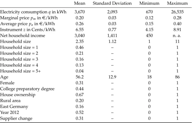
Before reporting billing information, the respondents were requested to gauge the marginal price per kWh they had to pay for 2012, yet without looking at their bills. By comparing each household’s estimate with the price that was actually paid, we have been able to construct an indicator for a household’s price knowledge: If a household’s ex-ante estimate deviates by less than±20% from the actual marginal price, this indi- cator takes on the value of 1 and 0 otherwise. According to this definition, 61% of our sample households have a coarse impression of electricity prices (Table 1). Alternative bandwidths using deviations of ± 10% and ± 15% have also been employed for the definition of price knowledge, leaving our estimation results largely unaltered.
Identification of the switching regression model, described in detail in Section 5, requires at least one variable that determines the respondents’ price knowledge, yet not their electricity consumption level. Such a variable would fulfill what is commonly called the exclusion restriction. To this end, we exploit the information on whether a household changed its electricity supplier during the three years prior to the survey (Supplier Change = 1). It seems plausible that households searching for a new supplier might gather information on tariffs and prices and, hence, become familiar with power prices.
It bears noting that with 3,670 kWh, our sample households’ average electricity consumption per annum roughly matches the annual consumption of a typical Ger- man household, which amounts to about 3,500 kWh according to BNetzA (2014). Fur- thermore, the average price of 26 cents per kWh obtained from our sample fits to the mean household price of 25.89 cents that is published by Eurostat (2015) for 2012. The difference between the means of the average and marginal prices of 6 cents (Table 1) indicates that the fixed fee accounts for around one quarter of total electricity costs.
Withe3,041 per month, the mean net income of our sample households is very close to the e 3,069 that is reported as average income for German households in 2012 by the German Federal Statistical Office (Destatis, 2015).
Unlike electricity consumption, prices, and net income, there are substantial diffrences
between our sample and the German population with respect to other variables. For example, with 67%, the share of home owners in our sample is far higher than the share of 45.9% that is published by the German Federal Statistical Office (Destatis, 2014b). A key reason for this discrepancy is that in responding to the survey questions on electric- ity cost and consumption for 2012, the share of tenants who can resort to information from electricity bills is lower than the respective share of home owners, not least due to the fact that tenants move more frequently than home owners. Not surprisingly, as it was the household heads and, hence, exclusively adult household members who were asked to respond to our survey, the respondents’ mean age of 56.2 years is higher than the average of 45.9 years for the German population (Destatis, 2014a).
Table 1:Descriptive Statistics for the Estimation Sample
Mean Standard Deviation Minimum Maximum
Electricity consumptionqin kWh 3,670 2,093 670 26,535
Marginal pricepmine/kWh 0.20 0.03 0.12 0.28
Average price paine/kWh 0.26 0.03 0.15 0.40
Instrumentzin Cents/kWh 6.55 0.77 4.15 8.91
Net household income 3,040 1,411 450 n. a.
Household size 2.35 1.12 1 11
Household size = 1 0.46 – 0 1
Household size = 2 0.21 – 0 1
Household size = 3 0.16 – 0 1
Household size = 4 0.13 – 0 1
Household size = 5+ 0.04 – 0 1
Age 56.2 12.9 18 86
Female 0.31 – 0 1
College preparatory degree 0.44 – 0 1
House ownership 0.67 – 0 1
Rural area 0.20 – 0 1
East Germany 0.16 – 0 1
Year 2012 0.52 – 0 1
Supplier change 0.31 – 0 1
As instrumentzfor the likely endogenous price variables, we employ the compos- ite of local grid and license fees, which are region-specific and account for about one quarter of the average consumer price (BDEW, 2016:48). Hence, our instrument z is correlated with the consumer price, but due to the exogeneity of grid and license fees to individual households, it seems to be warranted to assume that these price compo-
nents do not affect consumers’ tariff choice and consumption levelq. Hence, in formal terms, our instrumentzshould, apart from its correlation with consumer price p, nei- ther affect the consumption levelq, nor shouldzbe correlated with the error termεof any regression specification. In short, both identification assumptions for valid instru- ments should hold: (1)Cov(p,z)6=0 and (2)Cov(ε,z) =0.
While taxes and levies, such as the surcharge for the support of renewable tech- nologies, are the same for all household consumers, grid and license fees significantly differ across regions. In fact, grid fees are the highest in those federal states with the strongest expansion of wind power capacities, most notably in North and East Ger- many, as the connection of these additional capacities necessitates the augmentation and enhancement of the existing power grids, as well as the installation of new power lines.3
4 Panel Estimation Results
To contribute to the ongoing debate on the kind of price measure that is relevant for consumer decisions, we begin by including two alternative price measures in our es- timations, either the marginal or the average price. To provide for a reference case for our IV estimates, we use standard panel estimation methods and estimate a double-log specification, which is typically employed for estimating elasticities:
ln(qit) =α+αp·ln(pit) +αT·xit+γi+εit, (3)
where ln(qit) denotes the natural logarithm of the annual electricity consumption qit of householdiat timet, pstands for either the marginal or the average price, pm orpa, xis a vector of household characteristics, γidenotes the household-specific effect and εdesignates the error term.
3Data on grid and license fees at the postcode level for the years 2011 and 2012 were purchased from ene’t, a professional provider of energy-related data. If grid and license fees changed during a calendar year, we have taken the weighted mean of these fees, weighted by the days of their validity.
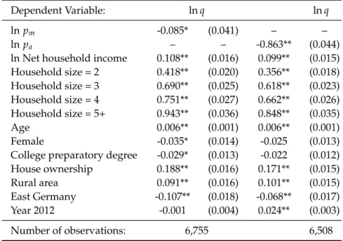
While we have deliberately refrained from reporting fixed-effects estimates due to the large number of time-persistent variables, our random-effects estimation results for structural Equation 3 indicate that both marginal and average prices have statistically significant effects on electricity demand (Table 2). With about -0.86, the demand elas- ticity with respect to average prices is considerably larger than that for marginal prices, which is quite close to, but in statistical terms different from zero. The estimate of -0.86 is in line with the results of Taylor et al. (2004), who demonstrate that estimations using average prices are biased towards -1. This casts doubt on the usage of average prices as the preferred price measure.
Table 2: Random-Effects Estimation Results for Logged Annual Electricity Con- sumption either with Marginal or Average Prices as Regressors
Dependent Variable: lnq lnq
lnpm -0.085* (0.041) – –
lnpa – – -0.863** (0.044)
ln Net household income 0.108** (0.016) 0.099** (0.015) Household size = 2 0.418** (0.020) 0.356** (0.018) Household size = 3 0.690** (0.025) 0.618** (0.023) Household size = 4 0.751** (0.027) 0.662** (0.026) Household size = 5+ 0.943** (0.036) 0.848** (0.035)
Age 0.006** (0.001) 0.006** (0.001)
Female -0.035* (0.014) -0.025 (0.013)
College preparatory degree -0.029* (0.013) -0.022 (0.012) House ownership 0.188** (0.016) 0.171** (0.015)
Rural area 0.091** (0.016) 0.101** (0.015)
East Germany -0.107** (0.018) -0.068** (0.017)
Year 2012 -0.001 (0.004) 0.024** (0.003)
Number of observations: 6,755 6,508
Note: Standard errors are in parentheses and clustered at the post code level; * and ** denote sta- tistical significance at the 5% and 1% level, respectively.
When employing marginal prices for estimating electricity demand responses, how- ever, one must be skeptical, as well. Since the liberalization of Germany’s electricity market in 1998, households are free to choose from a wide variety of providers and tariffs. Hence, marginal electricity prices are likely to be endogenous, as rational cus- tomers tend to select contracts that minimize their electricity costs. In contrast, in former monopolistic markets, households had no opportunity at all to choose their
provider and tariff, but were stuck with their local electricity provider, and, thus, elec- tricity prices were clearly exogenous.
Yet, the price structure of the former monopolistic era, including a monthly fixed fee, as well as a constant marginal price that is independent of consumption levels, still remains the dominant tariff today, whereas alternatives, such as package and flat- rate tariffs, are rarely offered. As changing both suppliers and tariffs have become a common phenomenon, a simultaneity problem may arise: while, on the one hand, consumption levels tend to be affected by prices, on the other hand, households’ tariff selection may depend on consumption levels.
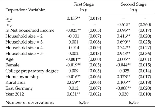
To cope with this simultaneity problem, we pursue a random-effects panel IV ap- proach and employ the composite of the local grid and license fees as instrumental variable z for the likely endogenous marginal price, noting that a correlation coeffi- cient of 0.23 indicates the expected positive correlation betweenzand marginal prices pm. This positive correlation can also be observed from the estimation results of the first stage of the IV regression that is given by Equation 4:
ln(pit) = β+βz·ln(zit) +βT·xit+νit, (4)
where the marginal pricepm is regressed on our instrumental variablezand the vector x of household characteristics, while νdesignates another error term. Given that the coefficient estimate on lnzreported in Table 3 is positive and statistically significant at the 1% significance level, there is statistical evidence that the first assumption for valid instruments holds: Cov(p,z) 6=0.
At the second stage of the IV approach, instead of employing observed prices pm, structural Equation 3 is estimated using the predictions ln[pm, which are obtained from estimating first-stage Equation 4. The results of the second-stage regression in- dicate that, approximately, a 10% increase in marginal electricity prices comes along with a decrease in electricity use of -6.2%. Using cross-sectional data originating from
Germany’s Income and Expenditure Survey, which is conducted at 5-year intervals, Schulte and Heindl (2016) find a quite similar own-price elasticity of 0.43 for residen- tial electricity consumption (1993-2008).
Much less elastic is the household response with respect to income: An increase in household net income by 10% induces an increase in electricity consumption of about 1%. The outcomes of the remaining variables are largely in accord with our expecta- tions: Whileceteris paribus home owners, older people, and those living in rural areas have a higher electricity consumption than other households, it is a well-known fact that, on average, households residing in East Germany consume less electricity (RWI and forsa, 2016), as well as households with a female head. Not surprisingly, house- hold size is an important driver of electricity consumption. The electricty use of a 3- person household, for example, is 100[exp(0.69)-1]=99% higher than that of a 1-person household.
Table 3: Random-Effects Panel Instrumental-Variable (IV) Results for Logged An- nual Consumption
First Stage Second Stage
Dependent Variable: lnp lnq
lnz 0.155** (0.018) – –
lndp – – -0.615* (0.260)
ln Net household income -0.023** (0.005) 0.096** (0.017) Household size = 2 -0.001 (0.007) 0.416** (0.020) Household size = 3 0.001 (0.008) 0.690** (0.025) Household size = 4 -0.014 (0.009) 0.742** (0.027) Household size = 5+ 0.002 (0.013) 0.943** (0.036)
Age -0.001** (0.000) 0.005** (0.001)
Female -0.019** (0.005) -0.044** (0.015)
College preparatory degree 0.009 (0.005) -0.025 (0.014)
Home ownership -0.016** (0.006) 0.178** (0.017)
Rural area 0.029** (0.006) 0.105** (0.018)
East Germany 0.012 (0.007) -0.088** (0.020)
Year 2012 0.031** (0.002) 0.020 (0.010)
Number of observations: 6,755 6,755
Note: Standard errors are in parentheses and clustered at the post code level; * and ** denote statistical significance at the 5% and 1% level, respectively.
An important drawback of IV estimates is that their standard errors are typically
larger than those of the respective OLS estimates (Bauer et al., 2009:327). In fact, if a variable that is deemed to be endogenous is instead exogenous, the IV estimator will be less efficient than the OLS estimator, while both estimators will be consistent.
If an instrument is only weakly correlated with an endogenous regressor, the loss of precision of IV estimators may be severe. Even worse is that with weak instruments, IV estimates are inconsistent and biased in the same direction as OLS estimates (Chao and Swanson, 2005). Most disconcertingly, as is pointed out by Bound et al. (1993, 1995), when the instruments are only weakly correlated with the endogenous variables, the cure in the form of the IV approach can be worse than the disease resulting from biased and inconsistent OLS estimates. Given these potential problems, it is reasonable to perform an endogeneity test that examines whether a potentially endogenous variable is in fact exogenous.
To this end, following the essential idea of the Durbin-Wu-Hausman test for endo- geneity (Hausman, 1978), we test whether the error termνof Equation 4 is correlated with the error term ε of structural Equation 3. Although neither ε nor ν can be ob- served, one can employ the residuals of the first- and second-stage regressions and test whether they are correlated. Alternatively, one can plug the residual ˆνas an additional regressor into structural Equation 3 and test its statistical significance (Davidson and MacKinnon, 1989). As a result, we get a coefficient estimate – not reported here – that is significant at the one percent level, providing strong evidence for the endogeneity of marginal prices.
While this outcome suggests the application of the IV approach, its validity de- pends on the strength of our instrument. Given that the standard errors are not iden- tically distributed, nor independent, as observations are clustered at the household level, the weakness of instruments is tested using a Wald test (Kleibergen and Paap, 2006). With an F statistic of F = 116.1 for the coefficient βz of the first-stage regression 4, which is well above the threshold of 16.38 given by Stock and Yogo (2005), we can reject the null hypothesis of weak identification.
5 The Effect of Price Knowledge
In this section, we exploit the information on the households’ knowledge about power prices by employing an Endogenous Switching Regression Model (Maddala, 1983) to estimate price responses for two groups of households, those that are informed about current price levels (Group 1) and those that are unaware of prices (Group 0):
price knowledge=
1 ifγ·wi ≥ui, 0 otherwise,
(5)
In this definition, wi denotes those household characteristics that may affect whether a household is informed about prices (Group 1: price knowledge = 1), γ is the corre- sponding parameter vector, and the error termuis assumed to be correlated with both error terms η1 andη0emerging from the following structural equations, as there may be unobservable factors that are relevant for both the selection into either group and the consumption level.
In line with structural Equation 3, the behavioral response of households due to price changes is described by two equations:
ln(q1it) = α1+α1p·ln(pit) +α1·x1it−σ1u·IVM1i+η1itif price knowledge = 1, (6) ln(q0it) = α0+α0p·ln(pit) +α0·x0it+σ0u·IVM0i+η0itif price knowledge = 0, (7)
whereη1andη0are error terms with zero conditional mean and
IVM1i := φ(γT ·zi)
Φ(γT·zi), IVM0i := φ(γT ·zi)
1−Φ(γT·zi) (8) represent the two variants of the inverse Mills ratios, with φ(.)and Φ(.)denoting the density and cumulative density function of the standard normal distribution, respec- tively. When appended as extra regressors in the second-stage estimation, the inverse Mills ratios are controls for potential biases arising from sample selectivity. Selectiv-
ity is likely, as unobservable characteristics, such as carelessness about electricity con- sumption and bills, may affect both consumption levels and price awareness. If the estimated coefficients –σ1uandσ0u – are statistically significant, this is an indication of sample selectivity.
To investigate this issue, for the second-stage regression, we insert the predicted values[IVM1iand [IVM0i, as well as the predictions for the endogenous marginal price variable, using the probit estimatesγbof the first-stage estimation (Andor et al., 2016).
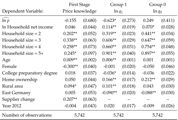
Alternatively, we have also estimated the above switching regression model for the pooled sample using the full information maximum likelihood (FIML) estimator, as it is more efficient than two-stage least squares methods and the maximum likelihood estimator and provides consistent standard errors (Lokshin and Sajaia, 2004). To this end, we have employed the Stata command movestay (Lokshin and Sajaia, 2004). The results, reported in Table A.1 of the appendix, are similar – in qualitative terms – to those displayed in Table 4.
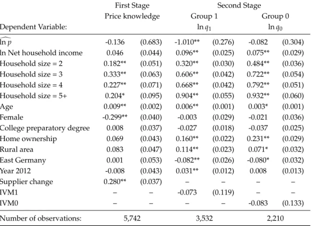
The probit estimation results for the first stage of the switching regression model, reported in the first column of Table 4, indicate that whether a household changed its electricity provider during the three years prior to the interview positively affects its price knowledge: The probability that such households are informed about price levels increases by 28 percentage points relative to those that did not change their supplier.
To check whether selection bias is an issue and, hence, whether the use of a switch- ing regression model is appropriate, we have performed a Wald test on the indepen- dence of Equations 6 and 7. The test statistic – not reported here – indicates that the null hypothesis of independent equations can be rejected at the 1% significance level.
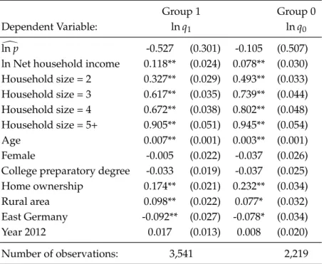
Note, however, that both coefficient estimates on the inverse mills ratios are not sta- tistically significant and, in qualitative terms, the estimation results displayed in Table 4 are similar to the random-effects IV estimates for the split sample (see Table A.2 in the appendix), where structural Equation 3 is estimated separately for each subsample, Group 0 and Group 1, without any control for selection bias.
Table 4: Random-Effects Two-Step Switching Regression Results
First Stage Second Stage
Price knowledge Group 1 Group 0
Dependent Variable: lnq1 lnq0
lndp -0.136 (0.683) -1.010** (0.276) -0.082 (0.304)
ln Net household income 0.046 (0.044) 0.096** (0.025) 0.075** (0.029) Household size = 2 0.182** (0.051) 0.320** (0.030) 0.484** (0.036) Household size = 3 0.333** (0.063) 0.606** (0.042) 0.722** (0.054) Household size = 4 0.227** (0.071) 0.668** (0.042) 0.792** (0.051) Household size = 5+ 0.204* (0.095) 0.904** (0.055) 0.932** (0.060)
Age 0.009** (0.002) 0.006** (0.001) 0.003* (0.001)
Female -0.299** (0.040) -0.003 (0.029) -0.021 (0.036)
College preparatory degree 0.008 (0.037) -0.027 (0.018) -0.037 (0.025) Home ownership 0.069 (0.043) 0.160** (0.022) 0.231** (0.029)
Rural area 0.083 (0.047) 0.114** (0.023) 0.071* (0.032)
East Germany 0.001 (0.053) -0.082** (0.026) -0.080* (0.032)
Year 2012 -0.008 (0.043) 0.031** (0.012) 0.008 (0.013)
Supplier change 0.280** (0.037) – – – –
IVM1 – – -0.073 (0.119) – –
IVM0 – – – – -0.083 (0.133)
Number of observations: 5,742 3,532 2,210
Note: Standard errors are in parentheses and clustered at the post code level; * and ** denote statistical significance at the 5%
and 1% level, respectively.
In sum, sample selection issues notwithstanding, in line with the literature (see e. g. Gaudin (2006) and Carter and Milon (2005)), we find evidence that households with a crude idea about current price levels (Group 1) are more price-elastic than un- informed households (Group 0). In fact, for price-ignorant households, the price elas- ticity estimate does not differ from zero at any conventional significance level (Table 4).
6 Summary and Conclusions
Consistently estimating consumer demand responses is frequently hampered by the prevalence of tariffs that include a fixed fee. Such tariffs are standard in numerous retail markets, such as telecommunication and electricity markets. The endogeneity
problem arising from such a tariff structure is aggravated when consumers are free to choose from a broad range of tariffs, as is common in Germany since the liberalization of European electricity markets in 1998. To cope with the endogeneity resulting from tariff choice, we have employed an instrumental-variable (IV) approach, using panel data from the German Residential Energy Consumption Survey (GRECS) for the years 2011 and 2012. The IV estimate of the price elasticity of electricity demand of about -0.62 indicates that, on average, households respond to power price changes.
This general conclusion, however, does not hold unequivocally: By additionally exploiting our information on the households’ knowledge about power prices and em- ploying an instrumental-variable Endogenous Switching Regression Model in which we have replaced the endogenous marginal price variable by the predicted prices orig- inating from the first-stage regression, we come up with the more differential con- clusion that price knowledge appears to be crucial for demand response. In line with Wolak (2011) and Jessoe and Rapson (2014), who find that information provision changes the price elasticity of electricity demand, our results indicate that only those house- holds that are informed about prices are sensitive to price changes, whereas the elec- tricity demand of uninformed households is entirely price-inelastic.
With respect to the external effects of electricity generation, our findings suggest that further increases in power prices, which are a likely consequence of Germany’s ambitious transition of its energy system, only leads to substantial demand reductions and corresponding environmental benefits if households are aware of marginal prices.
In addition to non-price interventions, such as social norm comparisons, which have proved to be cost-effective in the U. S. (Allcott, 2011), we therefore propose fostering information measures to improve the price awareness of households, not least because providing price information has the potential to improve market efficiency. This is all the more relevant, as due to recent technological developments, a growing number of consumers can get access to real-time feedback on their price and consumption data (Ito, 2014:561).
Appendix
Table A.1: FIML Switching Regression Estimations Results
First Stage Group 1 Group 0
Dependent Variable: Price knowledge lnq1 lnq0
lndp -0.155 (0.680) -0.623* (0.273) 0.249 (0.411)
ln Household net income 0.046 (0.044) 0.114** (0.019) 0.070* (0.028) Household size = 2 0.202** (0.052) 0.319** (0.023) 0.441** (0.034) Household size = 3 0.338** (0.063) 0.606** (0.029) 0.647** (0.059) Household size = 4 0.258** (0.073) 0.660** (0.031) 0.754** (0.048) Household size = 5+ 0.245* (0.097) 0.901** (0.040) 0.897** (0.055)
Age 0.009** (0.002) 0.006** (0.001) 0.001 (0.001)
Female -0.300** (0.040) -0.001 (0.020) -0.050 (0.046)
College preparatory degree 0.018 (0.037) -0.036* (0.014) -0.036 (0.022) Home ownership 0.050 (0.044) 0.166** (0.017) 0.212** (0.029) Rural area 0.094* (0.047) 0.101** (0.018) 0.043 (0.030) East Germany 0.005 (0.053) -0.090** (0.020) -0.088** (0.030)
Supplier change 0.207** (0.063) – – – –
Year 2012 -0.004 (0.043) 0.020 (0.017) -0.009 (0.026)
Number of observations: 5,742 5,742 5,742
Note: Standard errors are in parentheses and clustered at the post code level; * and ** denote statistical significance at the 5% and 1% level, respectively.
Table A.2: Split Sample Random-Effects IV Estimation
Group 1 Group 0
Dependent Variable: lnq1 lnq0
lndp -0.527 (0.301) -0.105 (0.507)
ln Net household income 0.118** (0.024) 0.078** (0.030) Household size = 2 0.327** (0.029) 0.493** (0.033) Household size = 3 0.617** (0.035) 0.739** (0.044) Household size = 4 0.672** (0.038) 0.802** (0.048) Household size = 5+ 0.905** (0.051) 0.945** (0.054)
Age 0.007** (0.001) 0.003** (0.001)
Female -0.005 (0.022) -0.037 (0.026)
College preparatory degree -0.033 (0.019) -0.037 (0.025) Home ownership 0.174** (0.021) 0.232** (0.034) Rural area 0.098** (0.022) 0.077* (0.032) East Germany -0.092** (0.027) -0.078* (0.034)
Year 2012 0.017 (0.013) 0.008 (0.020)
Number of observations: 3,541 2,219
Note: Standard errors are in parentheses and clustered at the post code level; * and ** denote statistical significance at the 5% and 1% level, respectively.
References
Allcott, H., 2011. Social Norms and Energy Conservation. Journal of Public Economics 95 (9-10), 1082–1095.
Andor, M., Frondel, M., Vance, C., 2016. Mitigating Hypothetical Bias: Evidence on the Efforts of Correctives from a Large Field Study.Environmental and Resource Economics.
Baker, P., Blundell, R., Micklewright, J., 1989. Modelling Household Energy Expendi- tures Using Micro-Data.The Economic Journal99 (397), 720–738.
Bauer, T. K., Fertig, M., Schmidt, C. M., 2009. Empirische Wirtschaftsforschung, Eine Einführung. Springer, Berlin Heidelberg.
BDEW, 2016. Erneuerbare Energien und das EEG: Zahlen, Fakten, Grafiken. Bun- desverband der Energie- und Wasserwirtschaft, Berlin, 18. Februar 2016.
BNetzA, 2014. Monitoringbericht 2014. Bundesnetzagentur, Bonn.
Borenstein, S., 2009. To What Electricity Price do Consumers Respond? Residential Demand Elasticity Under Increasing-Block Pricing. Preliminary draft, University of California.
Bound, J., Jaeger, D. A., Baker, R., 1993. The Cure Can be Worse Than the Disease: A Cautionary Tale Regarding Instrumental Variables. Working paper, National Bureau of Economic Research, Cambridge, Massachusetts.
Bound, J., Jaeger, D. A., Baker, R. M., 1995. Problems With Instrumental Variables Es- timation When the Correlation Between the Instruments and the Endogenous Ex- planatory Variable is Weak. Journal of the American Statistical Association 90 (430), 443–450.
Carter, D. W., Milon, J. W., 2005. Price Knowledge in Household Demand for Utility Services.Land Economics81 (2), 265–283.
Chao, J. C., Swanson, N. R., 2005. Consistent Estimation With a Large Number of Weak Instruments.Econometrica73 (5), 1673–1692.
Davidson, R., MacKinnon, J. G., 1989. Testing for Consistency Using Artificial Regres- sions.Econometric Theory5 (3), 363–384.
Destatis, 2014a. Durchschnittsalter in den Bundesländern.
URL www.destatis.de/DE/ZahlenFakten/GesellschaftStaat/Bevoelkerung/
Bevoelkerungsstand/Bevoelkerungsstand.html;16.03.2015
Destatis, 2014b. Eigentümerquote 2011.
URL www.destatis.de/DE/ZahlenFakten/GesellschaftStaat/
EinkommenKonsumLebensbedingungen/Wohnen/Wohnen.html;16.03.2015
Destatis, 2015. Einkommen, Einnahmen und Ausgaben privater Haushalte im Zeitver- gleich.
URL www.destatis.de/DE/ZahlenFakten/GesellschaftStaat/
EinkommenKonsumLebensbedingungen/EinkommenEinnahmenAusgaben/Tabellen/
Deutschland.html;16.03.2015
Espey, J. A., Espey, M., et al., 2004. Turning on the Lights: a Meta-Analysis of Resi- dential Electricity Demand Elasticities.Journal of Agricultural and Applied Economics 36 (1), 65–82.
Eurostat, 2015. Energy, Transport and Environment Indicators, 2015 Edition. European Commission, Luxemburg.
Fell, H., Li, S., Paul, A., 2014. A New Look at Residential Electricity Demand Using Household Expenditure Data.International Journal of Industrial Organization 33, 37–
47.
Frondel, M., Sommer, S., Vance, C., 2015. The Burden of Germany’s Energy Transition:
An Empirical Analysis of Distributional Effects.Economic Analysis and Policy45, 89–
99.
Gaudin, S., 2006. Effect of Price Information on Residential Water Demand. Applied Economics38 (4), 383–393.
Hausman, J. A., 1978. Specification Tests in Econometrics. Econometrica 46 (6), 1251–
1271.
Ito, K., 2014. Do consumers respond to marginal or average price? Evidence from nonlinear electricity pricing.The American Economic Review104 (2), 537–563.
Jessoe, K., Rapson, D., 2014. Knowledge is (less) Power: Experimental Evidence from Residential Energy Use.The American Economic Review104 (4), 1417–1438.
Kleibergen, F., Paap, R., 2006. Generalized Reduced Rank Tests Using the Singular Value Decomposition.Journal of Econometrics133 (1), 97–126.
Lokshin, M., Sajaia, Z., 2004. Maximum Likelihood Estimation of Endogenous Switch- ing Regression Models.Stata Journal4, 282–289.
Maddala, G. S., 1983. Limited-Dependent and Qualitative Variables in Econometrics.
Cambridge University Press.
Reiss, P. C., White, M. W., 2005. Household Electricity Demand, Revisited.The Review of Economic Studies72 (3), 853–883.
RWI, forsa, 2016. Erhebung des Energieverbrauchs der privaten Haushalte.
URLwww.rwi-essen.de/haushaltsenergieverbrauch;13.10.2016
Schulte, I., Heindl, P., 2016. Price and Income Elasticities of Residential Energy Demand in Germany. Zew discussion paper no. 16-052, Center for Eureopean Economic Re- seach, Mannheim, Germany.
Shin, J.-S., 1985. Perception of Price when Price Information is Costly: Evidence from Residential Electricity Demand.The Review of Economics and Statistics67 (4), 591–598.
Stock, J. H., Yogo, M., 2005. Testing for Weak Instruments in Linear IV Regression.
Identification and Inference for Econometric Models: Essays in Honor of Thomas Rothenberg.
Taylor, L. D., 1975. The Demand for Electricity: a Survey.The Bell Journal of Economics 6 (1), 74–110.
Taylor, R. G., McKean, J. R., Young, R. A., 2004. Alternate Price Specifications for Esti- mating Residential Water Demand With Fixed Fees.Land Economics80 (3), 463–475.
Wolak, F. A., 2011. Do Residential Customers Respond to Hourly Prices? Evidence From a Dynamic Pricing Experiment.The American Economic Review101 (3), 83–87.