Switching to green electricity: Spillover effects on household consumption

(1)

SFB 823

Switching to green electricity:

Spillover effects on household consumption

Discussion Paper Stephan Sommer

Nr. 24/2018

(2)

(3)

Switching to Green Electricity: Spillover Effects on Household Consumption

Stephan Sommer

^*

October 13, 2018

One way to reduce emissions from the consumption of electricity is switching to green electricity suppliers. This paper identifies the determinants of adopting green electricity and the effect on electricity consumption, using panel data on more than 9,000 households. To control for potential self-selection into green electricity tariffs, an endogenous dummy treatment effects model is estimated. The results suggest that wealthier and better-educated households are more likely to adopt green electricity. Moreover, we find that switching to green electricity decreases electricity consumption and households supplied by green electricity are less price-responsive. Consequently, enforcing higher prices for conventional electricity might prove effective in reducing both greenhouse gas emissions and electricity consumption at the household level.

JEL Codes:D12, H31, H41, Q41.

Keywords:Electricity demand, Endogenous treatment, Difference-in-differences, Price elasticity.

Acknowledgements: Special thanks go to Manuel Frondel for invaluable feedback and dis- cussions. Moreover, I thank Fabian Feger, Andreas Gerster, Vera Huwe, Gerhard Kussel, Francesca Paolini, and participants of the 23rd Annual Conference of Environmental &

Resource Economics in Athens for very helpful comments. Furthermore, I gratefully ac- knowledge financial support by the Federal Ministry of Education and Research (BMBF) under grant 01UT1701A (LICENSE). This work has also been supported by the Collabora- tive Research Center “Statistical Modeling of Nonlinear Dynamic Processes” (SFB 823) of the German Research Foundation (DFG), within Project A3, Dynamic Technology Mod- eling.

*RWI Leibniz Institute for Economic Research. Hohenzollernstraße 1-3, D-45128 Essen. Email:

sommer@rwi-essen.de.

(4)

1 Introduction

Reducing and internalizing the external effects of greenhouse gas emissions is a ma- jor goal of environmental economics. Besides traditional policy instruments to reduce emissions, such as command-and-control measures and taxes (Dietz et al., 2003), consumers of electricity might voluntarily avoid negative externalities that emerge from the conventional production of electricity by switching to suppliers with a portfolio of renewable energy sources. Although most households prefer renewable-based over fossil-fuel- based electricity and are even willing to pay a notable mark-up (Andor et al., 2017; Sundt and Rehdanz, 2015), only a small percentage of customers is supplied by green electricity. Among the barriers to the adoption of green electricity are perceived higher financial costs, limited knowledge, the awareness of green tariffs (Hobman and Frederiks, 2014;

He and Reiner, 2017), as well as conventional default options (Ebeling and Lotz, 2015;

Sunstein and Reisch, 2014) and consumer inertia (Hortaçsu et al., 2017).

Using panel data on about 9,000 German households that reported comprehensive billing data and socioeconomic characteristics, this paper identifies the determinants of adopting green electricity and the spillover effect on household electricity consumption for the period between 2011 and 2016. Furthermore, we quantify the price elasticity of demand, as potential changes in consumption patterns might be caused by higher prices.

Since the decision to adopt green electricity and the consumption level may be interre- lated, we are faced with potential self-selection problems. To address this issue, an endogenous dummy treatment effects model (Heckman, 1976, 1978) is estimated, using the number of nearby windmills and the distance to the next nuclear power plant as instruments.

Abstracting from price effects, households may either decrease or increase their electricity consumption after subscribing to green electricity, exhibiting positive or neg-

(5)

ative spillovers, respectively (e.g. Dolan and Galizzi, 2015 and Truelove et al., 2014 for overviews of spillover effects). If the adoption of one moral behavior (switching to green electricity) increases the household’s inclination to engage in another moral behavior (reduce electricity consumption), it exhibits positive spillovers, which are caused by the desire to behave consistently (Thøgersen and Crompton, 2009). In contrast, switching to green electricity may liberate households to engage in an immoral, unethical or otherwise problematic behavior (Merritt et al., 2010), resulting in higher electricity consumption levels. This negative spillover effect is referred to as moral licensing (e.g. Blanken et al., 2015 and Miller and Effron, 2010).¹

Thus far, empirical studies on spillover effects of adopting green electricity are scarce and have primarily been conducted in the US, where households consume notably more electricity than in Germany and most other European countries (WEC, 2017) and differ in environmental attitudes (e.g. Olofsson and Öhman, 2006; PEW, 2015). For instance, Hard- ing and Rapson (2017) observe that after enrolling in an electricity program that offsets customers’ carbon emissions, some households – especially young and wealthy households – increase their consumption. Although Jacobsen et al. (2012) do not detect an overall effect on electricity consumption for households that participate in a green electricity program, they find that households that purchase the smallest possible amount of green electricity subsequently increase their consumption by 2.5%, a behavior they refer to as buy-in mentality. In contrast, Kotchen and Moore (2008) observe that households that do not care about the externalities of their electricity consumption (so-called non-conservationists) reduce it after participating in a green electricity program, whereas conservationists do not exhibit any change. They trace this behavior back to the price premium for green tariffs.

1The moral licensing effect can also occur across domains. For instance, in a field experiment, Tiefen- beck et al. (2013) show that households who received weekly feedback on their water consumption lowered water usage, but increased their electricity consumption at the same time.

(6)

In line with the literature (Conte and Jacobsen, 2016; Clark et al., 2003; Kotchen and Moore, 2007), we find that the average subscriber to green electricity is environmentally more concerned, wealthier, and better educated than customers of conventional electricity. This has important implications for the marketing of green electricity programs. Par- ticipation rates in of green electricity programs can be increased if they are targeted at households that are most likely to adopt green electricity (Kotchen and Moore, 2007).

This targeted marketing can also reduce marketing expenditures, resulting in a more cost-effective use of resources (Conte and Jacobsen, 2016). Moreover, our results suggest that households – particularly conservationists – lower their electricity consumption after adopting green electricity. As this effect is substantially larger than the estimated price elasticity would imply, households seem to lower electricity consumption for other reasons, reflecting a positive spillover effect. Given that households with green tariffs voluntarily curb emissions from and households with conventional tariffs exhibit stronger price reactions, pecuniary instruments on conventional electricity may prove effective in further reducing electricity consumption and related greenhouse gas emissions.

2 Data

Our analysis relies on comprehensive household panel data, originating from the German Residential Energy Consumption Survey (GRECS). The data was gathered in co- operation with the professional survey instituteforsa, usingforsa’s household panel that is representative for the German population aged 14 and above (RWI and forsa, 2015).² In four panel waves, participants reported socioeconomic as well as detailed billing information for the period between 2011 and 2016. Data was collected byforsavia a state-of- the-art tool that allows respondents to complete the questionnaire at home using either

2For more information onforsaand its household panel, see http://www.forsa.com.

(7)

the internet or a television. Respondents could interrupt and continue the questionnaire at any time. The participating households were asked to provide electricity cost and consumption figures from their latest electricity bills covering the preceding years. If several bills exist for one specific year, we combined the billing data to compute annual total expenditures and consumption figures. Dividing annual total expenditures by consumption yields average electricity prices, which will be used in the upcoming analysis.³

We only use electricity bills with a duration of more than 180 days to exclude sea- sonal impacts. Owing to possible typing errors, we clean the data set via an iterative process that drops observations whose consumption figure and average price do not lie within an interval that spans two standard deviations around the mean, separated by household size. In addition, households that solely heat with electricity are excluded because in contrast to other countries such as the US, electric heating is not very common in Germany and only used among 3% of the households (RWI and forsa, 2015). Overall, we retrieve 15,573 observations with information on electricity consumption, electricity prices, and the source of the electricity (green or conventional) from 9,009 households.

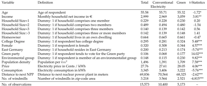
For all sample households, we observe a large suite of socioeconomic characteristics and merge it with regional data (Table 1). On average, our respondents are 56 years old.

Household net monthly income is measured in intervals ofe500 and top-coded ate5,700.

For our purposes, we assign the middle value of the indicated interval to each household and observe a mean income of about e3,000. Around 23% of the respondents live in a single household, while 28% live in households with three or more members, indicating the existence of children. About two thirds of the respondents live in their own dwelling and some 30% of the respondents hold a college degree. With a share of 32% women are considerably less frequent in the sample than men. This circumstance can be traced back

3In the literature, there is a discussion about whether households respond to average or (expected) marginal prices. Although economic theory suggests that people react to marginal prices, empirical evidence reveals that they rather react to average prices because of limited attention to complex pricing sched- ules (Borenstein, 2009; Ito, 2014).

(8)

to our decision to ask only household heads to participate in the survey, as by definition, they typically make financial decisions at the household level, including the choice of the electricity supplier. Table A1 in the Appendix shows that for many characteristics our sample closely matches the population of German household heads, while for instance, elderly individuals and homeowners are overrepresented.

Table 1:Summary Statistics

Variable Definition Total Conventional Green t-Statistics

Electricity

Age Age of respondent 55.58 55.71 55.32 -1.72*

Income Monthly household net income ine 2,999 2,969 3,059 3.81**

Household Size=1 Dummy: 1 if household comprises one member 0.229 0.228 0.230 0.20 Household Size=2 Dummy: 1 if household comprises two members 0.489 0.494 0.480 -1.54 Household Size=3 Dummy: 1 if household comprises three members 0.140 0.139 0.142 0.56 Household Size>3 Dummy: 1 if household comprises three or more members 0.142 0.139 0.148 1.41

Homeowner Dummy: 1 if household lives in an own dwelling 0.664 0.665 0.661 -0.47

College Degree Dummy: 1 if respondent has college degree 0.295 0.281 0.324 5.48***

Female Dummy: 1 if respondent is female 0.320 0.308 0.344 4.57***

East Germany Dummy: 1 if household resides in East Germany 0.200 0.213 0.174 -5.74***

Green party Dummy: 1 if respondent tends to vote for the Green party 0.106 0.068 0.177 14.02***

Environmental group Dummy: 1 if respondent is member of an environmentalist group 0.148 0.115 0.230 9.82***

Population density Population perkm² 1,496 1,391 1,709 7.58***

Price Electricity price in Cents / kWh 27.76 27.61 28.05 4.06***

Consumption Electricity consumption in kWh 3,345 3,406 3,222 -5.76***

Distance to next NPP Distance to next nuclear power plant in meters 69,836 70,564 68,325 -2.62***

No. of windmills Number of windmills in zip-code area 3.218 3.564 2.521 -4.815***

No. of observations 15,573 10,400 5,173 –

Note:^∗∗∗,^∗∗, and^∗denote statistical significant mean differences between households that are supplied by green electricity and those that are supplied by conventional electricity at the 1 %, 5 %, and 10 % level, respectively.

While the first panel wave was merely focused on the elicitation of final residential energy consumption (RWI and forsa, 2015), in the remaining three panel waves, we included additional questions on the socioeconomic background of the respondents. Of particular interest is whether households are members of an environmental group, which is the case for about 15% of the responding households. According to Kotchen and Moore (2008), this is an important determinant to classify households as either conservationists, i.e. households that care about the externalities of their electricity consumption, or non- conservationists because the latter group is found to be more likely to reduce electricity consumption after signing up for green electricity. Building upon Kotchen and Moore (2008), we characterize conservationists as members of an environmental group or voters

(9)

of the green party.

In general, since the liberalization of the German electricity market in 1998, households can freely choose their electricity supplier. Nevertheless, a vast majority of households stick with their default provider, although nowadays they can choose among almost 900 suppliers (BNetzA, 2018). About 20% of German residential customers are supplied by green electricity (UBA, 2015, p. 42). As the share of households with green electricity tariffs is about one third, they are overrepresented in our sample.

Unsurprisingly, the share of environmentally active households is significantly higher among adopters of green tariffs, as suggested by the mean comparison test result in the last column of Table 1. Furthermore, households are more likely to subscribe to green electricity if it is wealthy, resides in West Germany, and its head is female and a college graduate. The subscription to green electricity is also higher in more densely populated areas. Moreover, households supplied by green electricity consume significantly less electricity and pay higher prices per kilowatthour (kWh), resulting in lower total costs. De- spite higher prices, on average, green electricity households pay aboute37 less per year.

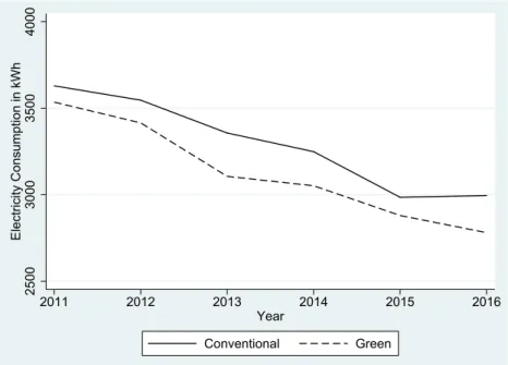
Figures 1 and 2 contrast mean electricity consumption and prices of customers of conventional and green electricity. The consumption of both conventional and green electricity declines notably over time, but throughout the sample period, customers of green electricity consume less. In contrast, electricity prices increase over time and on average households with green tariffs pay slightly more.

3 Methodological Issues

As households’ decision to adopt green electricity might be endogenous and, in for- mal terms, households can sort themselves into the treatment, simply regressing electric-

(10)

Figure 1:Mean Annual Electricity Consumption in kWh for Subscribers to Conventional and Green Electricity

2500300035004000Electricity Consumption in kWh

2011 2012 2013 2014 2015 2016

Year

Conventional Green

Figure 2: Mean Electricity Prices in ct/ kWh for Subscribers to Conventional and Green Electricity

2527293133Electricity Price in Cent / kWh

2011 2012 2013 2014 2015 2016

Year

Conventional Green

ity consumption on either type of electricity does not allow us to interpret the results in a causal way (Harding and Rapson, 2017). Unobservable household characteristics, such as environmental attitudes, may affect both the subscription to green electricity (Green) and

(11)

the amount of electricity consumed (y). Only if y were to be independent of Green, i.e.

only in case of random treatment assignment and in absence of self-selection, we could consistently determine the average treatment effect (ATE) as

AT E =E(y_it|x_it, Green_it = 1)−E(y_it|x_it, Green_it= 0). (1)

3.1 Two-Stage Dummy Endogenous Variable Model

To correct for self-selection, we apply the two-stage dummy endogenous variable model (Heckman, 1976, 1978), for the moment neglecting the panel character of our data set, but accounting for repeated observations by clustering standard errors at the household level. In our empirical example, treatment assignment is modeled by

Greenit=











1ifw⁰_itγ_w+u_it>0, 0otherwise

(2)

and the consumption equation is specified by

y_it=x⁰_itβ_x+δGreen_it+η_t+_it, (3)

where vector x comprises a set of socio-economic characteristics that are used to model electricity consumption y_it of householdi in yeart, vector wencompasses those covariates that affect whether a household switches to green electricity, and β_x andγ_w are the corresponding parameter vectors. Parameter δ represents the effect of adopting green electricity on electricity consumptionyandηcaptures year-fixed effects. The error terms uandare assumed to have a bivariate normal distribution with correlationρ.

If Equation (2) is estimated by a nonlinear function, vectorwcan contain the same

(12)

variables as vectorxto ensure the identification of the model (Maddala, 1983, p. 271). Yet, for a more robust identification, it is recommended to impose exclusion restrictions, i.e.

using at least one variable that determines the adoption of green electricity, but does not affect electricity consumption. If both assumptions hold, this variable can be interpreted as an instrumental variable (Angrist et al., 1996).

As instruments (z), the number of windmills at the zip code level and the distance to the next nuclear power plant are employed. The reasoning behind the choice of these variables is that after the incident in Fukushima in 2011, the German government boosted the deployment of renewable energy sources and stipulated the nuclear phase-out, which raised the consciousness of green electricity among households. We assume that z is uncorrelated to both disturbances and thus any effect ofzon electricity consumptionyis captured throughGreen. Furthermore, we assume thatcov(Green,z)6= 0.

The first stage of the dummy endogenous variable model involves estimating a probit model on the binary selection into treatment P(Greenit = 1|xit,zit) = G(xit,zit) con- ditional on a set of socio-economic characteristics (x) and instrumental variables (z). In a second step, the fitted probabilities Gb are used to estimate Equation (3) (Wooldridge, 2010).⁴ The consistent ATE is given by:

E(y_it|Green_it = 1,x_it,z_it)−E(y_it|Green_it = 0,x_it,z_it) (4)

=δ+ρσ

φ(w⁰_itγ)

Φ(w⁰_itγ)(1−Φ(w⁰_itγ))

,

whereρσ =cov(u, )andφ(.)andΦ(.)denote the standard normal density and distribution function, respectively. Neglecting self-selection issues and estimating Equation (3) using OLS would result in a biased coefficient. Sinceσ and the fraction in Equation (4) are positive, the direction of the bias hinges on the sign ofρ(Greene, 2003, p. 890).

4To estimate this model, we invoke Stata’setregresscommand whose name reflects that we estimate a linear regression model that is augmented with an endogenous treatment (et) variable.

(13)

3.2 Difference-in-Differences

As an alternative to identify the average treatment effect of adopting green electricity, we estimate the following difference-in-differences model that does not account for self-selection, but allows us to exploit the panel character of our data set:

y_it =x⁰_itβ_x+δGreen_it+θ_i+η_t+ν_it. (5)

Compared to Equation (3), individual fixed effectsθare added andνdenotes an idiosyn- cratic error term. By estimating Equation (5), we attempt to identify the effect of switching to green electricity by the subsample of households that switched from a conventional to a green electricity supplier that during the survey period (parameterδ). Equation (5) can be estimated using either a random effects or fixed effects model. While the random effects model assumes that there is no correlation between the explanatory variables and the individual fixed effects θ, the fixed effects model allows for such correlation (Wooldridge, 2010, p. 252).

To test Kotchen and Moore’s (2008) finding that non-conservationists reduce their electricity consumption after participating in a green electricity program, we augment Equation (5) by a dummy variable that takes the value one if a respondent is a conservationist and zero in the case of non-conservationists and its interaction withGreen. Build- ing upon Kotchen and Moore (2008), we characterize conservationists as members of an environmental group or voters of the green party.

(14)

4 Results

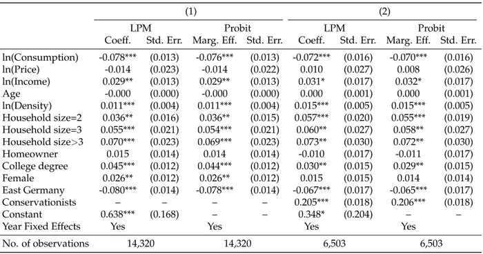
Before we examine the effects of adopting green electricity on the households’ consumption levels and quantify the response to rising electricity prices, we first identify the profile of adopters of green electricity by estimating a pooled linear probability model (LPM). The results suggest that adopting green electricity is correlated with lower consumption levels and higher incomes (Table 2). In addition, college graduates and households with a female head are more likely to subscribe. These results are in line with, for instance, Conte and Jacobsen (2016) and Kotchen and Moore (2007), and robust to estimating a nonlinear probit model rather than a LPM.

In contrast to Harding and Rapson (2017), we find that larger households are more likely to adopt green electricity. As larger household sizes indicate the presence of children, it may be that these households contribute to the private provision of emission reductions because of altruistic reasons (Clark et al., 2003). Furthermore, Table 2 shows that respondents in more densely populated areas have a higher propensity to switch to green electricity, while electricity prices do not have a significant bearing on the adoption decision.

In Panel (2) of Table 2, we use only the subsample of households that answered the question on the membership to an environmental active group and the inclination to the green party to determine the effect of being a conservationist (individuals who care about the externalities that arise through electricity generation) on the adoption of green electricity. We find that the uptake of green electricity is about 20% higher for conservationists compared to non-conservationists. Most of the remaining coefficients exhibit similar val- ues across the specifications despite the smaller and differently composed sample.

(15)

Table 2:Decision to Switch to Green Electricity Suppliers

(1) (2)

LPM Probit LPM Probit

Coeff. Std. Err. Marg. Eff. Std. Err. Coeff. Std. Err. Marg. Eff. Std. Err.

ln(Consumption) -0.078*** (0.013) -0.076*** (0.013) -0.072*** (0.016) -0.070*** (0.016)

ln(Price) -0.014 (0.023) -0.014 (0.022) 0.010 (0.027) 0.008 (0.026)

ln(Income) 0.029** (0.013) 0.029** (0.013) 0.031* (0.017) 0.032* (0.017)

Age -0.000 (0.000) -0.000 (0.000) 0.000 (0.001) 0.000 (0.001)

ln(Density) 0.011*** (0.004) 0.011*** (0.004) 0.015*** (0.005) 0.015*** (0.005) Household size=2 0.036** (0.016) 0.036** (0.015) 0.057*** (0.020) 0.055*** (0.019) Household size=3 0.055*** (0.021) 0.054*** (0.021) 0.060** (0.027) 0.058** (0.027) Household size>3 0.070*** (0.023) 0.069*** (0.023) 0.073** (0.030) 0.072** (0.030)

Homeowner 0.015 (0.014) 0.014 (0.014) -0.010 (0.017) -0.011 (0.017)

College degree 0.045*** (0.012) 0.044*** (0.012) 0.030** (0.015) 0.029** (0.015)

Female 0.026** (0.012) 0.026** (0.012) 0.015 (0.015) 0.014 (0.014)

East Germany -0.080*** (0.014) -0.078*** (0.014) -0.067*** (0.017) -0.065*** (0.017)

Conservationists – – – – 0.205*** (0.018) 0.206*** (0.018)

Constant 0.638*** (0.168) – – 0.348* (0.204) – –

Year Fixed Effects Yes Yes Yes Yes

No. of observations 14,320 14,320 6,503 6,503

Note: Standard errors are clustered at the individual level. ***, **, and * denote statistical significance at the 1 %, 5 %, and 10 % level, respectively. Asterisks on the marginal effects of the Probit model are based on the coefficients, as suggested by Greene (2007:E18-23;

2010:292).

4.1 Two-Stage Dummy Endogenous Variable Model

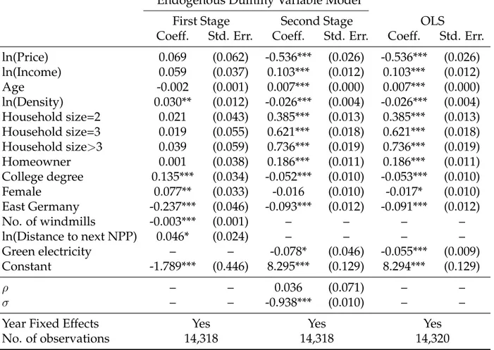
Based on the two-stage endogenous dummy variable model, we analyze whether households supplied by green electricity consume more or less electricity than households that are supplied by conventional electricity using Equations (2) and (3). Both our instrumental variables have a significant bearing on the adoption decision (see the first the estimation of the the first stage in Table 3): The likelihood to adopt green electricity decreases with the number of windmills in the neighborhood and increases with the distance to the next nuclear power plant. The second stage of the estimation procedure suggests that adopting green electricity lowers electricity consumption by about 8%.

Our finding contrasts with Harding and Rapson (2017) who detect an average increase in electricity consumption between 1-3% after subscribing to a carbon offset program and explain this negative spillover effect by moral licensing. Accordingly, the adop-

(16)

Table 3: The Effect of Adopting Green Electricity on Electricity Consumption

Endogenous Dummy Variable Model

First Stage Second Stage OLS

Coeff. Std. Err. Coeff. Std. Err. Coeff. Std. Err.

ln(Price) 0.069 (0.062) -0.536*** (0.026) -0.536*** (0.026) ln(Income) 0.059 (0.037) 0.103*** (0.012) 0.103*** (0.012)

Age -0.002 (0.001) 0.007*** (0.000) 0.007*** (0.000)

ln(Density) 0.030** (0.012) -0.026*** (0.004) -0.026*** (0.004) Household size=2 0.021 (0.043) 0.385*** (0.013) 0.385*** (0.013) Household size=3 0.019 (0.055) 0.621*** (0.018) 0.621*** (0.018) Household size>3 0.039 (0.059) 0.736*** (0.019) 0.736*** (0.019) Homeowner 0.001 (0.038) 0.186*** (0.011) 0.186*** (0.011) College degree 0.135*** (0.034) -0.052*** (0.010) -0.053*** (0.010)

Female 0.077** (0.033) -0.016 (0.010) -0.017* (0.010)

East Germany -0.237*** (0.046) -0.093*** (0.012) -0.091*** (0.012)

No. of windmills -0.003*** (0.001) – – – –

ln(Distance to next NPP) 0.046* (0.024) – – – –

Green electricity – – -0.078* (0.046) -0.055*** (0.009) Constant -1.789*** (0.446) 8.295*** (0.129) 8.294*** (0.129)

ρ – – 0.036 (0.071) – –

σ – – -0.938*** (0.010) – –

Year Fixed Effects Yes Yes Yes

No. of observations 14,318 14,318 14,320

Note: Standard errors are clustered at the individual level. ***,**, and * denote statistical significance at the 1 %, 5 %, and 10% level, respectively.

tion of one moral behavior (switching to green electricity) might induce individuals to engage in a socially undesirable or morally questionable behavior (Miller and Effron, 2010).

Yet, as suggested by the theory of positive spillover effects (Thøgersen and Crompton, 2009), our finding might reflect that the adoption of green electricity is accompanied by the motivation to engage in conserving electricity due to aiming for consistent behavior.

With respect to further covariates, we find that electricity consumption is lower in more densely populated areas, among college graduates, homeowners, and in East Ger- many. In contrast, electricity consumption increases with age and household size. To some extent, electricity consumption is additionally driven by income. A 10% increase in

(17)

income is associated with a 1% increase in electricity consumption, which is a relatively low estimate but in line with findings of Espey and Espey’s (2004) review of income elasticities.

The footer of Table 3 shows that the correlation ρ between the error terms in the selection Equation (2) and the consumption Equation (3) is rather low in magnitude and we cannot reject the null hypothesis of no correlation between them (H0 : ρ(u, ) = 0).

This indicates that selection might not be problematic, which is also suggested by the similarity to the OLS estimates.

4.2 Difference-in-Differences

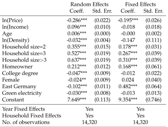
As self-selection into the treatment does not seem to be an issue, we attempt to estimate the effect of adopting green electricity by exploiting that 337 households switched from a conventional to a green electricity supplier during the sample period (Table 4).

Applying the random effects estimator to Equation (5) reveals that the reduction in electricity consumption by adopting green electricity amounts to 3%. Analogous to the previous section, electricity consumption is positively related to income, age, household size, and home ownership, but lower among households in more densely populated areas, in East Germany, as well as among households with graduated and female heads.

However, the null hypothesis of the Hausman (1978) specification test that the coefficients of the random and fixed estimator are equal is rejected (χ²(17) = 786.80, p <

0.0001). This suggests that the random effects estimator is inconsistent and that there is correlation between the explanatory variables and the individual fixed effects (Wooldridge, 2010, p. 289). Applying the fixed effects estimator renders the effect of adopting green electricity as well as other socioeconomic characteristics insignificant. Even though we cannot identify a significant effect of adopting green electricity, its coefficient exhibits the

(18)

Table 4: Difference-in-Differences Estimation Results

Random Effects Fixed Effects Coeff. Std. Err. Coeff. Std. Err.

ln(Price) -0.286*** (0.022) -0.195*** (0.026)

ln(Income) 0.096*** (0.010) -0.018 (0.018)

Age 0.006*** (0.000) -0.000 (0.002)

ln(Density) -0.032*** (0.004) -0.147 (0.111) Household size=2 0.355*** (0.015) 0.178*** (0.031) Household size=3 0.527*** (0.019) 0.267*** (0.039) Household size>3 0.637*** (0.019) 0.310*** (0.039) Homeowner 0.212*** (0.012) 0.168*** (0.061) College degree -0.047*** (0.009) -0.012 (0.022)

Female -0.024** (0.009) 0.024 (0.040)

East Germany -0.102*** (0.011) 0.482*** (0.064) Green electricity -0.030*** (0.008) -0.013 (0.013)

Constant 7.649*** (0.113) 9.354*** (0.746)

Year Fixed Effects Yes Yes

Household Fixed Effects Yes Yes

No. of observations 14,320 14,320

Note: Standard errors are clustered at the individual level. ***, **, and * denote statistical significance at the 1 %, 5 %, and 10 % level, respectively.

same sign as in the random effects estimation.

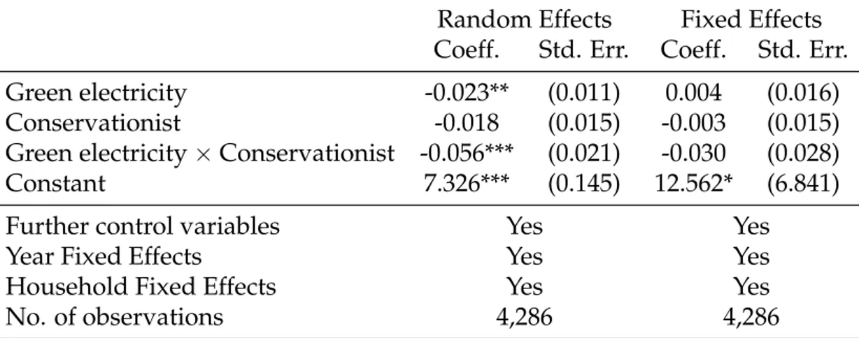
To test Kotchen and Moore’s (2008) hypothesis of heterogeneous effects of subscribing to green electricity across conservationists and non-conservationists, we analyze the subsample of households that participated in the last three survey waves where additional questions concerning environmental attitudes were asked. The random effects estimation results reported in Table 5 indicate that there is no difference in the consumption level between conservationists and non-conservationists who are supplied by conventional electricity. After adopting green electricity, non-conservationists reduce their electricity consumption by 2.3%, which is in line with Kotchen and Moore (2008).

Yet, in contrast to these authors, we observe that also conservationists lower their electricity demand after adopting green electricity. However, this interaction effect be-

(19)

Table 5: Difference-in-Differences Estimation Results Including an Interaction Term for Conservationists

Random Effects Fixed Effects Coeff. Std. Err. Coeff. Std. Err.

Green electricity -0.023** (0.011) 0.004 (0.016)

Conservationist -0.018 (0.015) -0.003 (0.015)

Green electricity×Conservationist -0.056*** (0.021) -0.030 (0.028)

Constant 7.326*** (0.145) 12.562* (6.841)

Further control variables Yes Yes

Year Fixed Effects Yes Yes

Household Fixed Effects Yes Yes

No. of observations 4,286 4,286

Note: Standard errors are clustered at the individual level. ***, **, and * denote statistical significance at the 1 %, 5 %, and 10 % level, respectively. For the sake of brevity all remaining regressors are omitted.

comes insignificant when we apply the fixed-effects estimator. This might be due to the fact that as little as 53 individuals changed their conservationist status during the survey period. Exploiting this little within-variation, we fail to identify the negative effect of switching to green electricity for both conservationists and non-conservationists.

4.3 Price Elasticity

The previous sections indicate that switching to green electricity has a negative bearing on electricity consumption. This result might be driven by two factors. First, households may exhibit positive spillover effects and consume less electricity after adopting green electricity due to the desire for consistent behavior. Second, green electricity is on average more expensive, which might result in a lower consumption of electricity if green electricity households react to price increases. To disentangle these two effects, in follows, we estimate the price elasticity for households supplied by green and conventional electricity, respectively.

(20)

Therefore, we estimate the price elasticity for consumers of green and conventional electricity separately, without correcting for self-selection using standard panel estimation methods (Table 6). The null hypothesis of Hausman’s (1978) specification test that there is no correlation between the explanatory variables and the individual fixed effects can be rejected for both consumers of green electricity (χ²(15) = 160.4, p < 0.0001) and conventional electricity (χ²(16) = 526.7, p <0.0001). Applying the fixed effects estimator yields price elasticity of around -0.2.⁵

Table 6:Random Effects Model of the Price Elasticity

Random Effects Fixed Effects

Conventional Green Conventional Green

Coeff. Std. Err. Coeff. Std. Err. Coeff. Std. Err. Coeff. Std. Err.

ln(Price) -0.289*** (0.030) -0.302*** (0.036) -0.193*** (0.035) -0.220*** (0.044) ln(Income) 0.102*** (0.013) 0.074*** (0.019) -0.032 (0.025) -0.049 (0.031)

Age 0.006*** (0.000) 0.006*** (0.001) 0.000 (0.001) 0.001 (0.002)

ln(Density) -0.028*** (0.004) -0.037*** (0.006) -0.091 (0.134) -0.246 (0.182) Household size=2 0.356*** (0.018) 0.357*** (0.027) 0.152*** (0.040) 0.212*** (0.058) Household size=3 0.528*** (0.022) 0.560*** (0.035) 0.224*** (0.045) 0.353*** (0.079) Household size>3 0.654*** (0.023) 0.615*** (0.033) 0.281*** (0.048) 0.333*** (0.074) Homeowner 0.213*** (0.014) 0.227*** (0.022) 0.083 (0.068) 0.351** (0.154) College degree -0.038*** (0.012) -0.061*** (0.015) -0.017 (0.032) -0.009 (0.031)

Female -0.017 (0.011) -0.033** (0.016) -0.009 (0.028) -0.032 (0.043)

East Germany -0.108*** (0.013) -0.087*** (0.022) 0.575*** (0.072) 0.000 (.) Constant 7.584*** (0.146) 7.842*** (0.187) 9.138*** (0.895) 10.162*** (1.234)

Year Fixed Effects Yes Yes Yes Yes

Household Fixed Effects Yes Yes Yes Yes

No. of observations 9,550 4,770 9,550 4,770

Note: Standard errors are clustered at the individual level. ***,**, and * denote statistical significance at the 1 %, 5 %, and 10% level, respectively. Standard errors for the long-run elasticities are computed using the delta method (Greene, 2003, p. 68).

Hence, the response to price increases is substantially lower than the estimated effect of switching to green electricity (Table 4) would suggest. Given that the electricity price of households with green tariffs is only about 1.6% higher (Table 1), a 3% (1.3%) reduction in electricity consumption would result in a price elasticity of around -1.9 (-0.81). This

5A more sophisticated analysis of the price elasticity requires the estimation of a dynamic model that incorporates the lagged term of the dependent variable. The proper identification of such a model requires that households report their electricity consumption at leastT = 4, but this only holds for 392 households in our sample. Moreover, one would need to correct for the endogeneity of the price variable (Taylor et al., 2004). For an application, we refer the reader to Frondel et al. (2018).

(21)

comparison provides tentative evidence that the reaction of households adopting green electricity is larger than implied by price increases. Consequently, households with green tariffs reduce their consumption for other reasons than prices and may exhibit a positive spillover effect.

5 Conclusion

Using panel data on about 9,000 households, this paper has identified the profile of households that adopt green electricity, has analyzed the impact of adopting green electricity on consumption, and has quantified the response to rising electricity prices.

Recognizing that the decision to adopt green electricity and the consumption level might be jointly influenced by unobservable factors, we account for potential self-selection by employing a dummy endogenous variable model (Heckman, 1976, 1978).

We find that the typical adopter of green electricity is wealthier and better educated than the typical user of conventional electricity and lives in a larger household. This has important implications for the marketing of green electricity programs. Green electricity program will experience higher participation rates and result in lower marketing expenditures if they are targeted at households that are most likely to adopt green electricity (Kotchen and Moore, 2007; Conte and Jacobsen, 2016).

Moreover, we detect that households – particularly those who care about the externalities of electricity consumption – switching to green electricity consume less electricity compared to users of conventional electricity. This effect is substantially larger than the estimated price elasticity for households with green tariffs would imply. Hence, households that adopt green electricity reduce electricity for other reasons than prices. We interpret this as tentative evidence for a positive spillover effect from the adoption of green

(22)

electricity that arises through the desire of a consistent behavior.

As households that stick to conventional electricity exhibit a relatively high price elasticity, one potential way to reduce the negative externalities from electricity generation is to increase the price for conventional electricity. Although additional pecuniary measures for conventional electricity would lower the consumption (and emissions) of the affected customers, from a global perspective, the bearing on greenhouse gas emissions is hazy because of Germany’s participation in the European Emissions Trading Scheme (Frondel et al., 2010). The lower demand for electricity generated by fossil plants would lead to a decrease in the demand for allowances, which in turn could be purchased at lower prices by other companies that participate in the scheme. Thus, carbon emissions could only be effectively reduced if the corresponding allowances were to be eliminated.

(23)

A Appendix

Table A1:Comparison to the population of German household heads

Variable Our sample Household heads in

Germany (2011-2016)

Age below 35 years 0.050 0.194

Age between 35 and 64 years 0.773 0.525

Age above 65 years 0.177 0.281

Income>e4,500 0.107 0.107

Household Size = 1 0.229 0.407

Household Size≥4 0.142 0.126

Homeowner 0.664 0.465

College degree 0.266 0.190

Female 0.356 0.353

East Germany 0.213 0.210

Source: Destatis (2017a) and Destatis (2017b).

References

Andor, M. A., Frondel, M., and Vance, C. (2017). Germany’s Energiewende: A tale of increasing costs and decreasing willingness-to-pay. Energy Journal, 38(SI 1):211–228.

Angrist, J. D., Imbens, G. W., and Rubin, D. B. (1996). Identification of causal effects using instrumental variables. Journal of the American Statistical Association, 91(434):444–455.

Blanken, I., van de Ven, N., and Zeelenberg, M. (2015). A meta-analytic review of moral licensing. Personality and Social Psychology Bulletin, 41(4):540–558.

BNetzA (2018). Übersicht Stromnetzbetreiber Stand 09.05.2018. Bundesnetzagentur, Bonn.

Borenstein, S. (2009). To what electricity price do consumers respond? Residential demand elasticity under increasing-block pricing. Preliminary Draft April.

Clark, C. F., Kotchen, M. J., and Moore, M. R. (2003). Internal and external influences

(24)

on pro-environmental behavior: Participation in a green electricity program. Journal of Environmental Psychology, 23(3):237–246.

Conte, M. N. and Jacobsen, G. D. (2016). Explaining demand for green electricity using data from all US utilities. Energy Economics, 60:122–130.

Destatis (2017a). Bevölkerung und Erwerbstätigkeit. Haushalte und Familien. Ergebnisse des Mikrozensus. Statistisches Bundesamt, Berlin. URL https://www.destatis.

de/GPStatistik/receive/DESerie_serie_00000209. Accessed: 04-24-2018.

Destatis (2017b). Wirtschaftsrechnungen. Laufende Wirtschaftsrechnungen. Einkommen, Einnahmen und Ausgaben privater Haushalte. Statistisches Bundesamt, Berlin.

URL https://www.destatis.de/GPStatistik/receive/DESerie_serie_

00000152. Accessed: 04-24-2018.

Dietz, T., Ostrom, E., and Stern, P. C. (2003). The struggle to govern the commons.Science, 302(5652):1907–1912.

Dolan, P. and Galizzi, M. M. (2015). Like ripples on a pond: Behavioral spillovers and their implications for research and policy. Journal of Economic Psychology, 47:1–16.

Ebeling, F. and Lotz, S. (2015). Domestic uptake of green energy promoted by opt-out tariffs. Nature Climate Change, 5:868–871.

Espey, J. A. and Espey, M. (2004). Turning on the lights: A meta-analysis of residential electricity demand elasticities. Journal of Agricultural and Applied Economics, 36(01):65–

81.

Frondel, M., Kussel, G., and Sommer, S. (2018). The price response of residential electricity demand in Germany: A dynamic approach. SFB 823 Discussion Papers # 13/2018.

Frondel, M., Ritter, N., Schmidt, C. M., and Vance, C. (2010). Economic impacts from the

(25)

promotion of renewable energy technologies: The German experience. Energy Policy, 38(8):4048–4056.

Greene, W. (2007). Limdep Version 9.0 Econometric Modeling Guide. New York: Econo- metric Software.

Greene, W. (2010). Testing hypotheses about interaction terms in nonlinear models. Eco- nomics Letters, 107(2):291–296.

Greene, W. H. (2003). Econometric analysis. Pearson Education India.

Harding, M. and Rapson, D. (2017). Do voluntary carbon offsets induce energy rebound?

A conservationist’s dilemma. Working Paper.

Hausman, J. A. (1978). Specification tests in econometrics. Econometrica: Journal of the Econometric Society, pages 1251–1271.

He, X. and Reiner, D. (2017). Why consumers switch energy suppliers: The role of individual attitudes. Energy Journal, 38(6).

Heckman, J. J. (1976). The common structure of statistical models of truncation, sample selection and limited dependent variables and a simple estimator for such models. In Annals of Economic and Social Measurement, Volume 5, Number 4, pages 475–492. NBER, Cambridge.

Heckman, J. J. (1978). Dummy endogenous variables in a simultaneous equation system.

Econometrica, 46(4):931–959.

Hobman, E. V. and Frederiks, E. R. (2014). Barriers to green electricity subscription in Australia: ”Love the environment, love renewable energy . . . but why should I pay more?”. Energy Research & Social Science, 3:78–88.

(26)

Hortaçsu, A., Madanizadeh, S. A., and Puller, S. L. (2017). Power to choose? An analysis of consumer inertia in the residential electricity market. American Economic Journal:

Economic Policy, 9(4):192–226.

Ito, K. (2014). Do consumers respond to marginal or average price? evidence from nonlinear electricity pricing. American Economic Review, 104(2):537–563.

Jacobsen, G. D., Kotchen, M. J., and Vandenbergh, M. P. (2012). The behavioral response to voluntary provision of an environmental public good: Evidence from residential electricity demand. European Economic Review, 56(5):946–960.

Kotchen, M. J. and Moore, M. R. (2007). Private provision of environmental public goods:

Household participation in green-electricity programs. Journal of Environmental Eco- nomics and Management, 53(1):1–16.

Kotchen, M. J. and Moore, M. R. (2008). Conservation: From voluntary restraint to a voluntary price premium. Environmental and Resource Economics, 40(2):195–215.

Maddala, G. S. (1983). Limited-dependent and qualitative variables in econometrics. Cam- bridge: Cambridge University Press.

Merritt, A. C., Effron, D. A., and Monin, B. (2010). Moral self-licensing: When being good frees us to be bad. Social and Personality Psychology Compass, 4(5):344–357.

Miller, D. T. and Effron, D. A. (2010). Psychological license: When it is needed and how it functions. In Advances in experimental social psychology, volume 43, pages 115–155.

Amsterdam: Elsevier.

Olofsson, A. and Öhman, S. (2006). General beliefs and environmental concern: Transat- lantic comparisons. Environment and Behavior, 38(6):768–790.

PEW (2015). Global concern about climate change, broad support for limiting emissions.

PEW Research Center.

(27)

RWI and forsa (2015). The German Residential Energy Consumption Survey 2011 - 2013, Study commissioned by the German Ministry for Economics and Energy (BMWi).

Sundt, S. and Rehdanz, K. (2015). Consumers’ willingness to pay for green electricity: A meta-analysis of the literature. Energy Economics, 51:1–8.

Sunstein, C. R. and Reisch, L. A. (2014). Automatically green: Behavioral economics and environmental protection. Harvard Environmental Law Review, 38:127.

Taylor, R. G., McKean, J. R., and Young, R. A. (2004). Alternate price specifications for estimating residential water demand with fixed fees. Land Economics, 80(3):463–475.

Thøgersen, J. and Crompton, T. (2009). Simple and painless? The limitations of spillover in environmental campaigning. Journal of Consumer Policy, 32(2):141–163.

Tiefenbeck, V., Staake, T., Roth, K., and Sachs, O. (2013). For better or for worse? Empir- ical evidence of moral licensing in a behavioral energy conservation campaign. Energy Policy, 57:160–171.

Truelove, H. B., Carrico, A. R., Weber, E. U., Raimi, K. T., and Vandenbergh, M. P. (2014).

Positive and negative spillover of pro-environmental behavior: An integrative review and theoretical framework. Global Environmental Change, 29:127–138.

UBA (2015). Daten zur Umwelt: Umwelt, Haushalte und Konsum. Umweltbundesamt, Berlin.

WEC (2017). Average electricity consumption per electrified household. World Energy Council, London. URL https://www.wec-indicators.enerdata.eu/

household-electricity-use.html. Accessed: 04-24-2018.

Wooldridge, J. M. (2010). Econometric analysis of cross section and panel data. MIT press.

(28)

(29)

(30)