Heidelberger Numerikbibliothek für die Lehre

(1)

für die Lehre

Peter Bastian Universität Heidelberg

Interdisziplinäres Zentrum für Wissenschaftliches Rechnen Im Neuenheimer Feld 368, D-69120 Heidelberg

email: Peter.Bastian@iwr.uni-heidelberg.de 20. Oktober 2013

Die Heidelberger Numerikbibliothek wurde begleitend zu den Vorlesungen Einführung in die Numerik und Numerik in der Programmiersprache C++

entwickelt und stellt einfach zu benutzende Klassen für grundlegende Aufga- ben in der Numerik bis hin zur Lösung von gewöhnlichen Differentialgleichun- gen zur Verfügung. In fast allen Klassen ist der benutzte Zahlentyp parame- trisierbar so dass auch hochpräzise Rechnungen durchgeführt werden können.

Inhaltsverzeichnis

1 Einführung

Was ist HDNUM

• HDNUM ist eine kleine Sammlung von C++ Klassen, die die Implementierung numerischer Algorithmen aus der Vorlesung erleichtern soll.

• Die aktuelle Version gibt es unter

http://conan.iwr.uni-heidelberg.de/teaching/numerik1_ws2011/

• Einige Ziele bei der Entwicklung von HDNUM waren:

(2)

– Einfache Installation: Es mur nur eine Header-Datei eingebunden werden.

– Einfache Benutzung der Klassen: Z.B. keine dynamische Speicherverwaltung.

– Möglichkeit der Rechnung mit verschiedenen Zahl-Datentypen.

– Effiziente Realisierung der Verfahren möglich: Z.B. Block-Algorithmen in der linearen Algebra.

Installation

• Dateihdnum-x.yy.tgz (komprimiertes tar archive) herunterladen.

• Archiv mit tar zxf hdnum-x.yy.tgz entpacken.

• Das Verzeichnis enthält unter anderem:

– Das Verzeichnis src mit dem Quellcode der Klassen (muss Sie nicht interes- sieren).

– Das Verzeichnis examples mit den Beispielanwendungen (die sollten Sie sich ansehen).

– Das Verzeichnis tutorial: Quelle für dieses Dokument.

– Die Dateihdnum.hh, die zentrale Header-Datei, die in alle Anwendungen eingebunden werden muss.

• Das Verzeichnis hdnum/examples enthält ein simples Makefile zum Übersetzen der Programme.

• Die Beispiele erfordern die Installation der GNU multiprecision libraryhttp://gmplib.org/.

Ist diese nicht vorhanden müssen Makefiles entsprechend angepasst werden.

Typisches HDNUM Programm

1 // hallohdnum . cc

2 # include < iostream > // n o t w e n d i g z u r Ausgabe

3 # include < vector >

4 # include " hdnum . hh " // hdnum h e a d e r

5

6 int main ()

7 {

8 hdnum :: Vector <float> a (10 ,3.14); // F e l d mit 10 i n i t . Elementen

9 a [3] = 1.0; // Z u g r i f f a u f Element 3

10 }

• Übersetzen im Verzeichnisexamples mit GMP installiert:

g++ -I.. -o hallohdnum hallohdnum.cc -lm -lgmpxx -lgmp

• und ohne GMP:

g++ -I.. -o hallohdnum hallohdnum.cc -lm

(3)

• oder einfach

make

• oder falls kein GMP installiert ist

make nogmp

2 Ein kleiner Programmierkurs

2.1 Hallo Welt

Programmierumgebung

• Wir benutzen die Programmiersprache C++.

• Wir behandeln nur die Programmierung unter LINUX mit den GNU compilern.

• Windows: On your own.

• Wir setzen Grundfertigkeit im Umgang mit LINUX-Rechnern voraus:

– Shell, Kommandozeile, Starten von Programmen.

– Dateien, Navigieren im Dateisystem.

– Erstellen von Textdatein mit einem Editor ihrer Wahl.

• Idee des Kurses: „Lernen an Beispielen“, keine rigorose Darstellung.

• Blutige Anfänger sollten zusätzlich ein Buch lesen (siehe Literaturliste).

Workflow

C++ ist eine „kompilierte“ Sprache. Um ein Programm zur Ausführung zu bringen sind folgende Schritte notwendig:

1. Erstelle/Ändere den Programmtext mit einem Editor.

2. Übersetze den Programmtext mit dem C++-Übersetzer (auch C++-Compiler) in ein Maschinenprogramm.

3. Führe das Programm aus. Das Programm gibt sein Ergebnis auf dem Bildschirm oder in eine Datei aus.

4. Interpretiere Ergebnisse. Dazu benutzen wir weitere Programme wie gnuplotoder grep.

5. Falls Ergebnis nicht korrekt, gehe nach 1!

(4)

HDNUM

• C++ kennt keine Matrizen, Vektoren, Polynome, . . .

• Wir haben C++ erweitert um dieHeidelberg Educational Numerics Library, kurzHDNum.

• Alle in der Vorlesung behandelten Beispiele sind dort enthalten.

Herunterladen von HDNUM 1. Einloggen

2. Erzeuge neues Verzeichnis mit $ mkdir kurs 3. Wechsle in das Verzeichnis mit $ cd kurs

4. Gehe zur Webseite http://conan.iwr.uni-heidelberg.de/teaching/numerik1_ws2013/index.html

5. Klicke auf Version 0.25 und bestätige

6. Kopiere Dateihdnum-0.25.tgzin das Verzeichnis: $ cp ~/Desktop/hdnum-0.25.tgz . 7. Entpacken der Datei mit $ tar zxvf hdnum-0.25.tgz

8. Wechsle in das Verzeichnis $ cd hdnum/examples 9. Anzeigen der Dateien mittels $ ls

Wichtige UNIX-Befehle

• ls --color -F - Zeige Inhalt des aktuellen Verzeichnisses

• cd - Wechsle ins Home-Verzeichnis

• cd <verzeichnis>- Wechsle in das angegebene Verzeichnis (im aktuellen Verzeich- nis)

• cd .. - Gehe aus aktuellem Verzeichnis heraus

• mkdir < verzeichnis> - Erstelle neues Verzeichnis

• cp <datei1> <datei2> - Kopiere datei1 auf datei2 (datei2 kann durch Verzeichnis ersetzt werden)

• mv <datei1> <datei2> - Benenne datei1 in datei2 um (datei2 kann durch Ver- zeichnis ersetzt werden, dann wird datei1 dorthin verschoben)

• rm <datei> - Lösche datei

• rm -rf <verzeichnis> - Lösche Verzeichnis mit allem darin

(5)

Hallo Welt !

Öffne die Datei hallowelt.ccmit einem Editor: $ gedit hallowelt.cc

1 // h a l l o w e l t . cc ( Dateiname a l s Kommentar )

2 # include < iostream > // n o t w e n d i g z u r Ausgabe

3

4 int main ()

5 {

6 std :: cout << " Numerik ␣ 0 ␣ ist ␣ leicht : " << std :: endl ;

7 std :: cout << " 1+1= " << 1+1 << std :: endl ;

8 }

• iostream ist eine sog. „Headerdatei“

• #include erweitert die „Basissprache“.

• int main ()braucht man immer: „Hier geht’s los“.

• { ... }klammert Folge von Anweisungen.

• Anweisungen werden durch Semikolon abgeschlossen.

Hallo Welt laufen lassen

• Gebe folgende Befehle ein:

$ g ++ -o h a l l o w e l t h a l l o w e l t . cc

$ ./ h a l l o w e l t

• Dies sollte dann die folgende Ausgabe liefern:

Numerik 0 ist ganz leicht : 1+1=2

2.2 Variablen und Typen (Zahl-) Variablen

• Aus der Mathematik: „x ∈ M“. Variable x nimmt einen beliebigen Wert aus der Menge M an.

• Geht in C++ mit: M x;

• Variablendefinition: x ist eine Variable vom Typ M.

• Mit Initialisierung: M x(0);

• Wert von Variablen der „eingebauten“ Typen ist sonst nicht definiert.

(6)

1 // z a h l e n . cc

2 # include < iostream >

3 int main ()

4 {

5 u n s i g n e d int i ; // u n i n i t i a l i s i e r t e n a t ü r l i c h e Z a h l

6 double x (3.14); // i n i t i a l i s i e r t e Fließkommazahl

7 float y (1.0); // e i n f a c h e G e n a u i g k e i t

8 short j (3); // e i n e " k l e i n e " Z a h l

9 std :: cout << " ( i + x )*( y + j )= " << ( i + x )*( y + j ) << std :: endl ;

10 }

Andere Typen

• C++ kennt noch viele weitere Typen.

• Typen können nicht nur Zahlen sondern viele andere Informationen repräsentieren.

• Etwa Zeichenketten: std::string

• Oft muss man dazu weitere Headerdateien angeben.

1 // s t r i n g . cc

3 # include < string >

4 int main ()

5 {

6 std :: string m1 ( " Zeichen " );

7 std :: string leer ( " ␣ ␣ ␣ " );

8 std :: string m2 ( " kette " );

9 std :: cout << m1 + leer + m2 << std :: endl ;

10 }

• Jede Variablemuss einen Typ haben. Strenge Typbindung.

Mehr Zahlen

1 // mehrzahlen . cc

2 # include < iostream > // h e a d e r f ü r Ein−/Ausgabe

3 # include < complex > // h e a d e r f ü r komplexe Zahlen

4 int main ()

5 {

6 std :: complex <double> y (1.0 ,3.0);

7 std :: cout << y << std :: endl ;

8 }

• GNU Multiprecision Library http://gmplib.org/ erlaubt Zahlen mit vielen Stel- len (hier 512 Stellen zur Basis 2).

• Übersetzen mit: $ g++ -o mehrzahlen mehrzahlen.cc -lgmpxx -lgmp

• Komplexe Zahlen sind Paare von Zahlen.

• complex<> ist ein Template: Baue komplexe Zahlen aus jedem anderen Zahlentyp auf (später mehr!).

(7)

Mehr Ein- und Ausgabe

1 // e i n g a b e . cc

3 # include < iomanip > // f ü r s e t p r e c i s i o n

4 # include < cmath > // f ü r s q r t

5 int main ()

6 {

7 double x (0.0);

8 std :: cout << " Gebe ␣ eine ␣ Zahl ␣ ein : ␣ " ;

9 std :: cin >> x ;

10 std :: cout << " Wurzel ( x )= ␣ "

11 << std :: s c i e n t i f i c << std :: s h o w p o i n t

12 << std :: s e t p r e c i s i o n (15)

13 << sqrt ( x ) << std :: endl ;

14 }

• Eingabe geht mit std::cin >> x;

• Standardmäßig werden nur 6 Nachkommastellen ausgegeben. Das ändert man mit std::setprecision.

• Dazu muss man die Headerdateiiomanip einbinden.

• Die Wurzel berechnet die Funktionsqrt.

Zuweisung

• Den Wert von Variablen kann man ändern. Sonst wäre es langweilig :-)

• Dies geht mittels Zuweisung:

double x (3.14); // V a r i a b l e n d e f i n i t i o n mit I n i t i a l i s i e r u n g double y ; // u n i n i t i a l i s i e r t e V a r i a b l e

y = x ; // Weise y den Wert von x zu

x = 2.71; // Weise x den Wert 2 . 7 1 , y u n v e r ä n d e r t y = ( y *3)+4; // Werte Ausdruck r e c h t s von = aus

// und w e i s e das R e s u l t a t y zu !

Blöcke

• Block: Sequenz von Variablendefinitionen und Zuweisungen in geschweiften Klam- mern.

{

double x (3.14);

double y ; y = x ; }

• Blöcke können rekursiv geschachtelt werden.

• Eine Variable ist nur in dem Block sichtbar in dem sie definiert ist sowie in allen darin enthaltenen Blöcken:

(8)

{

double x (3.14);

{

double y ; y = x ; }

y = ( y *3)+4; // g e h t n i c h t , y n i c h t mehr s i c h t b a r . }

Whitespace

• Das Einrücken von Zeilen dient der besseren Lesbarkeit, notwendig ist es (fast) nicht.

• #include-Direktiven müssen immer einzeln auf einer Zeile stehen.

• Ist das folgende Programm lesbar?

1 // w h i t e s p a c e . cc

2 # include < iostream > // i n c l u d e s a u f e i g e n e r Z e i l e !

3 # include < iomanip >

4 # include < cmath >

5 int main (){double x (0.0);

6 std :: cout < < " Gebe ␣ eine ␣ lange ␣ Zahl ␣ ein : ␣ " ; std :: cin >> x ;

7 std :: cout < < " Wurzel ( x )= ␣ " << std :: scientific < < std :: s h o w p o i n t

8 << std :: s e t p r e c i s i o n (16) < < sqrt ( x ) < < std :: endl ;}

2.3 Entscheidung If-Anweisung

• Aus der Mathematik kennt man eine „Zuweisung“ der folgenden Art.

Für x∈Rsetze

y=|x|=

x falls x≤0

−x sonst

• Dies realisiert man in C++ mit einerIf-Anweisung:

double x (3.14) , y ; if (x >=0)

{

y = x ; }

else {

y = -x ; }

(9)

Varianten der If-Anweisung

• Die geschweiften Klammern kann man weglassen, wenn der Block nur eine Anwei- sung enthält:

double x (3.14) , y ;

if (x >=0) y = x ; else y = -x ;

• Der else-Teil ist optional:

double x =3.14;

if (x <0)

std :: cout << " x ␣ ist ␣ negativ ! " << std :: endl ;

• Weitere Vergleichsoperatoren sind< <= == >= > !=

• Beachte: = für Zuweisung, aber == für den Vergleich zweier Objekte!

2.4 Wiederholung While-Schleife

• Bisher: Sequentielle Abfolge von Befehlen wie im Programm angegeben. Das ist langweilig :-)

• Eine Möglichkeit zur Wiederholung bietet die While-Schleife:

while ( Bedingung ) { Schleifenkörper }

• Beispiel:

int i =0; while (i <10) { i = i +1; }

• Bedeutung:

1. Teste Bedingung der While-Schleife

2. Ist diesewahr dann führe Anweisungen im Schleifenkörper aus, sonst gehe zur ersten Anweisung nach dem Schleifenkörper.

3. Gehe nach 1.

• Anweisungen im Schleifenkörper beeinflussen normalerweise den Wahrheitswert der Bedingung.

• Endlosschleife: Wert der Bedingung wird niefalsch.

(10)

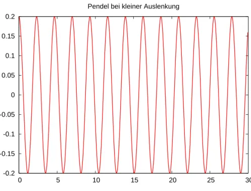
Pendel (analytische Lösung; while-Schleife)

• Die Auslenkung des Pendels mit der Näherungsin(φ)≈φund φ(0) =φ0, φ^′(0) = 0 lautet:

φ(t) = φ0cos rg

l

.

• Das folgende Programm gibt diese Lösung zu den Zeiten tⁱ = i∆t, 0 ≤ tⁱ ≤ T, i∈N₀ aus:

1 // p e n d e l w h i l e . cc

3 # include < cmath > // mathematische Funktionen

4 int main ()

5 {

6 double l (1.34); // P e n d e l l ä n g e i n Meter

7 double phi0 (0.2); // Amplitude im Bogenmaß

8 double dt (0.05); // Z e i t s c h r i t t i n Sekunden

9 double T (30.0); // Ende i n Sekunden

10 double t (0.0); // Anfangswert

11

12 while ( t <= T )

13 {

14 std :: cout << t << " ␣ "

15 << phi0 * cos ( sqrt (9.81/ l )* t )

16 << std :: endl ;

17 t = t + dt ;

18 }

19 }

Wiederholung (for-Schleife)

• Möglichkeit der Wiederholung: for-Schleife:

for ( Anfang; Bedingung; Inkrement) { Schleifenkörper }

• Beispiel:

for (int i =0; i <=5; i = i +1) {

std :: cout << " Wert ␣ von ␣ i ␣ ist ␣ " << i << std :: endl ; }

• Enthält der Block nur eine Anweisung dann kann man die geschweiften Klammern weglassen.

• Die Schleifenvariable ist so nur innerhalb des Schleifenkörpers sichtbar.

• Die for-Schleife kann auch mittels einerwhile-Schleife realisiert werden.

(11)

-0.2 -0.15 -0.1 -0.05 0 0.05 0.1 0.15 0.2

0 5 10 15 20 25 30

Pendel bei kleiner Auslenkung

Abbildung 1: Das Pendel in Aktion. Gnuplot-Ausgabe des Programmes pendel.cc.

Pendel (analytische Lösung, for-Schleife)

1 // p e n d e l . cc

4 int main ()

5 {

7 double phi0 (0.2); // Amplitude im Bogenmaß

8 double dt (0.05); // Z e i t s c h r i t t i n Sekunden

10 for (double t =0.0; t <= T ; t = t + dt )

11 {

12 std :: cout << t << " ␣ "

13 << phi0 * cos ( sqrt (9.81/ l )* t )

14 << std :: endl ;

15 }

16 }

Visualisierung mit Gnuplot

• Gnuploterlaubt einfache Visualisierung von Funktionenf :R→Rundg :R×R→ R.

• Fürf :R→Rgenügt eine zeilenweise Ausgabe von Argument und Funktionswert.

• Umlenken der Ausgabe eines Programmes in eine Datei:$ ./pendel > pendel.dat$

(12)

• Starte gnuplot gnuplot> plot "pendel.dat"with lines Geschachtelte Schleifen

• Ein Schleifenkörper kann selbst wieder eine Schleife enthalten, man spricht von geschachtelten Schleifen.

• Beispiel:

for (int i =1; i <=10; i = i +1) for (int j =1; j <=10; j = j +1)

if ( i == j )

std :: cout << " i ␣ gleich ␣ j : ␣ " << std :: endl ; else

std :: cout << " i ␣ u n g l e i c h ␣ j ! " << std :: endl ;

Numerische Lösung des Pendels

• Volles Modell für das Pendel aus der Einführung:

d²φ(t) dt² =−g

l sin(φ(t)) ∀t >0, φ(0) =φ0, dφ

dt(0) =u0.

• Umschreiben in System erster Ordnung:

dφ(t)

dt =u(t), d²φ(t)

dt² = du(t) dt =−g

l sin(φ(t)).

• Eulerverfahren fürφⁿ=φ(n∆t), uⁿ =u(n∆t):

φⁿ⁺¹ =φⁿ+ ∆t uⁿ φ⁰ =φ0

uⁿ⁺¹ =uⁿ−∆t(g/l) sin(φⁿ) u⁰ =u0

Pendel (expliziter Euler)

1 // p e n d e l n u m e r i s c h . cc

4

5 int main ()

6 {

8 double phi (3.0); // A n f a n g s a m p l i t u d e i n Bogenmaß

9 double u (0.0); // A n f a n g s g e s c h w i n d i g k e i t

10 double dt (1 E -4); // Z e i t s c h r i t t i n Sekunden

12 double t (0.0); // A n f a n g s z e i t

13

14 std :: cout << t << " ␣ " << phi << std :: endl ;

(13)

15 while (t < T )

16 {

17 t = t + dt ; // i n k r e m e n t i e r e Z e i t

18 double phialt ( phi );// merke p h i

19 double ualt ( u ); // merke u

20 phi = phialt + dt * ualt ; // neues p h i

21 u = ualt - dt *(9.81/ l )* sin ( phialt );// neues u

23 }

24 }

2.5 Funktionen

Funktionsaufruf und Funktionsdefinition

• In der Mathematik gibt es das Konzept derFunktion.

• In C++ auch.

• Sei f :R→R, z.B. f(x) = x².

• Wir unterscheiden den Funktionsaufruf

double x , y ; y = f ( x );

• und dieFunktionsdefinition. Diese sieht so aus:

Ergebnistyp Funktionsname ( Argumente ) { Funktionsrumpf }

• Beispiel:

double f (double x ) {

return x * x ; }

Komplettbeispiel zur Funktion

1 // f u n k t i o n . cc

3

4 double f (double x )

5 {

6 return x * x ;

7 }

8

9 int main ()

10 {

11 double x (2.0);

12 std :: cout << " f ( " << x << " )= " << f ( x ) << std :: endl ;

13 }

(14)

• Funktionsdefinition muss vor Funktionsaufruf stehen.

• Formales Argument in der Funktionsdefinition entspricht einer Variablendefinition.

• Beim Funktionsaufruf wird das Argument (hier) kopiert.

• main ist auch nur eine Funktion.

Weiteres zum Verständnis der Funktion

• Der Name des formalen Arguments in der Funktionsdefinition ändert nichts an der Semantik der Funktion (Sofern es überall geändert wird):

double f (double y ) {

return y * y ; }

• Das Argument wird hier kopiert, d.h.:

double f (double y ) {

y = 3* y * y ; return y ; }

int main () {

double x (3.0) , y ;

y = f ( x ); // ä n d e r t n i c h t s an x ! }

Weiteres zum Verständnis der Funktion

• Argumentliste kann leer sein (wie in der Funktionmain):

double pi () {

return 3.14;

}

y = pi (); // Klammern s i n d e r f o r d e r l i c h !

• Der Rückgabetyp void bedeutet „keine Rückgabe“

void hello () {

std :: cout << " hello " << std :: endl ; }

hello ();

• Mehrere Argument werden durch Kommata getrennt:

double g (int i , double x ) {

return i * x ; }

std :: cout << g (2 ,3.14) << std :: endl ;

(15)

Pendelsimulation als Funktion

1 // p e n d e l m i t f u n k t i o n . cc

4

5 void s i m u l i e r e _ p e n d e l (double l , double phi , double u )

6 {

7 double dt = 1E -4;

8 double T = 30.0;

9 double t = 0.0;

10

12 while (t < T )

13 {

14 t = t + dt ;

15 double phialt ( phi ) , ualt ( u );

16 phi = phialt + dt * ualt ;

17 u = ualt - dt *(9.81/ l )* sin ( phialt );

19 }

20 }

21

22 int main ()

23 {

25 double phi (3.0);// A n f a n g s a m p l i t u d e i n Bogenmaß

26 double u (0.0); // A n f a n g s g e s c h w i n d i g k e i t

27 s i m u l i e r e _ p e n d e l (l , phi , u );

28 }

Funktionsschablonen

• Oft macht eine Funktion mit Argumenten verschiedenen Typs einen Sinn.

• double f (double x) {return x*x;}macht auch mitfloat,intodermpf_class Sinn.

• Man könnte die Funktion für jeden Typ definieren. Das ist natürlich sehr umständ- lich. (Es darf mehrere Funktionen gleichen Namens geben, sog.overloading).

• In C++ gibt es mit Funktionsschablonen (engl.: function templates) eine Möglich- keit den Typ variabel zu lassen:

template<t y p e n a m e T >

T f ( T y ) {

return y * y ; }

• T steht hier für einen beliebigen Typ.

Pendelsimulation mit Templates

(16)

1 // p e n d e l m i t f u n k t i o n s t e m p l a t e . cc

4

5 template<t y p e n a m e Number >

6 void s i m u l i e r e _ p e n d e l ( Number l , Number phi , Number u )

7 {

8 Number dt (1 E -4);

9 Number T (30.0);

10 Number t (0.0);

11 Number g (9.81/ l );

12

14 while (t < T )

15 {

16 t = t + dt ;

17 Number phialt ( phi ) , ualt ( u );

18 phi = phialt + dt * ualt ;

19 u = ualt - dt * g * sin ( phialt );

21 }

22 }

23

24 int main ()

25 {

26 float l1 (1.34); // P e n d e l l ä n g e i n Meter

27 float phi1 (3.0); // A n f a n g s a m p l i t u d e i n Bogenmaß

28 float u1 (0.0); // A n f a n g s g e s c h w i n d i g k e i t

29 s i m u l i e r e _ p e n d e l ( l1 , phi1 , u1 );

30

31 double l2 (1.34); // P e n d e l l ä n g e i n Meter

32 double phi2 (3.0); // A n f a n g s a m p l i t u d e i n Bogenmaß

33 double u2 (0.0); // A n f a n g s g e s c h w i n d i g k e i t

34 s i m u l i e r e _ p e n d e l ( l2 , phi2 , u2 );

35 }

Referenzargumente

• Das Kopieren der Argumente einer Funktion kann verhindert werden indem man das Argument als Referenz definiert:

void f (double x , double& y ) {

y = x * x ; }

double x (3) , y ;

f (x , y ); // y h a t nun den Wert 9 , x i s t u n v e r ä n d e r t .

• Statt eines Rückgabewertes kann man auch ein (zusätzliches) Argument modifizie- ren.

• Insbesondere kann man so den Fall mehrerer Rückgabewerte realisieren.

• Referenzargumente bieten sich auch an wenn Argumente „sehr groß“ sind und damit das kopieren sehr zeitaufwendig ist.

• Der aktuelle Parameter im Aufruf muss dann eine Variable sein.

(17)

3 Vektoren und Matrizen

HDNUM stellt Matrix und Vektorklassen zur Verfügung.

3.1 Vektoren hdnum::Vector<T>

• hdnum::Vector<T> ist ein Klassen-Template.

• Es macht aus einem beliebigen (Zahl-)Datentypen T einen Vektor.

• Auch komplexe und hochgenaue Zahlen sind möglich.

• Vektoren verhalten sich so wie man es aus der Mathematik kennt:

– Bestehen aus n Komponenten.

– Diese sind von 0bis n−1 (!) durchnummeriert.

– Addition und Multiplikation mit Skalar.

– Skalarprodukt und Norm (noch nicht implementiert).

– Matrix-Vektor-Multiplikation

• Die folgenden Beispiele findet man in vektoren.cc Konstruktion und Zugriff

• Konstruktion mit und ohne Initialisierung

hdnum :: Vector <float> x (10); // V e k t o r m i t 10 E l e m e n t e n hdnum :: Vector <double> y (10 ,3.14); // 10 E l e m e n t e i n i t i a l i s i e r t hdnum :: Vector <float> a ; // e i n l e e r e r V e k t o r

• Speziellere Vektoren

hdnum :: Vector < std :: complex <double> >

cx (7 , std :: complex <double>(1.0 ,3.0));

m p f _ s e t _ d e f a u l t _ p r e c (1024); // S e t z e G e n a u i g k e i t f ü r m p f _ c l a s s hdnum :: Vector < mpf_class > mx (7 , m p f _ c l a s s ( " 4.44 " ));

• Zugriff auf Element

for ( std :: size_t i =0; i < x . size (); i = i +1)

x [ i ] = i ; // Z u g r i f f a u f E l e m e n t e

• Vektorobjekt wird am Ende des umgebenden Blockes gelöscht.

(18)

Kopie und Zuweisung

• Copy-Konstruktor: Erstellen eines Vektors als Kopie eines anderen

hdnum :: Vector <float> z ( x ); // z i s t Kopie von x

• Zuweisung nach Initialisierung, beide Vektoren müssen die gleiche Größe haben!

b = z ; // b k o p i e r t d i e Daten a u s z a = 5.4; // Z u w e i s u n g an a l l e E l e m e n t e hdnum :: Vector <double> w ; // l e e r e r V e k t o r

w . resize ( x . size ()); // make c o r r e c t s i z e w = x ; // c o p y e l e m e n t s

• Ausschnitte von Vektoren

hdnum :: Vector <float> w ( x . sub (7 ,3));// w i s t Kopie von x [ 7 ] , . . . , x [ 9 ] z = x . sub (3 ,4); // z i s t Kopie von x [ 3 ] , . . . , x [ 6 ]

Rechnen und Ausgabe

• Vektorraumoperationen und Skalarprodukt

w += z ; // w = w+z

w -= z ; // w = w−z

w *= 1.23; // s k a l a r e M u l t i p l i k a t i o n w /= 1.23; // s k a l a r e D i v i s i o n

w . update (1.23 , z ); // w = w + a∗z float s ;

s = w * z ; // S k a l a r p r o d u k t

• Ausgabe auf die Konsole

std :: cout << w << std :: endl ;// s c h ö n e A u s g a b e

w . iwidth (2); // S t e l l e n i n I n d e x a u s g a b e w . width (20); // A n z a h l S t e l l e n g e s a m t w . p r e c i s i o n (16); // A n z a h l N a c h k o m m a s t e l l e n std :: cout << w << std :: endl ;// nun m i t mehr S t e l l e n std :: cout << cx << std :: endl ;// g e h t a u c h f ü r c o m p l e x std :: cout << mx << std :: endl ;// g e h t a u c h f ü r m p f _ c l a s s

Beispielausgabe

[ 0] 1 . 2 0 4 2 0 0 e +01 [ 1] 1 . 2 0 4 2 0 0 e +01 [ 2] 1 . 2 0 4 2 0 0 e +01 [ 3] 1 . 2 0 4 2 0 0 e +01 [ 0] 1 . 2 0 4 2 0 0 0 7 7 0 5 6 8 8 4 8 e +01 [ 1] 1 . 2 0 4 2 0 0 0 7 7 0 5 6 8 8 4 8 e +01 [ 2] 1 . 2 0 4 2 0 0 0 7 7 0 5 6 8 8 4 8 e +01 [ 3] 1 . 2 0 4 2 0 0 0 7 7 0 5 6 8 8 4 8 e +01

(19)

Hilfsfunktionen

zero ( w ); // d a s s e l b e w i e w=0.0

fill (w ,(float)1.0); // d a s s e l b e w i e w=1.0

fill (w ,(float)0.0 ,(float)0.1); // w [ 0 ] = 0 , w [ 1 ] = 0 . 1 , w [ 2 ] = 0 . 2 , . . . u n i t v e c t o r (w ,2); // k a r t e s i s c h e r E i n h e i t s v e k t o r

gnuplot ( " test . dat " ,w ); // g n u p l o t A u s g a b e : i w [ i ] gnuplot ( " test2 . dat " ,w , z ); // g n u p l o t A u s g a b e : w [ i ] z [ i ]

Funktionen

• Beispiel: Summe aller Komponenten

double sum ( hdnum :: Vector <double> x ) { double s (0.0);

for ( std :: size_t i =0; i < x . size (); i = i +1) s = s + x [ i ];

return s ; }

• Mit Funktionentemplate:

template<class T >

T sum ( hdnum :: Vector <T > x ) { T s (0.0);

for ( std :: size_t i =0; i < x . size (); i = i +1) s = s + x [ i ];

return s ; }

• Vorsicht: Call-by-value erzeugt keine Kopie!

3.2 Matrizen

hdnum::DenseMatrix<T>

• hdnum::DenseMatrix<T>ist ein Klassen-Template.

• Es macht aus einem beliebigen (Zahl-)Datentypen T eine Matrix.

• Auch komplexe und hochgenaue Zahlen sind möglich.

• Matrizen verhalten sich so wie man es aus der Mathematik kennt:

– Bestehen aus m×n Komponenten.

– Diese sind von 0bis m−1bzw. n−1(!) durchnummeriert.

– m×n-Matrizen bilden einen Vektorraum.

– Matrix-Vektor und Matrizenmultiplikation.

• Die folgenden Beispiele findet man in matrizen.cc

(20)

Konstruktion und Zugriff

• Konstruktion mit und ohne Initialisierung

hdnum :: DenseMatrix <float> B (10 ,10); // 10 x 1 0 M a t r i x u n i n i t i a l i s i e r t hdnum :: DenseMatrix <float> C (10 ,10 ,0.0); // 10 x 1 0 M a t r i x i n i t i a l i s i e r t

• Zugriff auf Elemente

for (int i =0; i < B . rowsize (); ++ i ) for (int j =0; j < B . colsize (); ++ j )

B [ i ][ j ] = 0.0; // j e t z t i s t B i n i t i a l i s i e r t

• Matrixobjekt wird am Ende des umgebenden Blockes gelöscht.

Kopie und Zuweisung

• Copy-Konstruktor: Erstellen einer Matrix als Kopie einer anderen

hdnum :: DenseMatrix <float> D ( B ); // D Kopie von B

• Zuweisung nach Initialisierung, beide Matrizen müssen gleiche Größe haben:

hdnum :: DenseMatrix <float> A ( B . rowsize () , B . colsize ()); // make c o r r e c t s i z e

A = B ; // c o p y e l e m e n t s

• Ausschnitte von Matrizen (Untermatrizen)

hdnum :: DenseMatrix <float> F ( A . sub (1 ,2 ,3 ,4));// 3 x4 Mat ab ( 1 , 2 )

Rechnen mit Matrizen

• Vektorraumoperationen

A += B ; // A = A+B

A -= B ; // A = A−B

A *= 1.23; // M u l t i p l i k a t i o n m i t S k a l a r A /= 1.23; // D i v i s i o n d u r c h S k a l a r A . update (1.23 , B ); // A = A + s∗B

• Matrix-Vektor und Matrizenmultiplikation

hdnum :: Vector <float> x (10 ,1.0); // make two v e c t o r s hdnum :: Vector <float> y (10 ,2.0);

A . mv (y , x ); // y = A∗x

A . umv (y , x ); // y = y + A∗x

A . umv (y ,(float) -1.0 , x ); // y = y + s∗A∗x

C . mm (A , B ); // C = A∗B

C . umm (A , B ); // C = C + A∗B

(21)

Ausgabe und Hilfsfunktionen

• Ausgabe von Matrizen

std :: cout << A . sub (0 ,0 ,3 ,3) << std :: endl ;// s c h ö n e A u s g a b e A . iwidth (2); // S t e l l e n i n I n d e x a u s g a b e A . width (10); // A n z a h l S t e l l e n g e s a m t A . p r e c i s i o n (4); // A n z a h l N a c h k o m m a s t e l l e n std :: cout << A << std :: endl ;// nun m i t mehr S t e l l e n

• einige Hilfsfunktionen

i d e n t i t y ( A );

spd ( A );

fill (x ,(float)1 ,(float)1);

v a n d e r m o n d e (A , x );

Beispielausgabe

0 1 2 3

0 4.0000 e +00 -1.0000 e +00 -2.5000 e -01 -1.1111 e -01 1 -1.0000 e +00 4.0000 e +00 -1.0000 e +00 -2.5000 e -01 2 -2.5000 e -01 -1.0000 e +00 4.0000 e +00 -1.0000 e +00 3 -1.1111 e -01 -2.5000 e -01 -1.0000 e +00 4.0000 e +00

Funktion mit Matrixargument

Beispiel einer Funktion, die eine MatrixA und einen Vektor b initialisiert.

template<class T >

void i n i t i a l i z e ( hdnum :: DenseMatrix <T > A , hdnum :: Vector <T > b ) {

if ( A . rowsize ()!= A . colsize () || A . rowsize ()==0) H D N U M _ E R R O R ( " need ␣ square ␣ and ␣ n o n e m p t y ␣ matrix " );

if ( A . rowsize ()!= b . size ())

H D N U M _ E R R O R ( " b ␣ must ␣ have ␣ same ␣ size ␣ as ␣ A " );

for (int i =0; i < A . rowsize (); ++ i ) {

b [ i ] = 1.0;

for (int j =0; j < A . colsize (); ++ j )

if (j <= i ) A [ i ][ j ]=1.0; else A [ i ][ j ]=0.0;

} }

4 Gewöhnliche Differentialgleichungen

4.1 Differentialgleichungsmodelle und Löser Gewöhnliche Differentialgleichungen in HDNUM

(22)

• Erlaube Lösung beliebiger Modelle mit beliebigen Lösern.

• Erlaube variable Typen für Zeit und Zustand.

• Trenne folgende Komponenten:

– Differentialgleichungsmodell (inklusive Anfangsbedingung), – Lösungsverfahren,

– Steuerung und Zeitschleife.

Differentialgleichungsmodell

Ein Differentialgleichungsmodell ist gegeben durch

• Typen für Zeit und Zustandskomponenten variabel.

• Größe des Systems d.

• Anfangszustand (t0, u0).

• Funktion f(t, x) :R×R^d→R^d.

• Optional die Jacobimatrixf^x(t, x) (wird für implizite Verfahren benötigt).

• Für Zustand und Jacobimatrix verwenden wir Vektor- und Matrixklassen aus HD- NUM.

Als nächstes ein Beispiel für das Modellproblem

u^′(t) =λu(t), t≥t0, u(t0) =u0, λ∈R,C.

Modellproblem (Datei examples/modelproblem.hh)

1/∗ ∗ @ b r i e f Example c l a s s f o r a d i f f e r e n t i a l e q u a t i o n model 2

3 The model i s

4

5 u ’ ( t ) = lambda∗u ( t ) , t>=t_0 , u ( t_0 ) = u_0 . 6

7 \tparam T a t y p e r e p r e s e n t i n g time v a l u e s

8 \tparam N a t y p e r e p r e s e n t i n g s t a t e s and f−v a l u e s 9∗/

10template<c l a s s T, c l a s s N=T>

11c l a s s ModelProblem 12 {

13p u b l i c:

14 /∗ ∗ \ b r i e f e x p o r t s i z e _ t y p e ∗/

15 typedef s t d : : s i z e _ t s i z e _ t y p e ; 16

17 /∗ ∗ \ b r i e f e x p o r t time_type ∗/

18 typedef T time_type ; 19

20 /∗ ∗ \ b r i e f e x p o r t number_type ∗/

21 typedef N number_type ; 22

23 // ! c o n s t r u c t o r s t o r e s parameter lambda 24 ModelProblem (const N& lambda_ )

(23)

25 : lambda ( lambda_ )

26 {}

27

28 // ! r e t u r n number o f componentes f o r t h e model 29 s t d : : s i z e _ t s i z e ( ) const

30 {

31 return 1 ;

32 }

33

34 // ! s e t i n i t i a l s t a t e i n c l u d i n g time v a l u e

35 void i n i t i a l i z e (T& t0 , hdnum : : Vector <N>& x0 ) const

36 {

37 t 0 = 0 ; 38 x0 [ 0 ] = 1 . 0 ;

39 }

40

41 // ! model e v a l u a t i o n

42 void f (const T& t , const hdnum : : Vector <N>& x , hdnum : : Vector <N>& r e s u l t ) const

43 {

44 r e s u l t [ 0 ] = lambda∗x [ 0 ] ;

45 }

46

47 // ! j a c o b i a n e v a l u a t i o n needed f o r i m p l i c i t s o l v e r s

48 void f_x (const T& t , const hdnum : : Vector <N>& x , hdnum : : DenseMatrix<N>& r e s u l t ) const

49 {

50 r e s u l t [ 0 ] = lambda ;

51 }

52

53p r i v a t e: 54 N lambda ; 55 } ;

Differentialgleichungslöser

• Differentialgleichungsmodell ist ein Template-Parameter.

• Typen für Zeit und Zustand werden aus Differentialgleichungsmodell genommen.

• Kapselt aktuellen Zustand und aktuelle Zeit (und evtl. weitere Zustände).

• Methode step führt einen Schritt des Verfahrens durch.

Als nächstes ein Beispiel für den expliziten Euler.

Expliziter Euler (Datei examples/expliciteuler.hh)

1/∗ ∗ @ b r i e f E x p l i c i t Euler method as an example f o r an ODE s o l v e r 2

3 The ODE s o l v e r i s parametrized by a model . The model a l s o 4 e x p o r t s a l l r e l e v a n t t y p e s f o r time and s t a t e s .

5 The ODE s o l v e r e n c a p s u l a t e s t h e s t a t e s needed f o r t h e computation . 6

7 \tparam M t h e model t y p e 8∗/

9template<c l a s s M>

10c l a s s E x p l i c i t E u l e r 11 {

12p u b l i c:

13 /∗ ∗ \ b r i e f e x p o r t s i z e _ t y p e ∗/

14 typedef typenameM: : s i z e _ t y p e s i z e _ t y p e ; 15

16 /∗ ∗ \ b r i e f e x p o r t time_type ∗/

17 typedef typenameM: : time_type time_type ; 18

19 /∗ ∗ \ b r i e f e x p o r t number_type ∗/

20 typedef typenameM: : number_type number_type ; 21

22 // ! c o n s t r u c t o r s t o r e s r e f e r e n c e t o t h e model 23 E x p l i c i t E u l e r (const M& model_ )

24 : model ( model_ ) , u ( model . s i z e ( ) ) , f ( model . s i z e ( ) )

25 {

26 model . i n i t i a l i z e ( t , u ) ;

(24)

27 dt = 0 . 1 ;

28 }

29

30 // ! s e t time s t e p f o r s u b s e q u e n t s t e p s 31 void s e t _ d t ( time_type dt_ )

32 {

33 dt = dt_ ;

34 }

35

36 // ! do one s t e p 37 void s t e p ( )

38 {

39 model . f ( t , u , f ) ; // e v a l u a t e model 40 u . update ( dt , f ) ; // advance s t a t e

41 t += dt ; // advance time

42 }

43

44 // ! g e t c u r r e n t s t a t e

45 const hdnum : : Vector <number_type>& g e t _ s t a t e ( ) const

46 {

47 return u ;

48 }

49

50 // ! g e t c u r r e n t time 51 time_type get_time ( ) const

52 {

53 return t ;

54 }

55

56 // ! g e t d t used i n l a s t s t e p ( i . e . t o compute c u r r e n t s t a t e ) 57 time_type get_dt ( ) const

58 {

59 return dt ;

60 }

61

62p r i v a t e:

63 const M& model ; 64 time_type t , dt ;

65 hdnum : : Vector <number_type> u ; 66 hdnum : : Vector <number_type> f ; 67 } ;

Lösung und Ergebnisausgabe

Die Lösung eines Differentialgleichungsmodells besteht nun aus

• Instantieren der entsprechenden Objekte für Modell und Löser.

• Zeitschrittschleife bis zur gewünschten Endzeit.

• Speicherung und Ausgabe der Ergebnisse in einemhdnum::Vector.

• Visualisierung der Ergebnisse mitgnuplot.

Hauptprogramm für Modellproblem (Datei examples/modelproblem.cc)

1#i n c l u d e <i o s t r e a m >

2#i n c l u d e <v e c t o r >

3#i n c l u d e " h d n u m . h h "

4

5#i n c l u d e " m o d e l p r o b l e m . h h "

6#i n c l u d e " e x p l i c i t e u l e r . h h "

7

8i n t main ( ) 9 {

10 typedef double Number ; // d e f i n e a number t y p e 11

12 typedef ModelProblem<Number> Model ; // Model t y p e

13 Model model (−1 0 0 . 0 ) ; // i n s t a n t i a t e model 14

15 typedef E x p l i c i t E u l e r <Model> S o l v e r ; // S o l v e r t y p e 16 S o l v e r s o l v e r ( model ) ; // i n s t a n t i a t e s o l v e r 17 s o l v e r . s e t _ d t ( 0 . 0 2 ) ; // s e t i n i t i a l time s t e p 18

(25)

19 hdnum : : Vector <Number> t i m e s ; // s t o r e time v a l u e s here 20 hdnum : : Vector <hdnum : : Vector <Number> > s t a t e s ; // s t o r e s t a t e s here 21 t i m e s . push_back ( s o l v e r . get_time ( ) ) ; // i n i t i a l time

22 s t a t e s . push_back ( s o l v e r . g e t _ s t a t e ( ) ) ; // i n i t i a l s t a t e 23

24 while ( s o l v e r . get_time () <5.0−1 e−6) // t h e time l o o p

25 {

26 s o l v e r . s t e p ( ) ; // advance model by one time s t e p

27 t i m e s . push_back ( s o l v e r . get_time ( ) ) ; // save time 28 s t a t e s . push_back ( s o l v e r . g e t _ s t a t e ( ) ) ; // and s t a t e

29 }

30

31 g n u p l o t (" m p 2 - e e - 0 . 0 2 . d a t ", t i m e s , s t a t e s ) ; // o u t p u t model r e s u l t 32

33 return 0 ; 34 }