22. Orthogonal Polynomials URS W.

22. Orthogonal Polynomials

URS W. HOCHSTRASSER * Contents

Mathematical Properties ...

22.1. Definition of Orthogonal Polynomials ...

22.2. Orthogonality Relations ...

22.3. Explicit Expressions ...

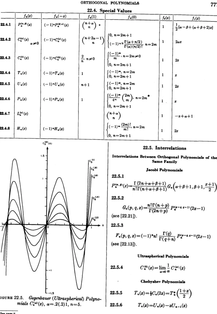
22.4. Special Values. ...

22.5. Interrelations ...

22.6. Differential Equations ...

22.7. Recurrence Relations ...

22.8. Differential Relations ...

22.9. Generating Functions ...

22.10. Integral Representations ...

22.11. Rodrigues’ Formula. ...

22.12. Sum Formulas ...

22.13. Integrals Involving Orthogonal Polynomials ...

22.14. Inequalities ...

22.15. Liiit Relations ...

22.16. Zeros ...

22.17. Orthogonal Polynomials of a Discrete Variable ...

Numerical Methods ...

22.18. Use and Extension of the Tables ...

22.19. Least Square Approximations ...

22.20. Economization of Series ...

References ...

Table 22.1. Coefficients for the Jacobi Polynomials Ppfl)(z) ...

n=0(1)6

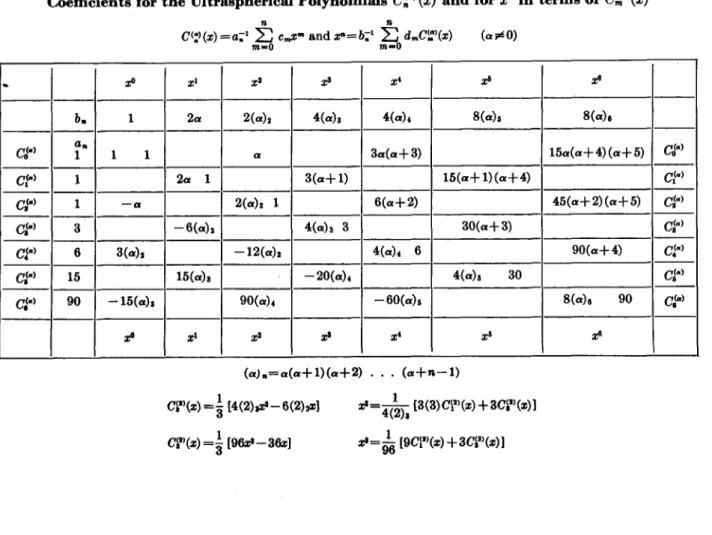
Table 22.2. Coefficients for the Ultraspherical Polynomials C’j? (5) and forz”inTermsof C:)(z). ...

n=0(1)6

Table 22.3. Coefficients for the Chebyshev Polynomials Z’,(z) and for s”inTermsof T&r) ...

n=0(1)12

Table 22.4. Values of the Chebyshev Polynomials T,(z) ...

n=0(1)12, ~=..(..)l. 10D

Table 22.5. Coefficients for the Chebyshev Polynomials U,(z) and for z”in Terms of U,,,(z) ...

n=0(1)12

Table 22.6. Values of-the Chebyshev Polynomials U,(z) ...

n=0(1)12, x=.2(.2)1, 10D

Page 773 773 774 775 777 777 781 782 783 783 784 785 785 785 786 787 787 788 788 788 790 791 792 793

794

795 795

796 796

* Guest Worker, Nationd Bureau of Standards, from The American University. (Pres- ently, Atomic Energy Commission, Switzerland.)

771

772

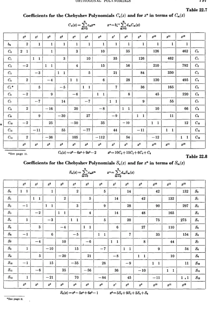
Table 22.7. Coefficients for the Chebyshev Polynomials C,(z) and for z”inTermsof Cm(z) . . . .

n=0(1)12

Table 22.8. Coefficients for the Chebyshev Polynomials S,(z) and for Z* in Terms of S,,,(z) . . . .

n=0(1)12

Table 22.9. Coefficients for the Legendre Polynomials P,(z) and for 9’

in Terms of P,(z) . . . . n=0(1)12

Table 22.10. Coefficients for the Laguerre Polynomials L,(z) and for 2”

in Terms of L,(z) . . . . T&=0(1)12

Table 22.11. Values of the Laguerre Polynomials L,(s) . . . . n=0(1)12, x=.5, 1, 3, 5, 10, Exact or 10D

Table 22.12. Coefficients for the Hex-mite Polynomials H,,(z) and for 2”

in Terms of H,(z) . . . . T&=0(1)12

Table 22.13. Values of the Hermite Polynomials H,,(z) . . . . n=0(1)12, x=.5, 1, 3, 5, 10, Exact or 11s

Page 797

797

798

799 800

801 802

22. Orthogonal Polynomials

Mathematical Properties 22.1. Definition of Orthogonal Polynomials

A system of polynomialsj,(x), degree [jn(x)]=n, is called orthogonal on the interval a<x_<b, with respect to the weight function w(x), if 22.1.1

s

b

w(~>$(~)j&)dx=0 a

(n#m;n, m=o, 1,2,. . .) The weight function w(x)[w(x) >O] determines the system j*(x) up to a constant factor in each polynomial. The specification of these factors is referred to as standardization. For suitably standardized orthogonal polynomials we set 22.1.2

s

b w(x)j~(x)dx=h,, jn(x)=k,x”+k:x~-‘+ ^{. . .}

@

(T&=0,1,2,. . ..) These polynomials satisfy a number of relation- ships of the same general form. The most important ones are:

Differential Equation 22.1.3 sz(x>f~+m(x>j~+~nfn=o

where gZ(x), m(x) are independent of 72 and a,, a constant depending only on n.

Recurrence Relation

22.1.4 .fn+‘=

where 22.1.5

Rodrigues’ Formula

22.1.6

$=L

d” I~(~N9(~~1”~

where g(x) is a polynomial in x independent of SZ.

The system consists again of orthogonal polynomials. - -

(1.5 P”(’

3

/ L

/=

\ 3 /

\

I-

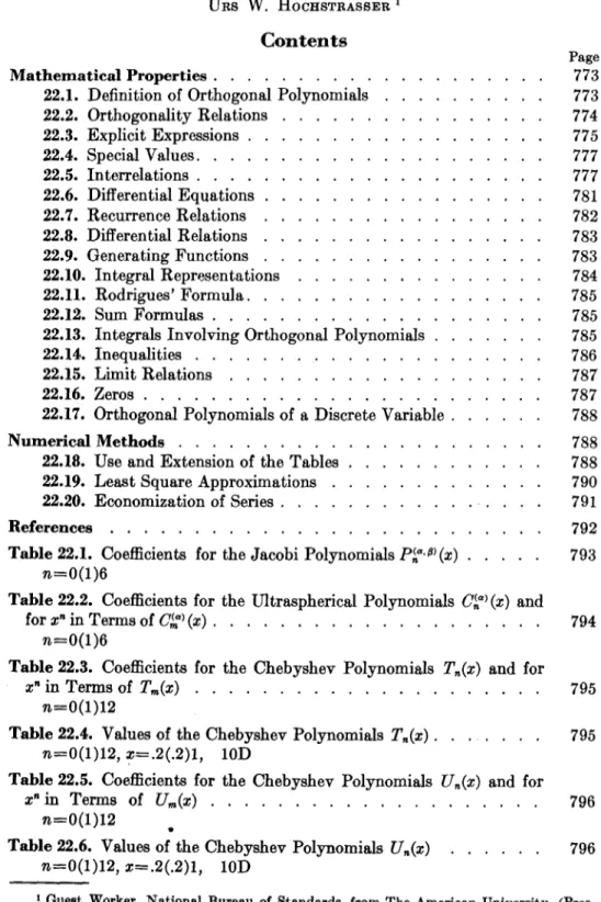
FIGURE 22.1. Jacobi Polynomials Pfi 8) (x) , a=1.5, /3=-.5, r&=1(1)5.

773

22.2.1 22.2.2 22.2.3

P$@ (2)

G.(P, q, 4 C”‘( I) = )

22.2.4

T&l

22.2.5

U” (4

22.2.6

cvd4

22.2.7

S.(z)

22.2.8

T: (4

22.2.9 22.2.10 22.2.11

f.(z) (ame of Polynomia a b w(z) Standardization h.

Jacobi Jacobi Ultraspherical

(Gegenbauer)

Chebyshev of the first kind Chebyshev of the

second kind Chebyshev of the

first kind Chebyshev of the

second kind Shifted Chebyshev

of the first kind Shifted Chebyshev

of the second kind

Legendre (Spherical) Shifted Legendre

-1 0 -1

-1

-1 -2 -2 0

0 -1

0 1 1 1

1

1 2 2 1

1

1 1

22.2. Orthogonality Relations

(l--2)*(1 +q (1 --2)D-a~a-1 (1--2*)a-t

(l---z’)-1

(1 --zqt

29 -4 (

>

( l-2 > + 4

(z--z’)-+ Tf(1) = 1

(x-x’)b

P$#‘(l)= n+a n ( >

k,=l C”‘(1) n

( n+2a-1

= n >

bf0)

T.(l) = 1

U,(l) =n+ 1 C,(2)=2 S,(z)=n+ ¹

q(1) =n+ 1 P.(l)=1

*+8+1 r(n+a+ l)r(n+B+ 1) 2n+a+o+1 n!r(n+a+8+ 1) n!r(fl+q)r(n+p)r(n+p-q+l)

(2n+~)r*Ch+~) w21-*r(n+2a)

n!(n+a)[r(41* a#0

1 2n+l

a=0

n#O n=O

n#O n=O

n#O n=O

*

= --

P

Remarks II>-1,8>-1 1-q> - 1, q>o a>--+

*See page 11.

22.2.13 L"(Z)

* 22.2.14 fin(Z)

* 22.2.15 He,(z)

--

22.3.1 22.3.2 22.3.3 22.3.4 22.3.5 22.3.6 22.3.7 22.3.8 22.3.9 22.3.10 22.3.11

-

-

Generalized Laguerre Laguerre Hermite Hermite

f”(Z) P’“. @) I (2) P-6) (J) ”

&(P, 4, d (72’ (2) cy (2)

T.(z)

Un(4 E-‘. (4 Lb) (2)

H.(z)

He.64

N n n n

[I ; [I

z

L-1 5

[I

z [I

;z

n

[I T

n L-1 5

-

-

22.2. Orthogonality Relations-Continued

0 m e-Q?

0 co e-*

--m co e-zz

k =(-1)”

n n!

k n -C--l)”

n!

e,=(-1)”

r(a+n+ 1) n!

1

&i2nn!

--a0 m ,-‘?t

e,=(-1)” &n!

22.3. Explicit Expressions f”w=d”mgc.h(z) d.

lYa+n+ 1) n!lYa+@+n+ 1)

r(q+n) r(p+W

n 3

n!

n!

("lfr") &) n r(a+8+n+m+l) 0 m . 2=r(a+m+l)

r(p+2n-m) (-‘)“, (3 r(q+n-m)

(-l)n rb+n-74 m!(n-2m)!

(-,)m (n-m-l)!

tn!(n-2m)!

(- l)m (n-m- I)!

m!(n-2m)!

t---11* (n-m)!

m!(n-2m)!

C---l)- (;,) (,,,,,) (--ljm (n"-';) ,$-

(--1)m '

m!(n-2m)!

(-- llm : m!2m(n-2m)!

Bn (4 (z- I)“-++ l)*

(x-l)“@

zm-m (22) “-*- (22) --*m (22) n-h (2x) n--l*

~“-*“I 2”

(2.z)"-+m Z"-*m

k.

1 2n+a+B 5 ( n >

1 (

2n+a+8 .jz n >

1 2" r(a+n) -arG)

2"

n n#O

2nd

2"

(2n) ! 2n(n!)*

(-l)n n!

2"

1

= --

-

Remarks a>--I,@>-1 a>-1, s>--1 P-q>-1, q>o a>-f> a#0 n#O, CA”(l)= 1

a>-1 ser! 22.11

a>-1

776

a4.0n

-X

FIQURE 22.2. Jacobi Polyrwmiata P!..@)(x), a=1(.2)2, 8=-J, n=5.

-I

FIQURE 22.3. Jacobi Polynomiala P>@(x), a=1.5, fl=-.8(.2)0, n=5.

Explicit Espressione Involving Trigonometric Function

f.(cose)=~ am COB (n--an@

m-0

fs(ms @I 0,

22.3.12

C”’ (CO8 I e) rbSm)r(a+n-m)

mun-m)![Iya)]’ a#0

22.3.13

P,(cos e) $ (“m”) (2:r:)

22.3.14

CiO) (c4x3 e> =i cos ne

22.3.15

T,(cos 8)=cos nB

22.3.16

U,(cos f3) = sin (n+l)e sine

FIQURE 22.4. Gegenbaw (Ultrmpherical) PO&W.+

mid C$)(x), a=.5, n=2(1)5.

ORTHOGONAL POLYNOMIALS

22.4.1

22.4.2

22.4.3

22.4.4 22.4.5

22.4.6

22.4.7

22.4.8

f”(Z) P$m (2)

C’“’ (2) I a#0

P’ (2) ”

T,(z) U.(z)

P” (4 Lp (2)

~I&)

f.(-4

(- l)“Pp(z)

(- l)q’(z)

(- l)“C~O’(Z)

(- l)“T.(z) t- l)nU”(z)

(- l)np”(z)

(- l)“H.(Z)

22.4. Z fvm ( >

n+a * n

(

n+2a- I

n

it n#O 2

1 n+l

1

L-l.5 22.5.5

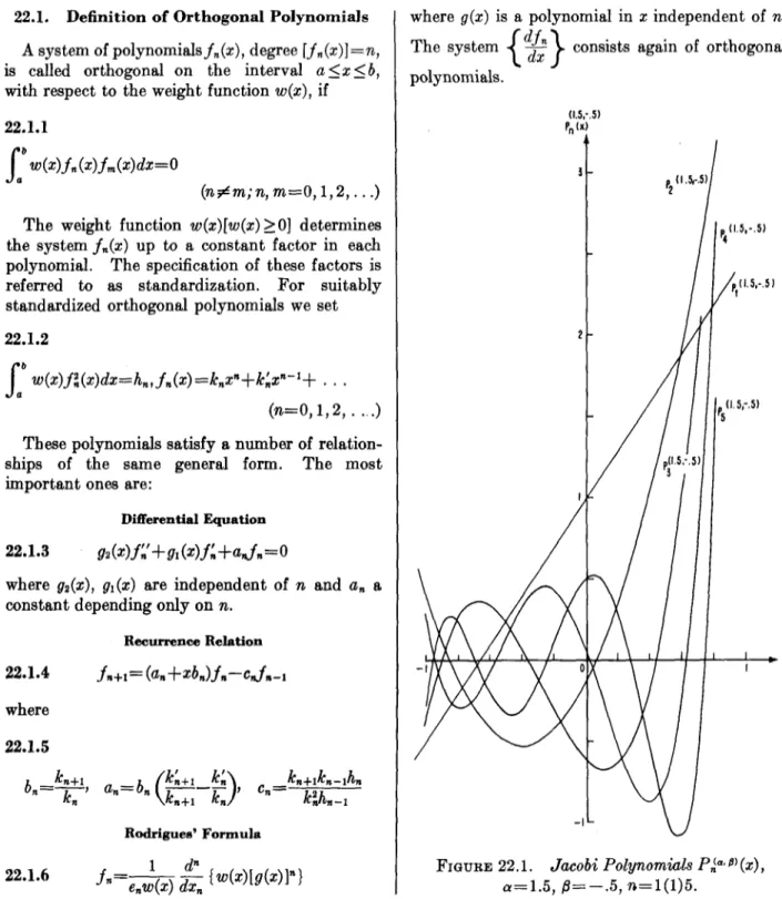
FIGURE 22.5. Gegenbauer (Uhasphmhzl) PO&LO- mials cy(z), a=.2(.2)1, n=5.

I i -

:cial Values f.(O)

10, n=2m+ 1 1

(- I)d* r(a+n’2), n=2m r(a) (n/2) !

I (-1)1

m 9 n=2m#O IO, n=2m+ 1

I (-l)m,

0, n=2m+ 1

1

(-1) m, ^n=%m 0, n=2m+ 1

:(-lin 2m , n=2m*

4”1 ( m >

.O, n=2m+l n+a ( n >

I (-1)” cm!

I

~8

(0, n=2m+l

-

-

fled

;[a--B+(a+Bf2)2]

2az

2x

2

2x

x

-x+a+ 1 2x

22.5. Interrelations

Interrelations Between Orthogonal Polynomials of the

Same Family Jacobi Polynomiab 22.5.1

ppyz>= r b+a+b+l)

nW+a+B+l) G. a+B+l,B+l,T)

(

22.5.2

Q*(p, *,+n!r(n+p) ~y*--1y22-1) r(2n+P)

(see [22.21]).

22.5.3

F,(p, q,z)=(-l)“n! = P;~-~*Q-“(2r-l) r(n+n>

(see [22.13]).

Ultraspherical Polynomials

22.5.4 c:‘(z)=lim; cp’(z)

Chebyshev Polynomiab

22.5.6 T”(z)=u”(z)--zu”-l(4

778

22.5.8

T&)=3 [u,(z)-u”-2(4l

22.5.9 u.(r)=s.(2it)=u:(~)

22.5.10 U.-I(X)=~-~

J- [z~“(z)--*+1(41

22.5.11 C,(z)= 2T” (;)=2 T*, (y) 22.5.12 c”(x>=&(z~--s,-*~~~

22.5.13 s.(x)=u.(;)=u:(q

22.5.14 2’*,(s)=2’,(22-1)=3 C,,(4z-2) (see [22.22]).

22.5.15 U~(cc)=5.(4~-2)=U,(2z--) (see [22.22]).

Generalized Laguerre Polynomials

22.5.16 Ltp’(x)=L,(x)

22.5.17

Lph)=(-l)m gm [L+mb$l

Hermite Polynomials

22.5.18 He,(x)=2-“‘*H, z

0 4 (see [22.201).

22.5.19 H,(~)=2~l*Ele.(xJZ) (see [22.13], [22.20]).

Interrelations Between Orthogonal Polynomials of

Difllerent Families

22.5.20

Jacobi Polynomials

22.5.21

22.5.22

12.5.23

PA--‘* -*) (x) =& (F) T,(x)

12.5.24 i2.5.25

P!“*O)(x)=P,(x)

Ultraspherical Polynomials

7:“,‘(x)= r(a+Qb!2**

r(a)(2n)! Pp-,) (22*-l) 22.5.26

(am

WO)

12.5.27

22.5.28

(a#O)

Cbebyshev Polynomials

22.5.29 T,.+,(z)=& zPk-“t’(2~2--1) n!fi

22.5.30 U*n(“)=r(n++) p$ -1, (2&- 1) 22.5.31 T”(@=r(n+4j 2!!@- pc-t. 4) @) z 22.5.32 ua(2)=2r(n+*) ^(n+l)!fi Pi** 1) (x)

FUXJRE 22.6. Chebyshev Polynomials T*(X),

%=1(l)&

*See page xx.

ORTHOGONAL POLYNOMIALS

779

I2 -

I2 -

FIWRE 22.7.

FIWRE 22.7. Ciieby~hu Polynomials Ciieby~hu Polynomials U,(x), U,(x), T&=1(1)5.

T&=1(1)5.

22.5.33

22.5.33

T.(x) T.(x) =; CkO) =; CkO) (2) (2)

22.5.34

22.5.34

U,(x>=C~‘)(x) U,(x>=C~‘)(x)

Legendre Polynomials

22.5.35 P.(x)=P$yz) 22.5.36 P, (5) = cy) (z) 22.5.37

g [P&)1=1.3 . . . (2m-l)C$!!_+,+)(z) Cm 234

Generalized Laguerre Polynomials

22.5.38

22.5.39 W”‘(x) =?&&j ^JJ2.+1(da

Hermite Polynomials

22.540 Ha,(z) = (- 1)m2”m!L$1/2) (z2) 22.5.41 H2,+,(5)= (-l)‘“2k+1m!zLg’2)(z2)

Orthogonal Polynomials as Hypergeometric Functions (see chapter 15)

fn(x>=@(a, 6; c; dx))

For each of the listed polynomials there are numerous other representations in terms of hyper- geometric functions.

22.5.42 22.5.43

22.5.44 22.5.45

22.5.46

22.5.47 22.5.43 22.5.49

22.5.50 22.5.51 22.5.52 22.5.53

f. (2) Py(x) P$8'(2) P$"(x) P'.".@(z) C"' (x) $8 T.(x) U.(x) P,(x) P"(X) P,(z) Pdx)

%+I(4

d

Un+2a)

n!l-(2a)

1 n+l

n CW!

(- 1) 22qny (- 1)“(2n+ 111

-2qGpZ

a

l .

-n

-n --A -n -n -n -n -n -n -- n

2

-n

-n

b n+cr+Is+l -n--o!

--n-B -n-a n+2a n

n+2 *

n+l --n

l-n

2 n+&

n+t

C

r+1

-2n--a--8 a+1 8+1 a++

f

% 1 -2n i-n 4 9

VW 1-Z -3-

2 1--2 x-l z+i x+1 z-i

l-2 -T

l-2 -3-

l-2 2

l-x 2

2 1--z

1 2 29 39

780

Functions (see chapter 13)

22.5.54 L:a’(x)=~;a)M(-n, a+l, r)

Orthogonal Polynomials as Parabolic Cylinder Functions (see chapter 19)

22.5.55 H, (5) =2”U

( ;-; n, ;, x2

>

22.5.56 H,,(z)=(-l)-@$M(-m,;rzz) 22.5.57

(2m+l)!

* Hzm+l(~)=(--l)~ m! 2xM(-m, iJ x2)

P”(X)

I

FIGURE 22.8. Legendre Polynomials P,(x) ,

n=2(1)5.

‘OLYNOMIALS

22.5.58

H,(x) =2*~2ez2/2D,,(JZx)=2n~2ez2/2U 22.5.59 He,(x)-ee’2/4D,(x)=e”2/4U

Orthogonal Polynomials as Legendre Functions (see chapter 8)

22.5.60 cp (2) =

r(a+i>r(2cY+n) 1

n!Iy242) [z (22-q-~ P$q$, (5)

FIGURE 22.9. Lagumre Polynomials L,,(x), n=2(1)5.

FIGURE 22.10. H&9

Hermite Polynomials 7) n=2(1)5.

ORTHOGONAL POLYNOMIALS 22.6. Differential Equations

g2(2)y”+g1(x)y’+go(x)y=o

781

22.6.1 22.6.2

22.6.3

22.6.4

22.6.5 22.6.6 22.6.7 22.6.8 22.6.9 22.6.10 22.6.11 22.6.12 22.6.13 22.6.14 22.6.15 22.6.16 22.6.17 22.6.18 22.6.19 22.6.20 22.6.21

Y P$@ (2)

(1 --z)“(l +z)~P(*~~)(.z) n -+I 8&l (1 --z);;-(1 Sz) * fy’(2)

(,i” g+ycos ,y++ Py (cos 2)

C”‘( ) I =

(1 -zpc(q n x ) (,-~*)~+~ Cc,)(x)

(sin r)%$“‘(cos x) Tdr)

T,(cost) - T"(Z) ; ^v,-lb) lJ.(z)

Pm(x) 4i=3P.(z) L;'(z)

*

e-rxa’2L~Q) (5) e-z12z(atI)12q4 (r)

*

,-**/2,“+4L’,“’ (x’)

H.(z) 2 e-yH,(s) He.(x)

sdz) l-22 1-x*

1

1

1-Z l--22

1

1 1-9 1 l-22 l-22 1-Z 1 x 1;

1

1 1 1 1

_-

I

I

-

-- __-.--- 91(z) 8-a-((2+B+2).r a-P+(a+B-2)x

D

D

- (2,-l- I)2 (2a - 3)x 0 0 -X 0 -3x -3x -2%

0 a+1--2

&+I

0 0 -2.z 0 -X

n(nta+P+ 1)

n(n+2a)

n*

n*

n*- 1 n(n+2) n(n+ 1) n(n+ 1)

l-xl +(Lxy*

n n+;+1-g

2n+a+i+1--(r2 1

___ __--

2x 4x2 4

1--a*

4n+2a+3-x*+7 2n 2n+ 1 -x1

n

782

22.7.1

fn

22.7.2 Gnh q, 2)

22.7.3 22.7.4 22.7.5 22.7.6 22.7.7 22.7.8 22.7.9 22.7.10 22.7.11 22.7.12 22.7.13 22.7.14

Cl”‘(x) T,(x) U,(x) S”(X) cm T.’ (4 Kc4 p. (4 p:(x) L!“‘(x) He64 He,(z) -

ORTHOGONAL POLYNOMIALS

22.7. Recurrence Relations

Recurrence Relations With Respect to the Degree n

al,fn+l(x)= (aan+aanr)fn(x) -a4,fn-l(Z)

aIn

n+1 1 1 1 1 1 1 n+l n+l n+l 1 1

ah

-[2n(n+p)+q(p-11))

(2n+p72)3 0

0 0 0 0 -2 -2 0 -2n-1 2n+(u+1 0 0

--

-

Miscellaneous Recurrence Relations Jacobi Polynomials

22.7.15

( ^n+g+i+1) (l-z)P~+‘+~)(z)

= (n+a+ l)P,‘a*@ (2) - (n+ l>P’&B, (z) 22.7.16

(

n+E+-+1 B (l+z)PpJ+l)(,) 2 2 >

=(n+B+I)P~s)(2>+(n+l)P~~Pi)(~) 22.7.17

(l--)P~+‘,s)(2)+(1+2)P%‘8+1’(2)=2P~8)(s) 22.7.18

(2n+cu+B)P~-',8'(2)=(n+(y+B)P~,8'(~)

-(n+Bv%P(~)

22.7.19

(2n+a+P)P~,8-"(2)=(n+a!+B)P~,8'(s)

+ (n+cY>PgyJ(az)

22.7.20 Plp,S-l)(,)-P~-l.S)(,)=P~~)(z)

ah

@n+a+Bh (2n+p-2)4

@n-!-p-l) W+ff) 2 2 1 1 4 4 2n+l 4n+2 -1 2 1

ah

2(n+a)b+i3)

Ghfa+B+2) n(n+r-l)b+p-1)

(n+P-dm+P+l) n+2n-1 1 1 1 1 1 1 n n n+a 2n n

Ultraspherical Polynomials

22.7.21

2~(1--;c2)C~_:“(2)=(2a+n--)C~,(2)--n2C~’(z) 22.7.22

=(n+2cY)zC~'(z)

-(n+lm%(~)

22.7.23 (n+(~)C~~~‘(2)=(ru-l)[c~:1(5)-C~l(~)]

Chehyshev Polynomials

22.7.24

2 T,(z) T&l = T?l+m (z) + ~,-I&$ (n>m> * 22.7.25

2(sc2-1)um-~(2)un-1(5)=T,+,(s)--T,_,(s)

(n2 m>

22.7.26

2T,(2)Un-1(2)=Un+,-1(2>+Un-m-*(2) 22.7.27

2T,(z)U,-,(s)=U,+,-l(s)--u,-,-*(2) 22.7.28 2T,(z)U,-,(5)=Uz,-l(z)

*See page II.

(n>m)

(n>m)

ORTHOGONAL POLYNOMIAL& 783

General&d Laguerre Polynomials 22.7.31

22.7.29 Lp+yz)=~ [(72+Ly+l)L~)(2)-((12+l)L~,(2)]

Lp+yI)==; [(z--n)L~“‘(z)+(ar+n)Ljp_‘,(z)] 22.7.32

22.7.30 L~-')(~)=L,='(z)--L~*(z) Q-')(z)= &a [(nt-l)~~1(2)-(nSl--z)L~'(z)l

22.8.1 Pp’ (2)

22.8.2 c!=) (2)

22.8.3 T&)

22.8.4 U.(z)

22.8.5 PA4

22.8.6 L!“) (2) 22.8.7 HI&)

22.8.8 He,@)

f&)

-- 22.9.1 22.9.2 22.9.3 22.9.4 22.9.5 22.9.6 22.9.7 22.9.8

P$fl(x) cp (2) cp (2) c#y (2) C” (2) I T,(z) T&J

‘J”.W

22.9.9 22.9.10 22.9.11

*see page n.

f.

22.8. Ihfferential Relations Ql(z)~f.(z)=g*(z)f"(z)+no(z)f"-~(~)

61 (zn+a+B)(l-z*) 1-Z’

1-X’

l-9 1-Z’

2 1 1

B1 7&-B- (2n+a+BM

--Rz * -nx -7l.l -TIX n 0 0 22.9. Generating Functions

1 NW rb+t)rcb+4

2 42 2n Gn _{( >}

1 n 1 1

42 2n+2 pi ( n+1 >

R= Jl-2zz+z2

-

go

v

2(n+a)b+f9) n+2a-1 n n+l n - (n+a) 2n n

g(w) Remarks

R-‘(l--e+R)-“(l+e+R)-8

R-h --In R’

eam*~(;sin*)L-al.-t(asinB) (9+1)

R-‘(l--ZL+ R)*fi 1-4 In R*

l-22 R’

R-1

$ (1--zz+R)-“2 *

Id<1 bl<l,aZO bl<l,afO bl<l x=cos 9

--1<2<1 l4<1 -l<:<l

Id<1 ao= I

-l<z<l IKl -l<x<l

l4<1 - l<z<l

14<1 -l<z<l

Id<1

784

22.9.12 22.9.13 22.9.14 22.b.15 22.9.16 22.9.17 22.9.18 22.9.19

22.10.1 22.10.2

b 22.10.3

22.10.4 22.10.5 22.10.6 22.10.7 22.10.8 22.10.9

A(4 P*(z) P”(4 u4 L”’ (2) I) LA=’ (4 H,(z) Hd4 Han+* (4

ORTHOGONAL POLYNOMIALS

22.9. Generating Functions-Continued

/I A

1 1 J 1 1

1 *

IYnSa+l) 1 ii (-.I)”

(2n) ! C-1)”

(2n+ l)!

4 g@, 4 Remarks

R-1 /J

e* 0”’ ‘J&e sin 0) (l-zz+z’)-’

(l--r)-*+ exp (5) (x~)-t~e~~.(2(xz)*~~l elZ,-”

ez co9 (226) * rl’*e* sin (2~4) t 22.10. Integral Representations

Contour Integral Representationa

-l<z<l IKl z=cos 6

-2<2<2 Id<1 M<l

2 ( t, z)ds where C is a closed contour taken around z=a in the positive sense f&J)

Tdz) U.(x) Pm Pm Lyx) I L,$qz) H,(z)

BOW

(1 -x)$1 +2p

1

112 1 1 1 5 e97 1

?Z!

Bl (64

21-l 2(2-x) l/z

l/t

21-l I-2

e E-2

1+;

l/S

gdwz) (1 - E)‘(l+ z)@

2-X (1--22~+z’)-9-’

1 - 2’

e(l-2Zz+E’) 1 2(1-222+r*) i (l-Ls+e’)-“~

- 1 Z-2 - ,“, e-’

e-* ( 1+: > Y/z

esz*-rl 2

a Remarks

f 1 outside C Both zeros of

1 - 2zr+ a’outside C, a>0

Both zeros of I-2zz+z*outaideC Both zeros of

1 - 22~ + z* outside C Both zeros of

1 - 2zc+ ES outside C

Zero outside C z= --z outside C

Miacdaneoue Integral Representations

(a>O)

ORTHOGONAL

22.10.12 P,(cos e) =-;

s * (cos O+i sin e co9 fp)U#~

0

22 10 13 P,(cos e,d . . * sin (n+wJd4

* n- s 0 (co9 e-cos +)*

POLYNOMIALS

785

22.10~14 ~g)(x)=$ m e-It”+; J,@&)dt .s ⁰

22.10.15

H,(x)=e’* T srn e-l*t” cos (2&-i,) dt 0

22.11. Rodrigues’ Formula

The polynomials given in the following table are the only orthogonal polynomials which satisfy this formula.

I

22.11.1 PFp 8) (2) (- 1)“2%!

22.11.2 cp (2)

(- 1)“2”n!

rcwr(a+n+3)

;{;,+I r(n+2a)

22.11.3 T&J f

(-1)“2” 1/;; *

22.11.4 Us&) x*i

Pd4

y;;;, (fi:“:,%

. . L?‘(x) n!

22.11.7 H,(z)

22.11.8 He,(z) [I:{” II

(1 --z)“(l +iry (l-@a-t (1 -cl?)-’

(l-21)’

1 e-97 p’

&2

d4 1-Z’

1-Z 1-Z’

1-Z l-24 2

;

22.12.1

22.12. Sum Formulas Christoffel-Darboux Formula

Miscellaneous Sum Formulas (Only a Limited Selection Is Given Here.)

22.12.2 Q2&~=t[l+u*n(41

22.12.3 _g; ~*m+1(4=3U*n-1(5) I

Tl

22.12.4 isou2"(4' ^l-T*n+2(4 2(1-x*) 22.12.5

22.12.6 ~oLl’(x)~~~~(y)=L~+B’.‘(z+y)

22.12.8

22.13. Integrals Involving Orthogonal Poly- nomials

22.13.1

2n ‘(l--y)“(l+y)Bp:“,8)(y)dy s

~~lp_~‘,B+l’(~)-(~~x~~+l(l+x~~+lp~~~l~~+l~~~~

22.13.2

=cyp(O)- (l-2yqy(2!) 22.13.3 r’ Tn Mdy

JTl (y-x)~=Tu~-l(x)

_cl vT=i%&)dy =-nTn,xl

22.13.4 - *

J-I (Y--X)

22.13.5 s

’ (1-x )-l/*P.(x)dx=& *

-1

22.13.6

s 0 * Pz.(cos @de=& p>’

22.13.7

S

- . ,

*See page Ii.

786

22.13.8 22.14. Inequalities

22.14.1

22.13.9

CA>-2) 22.13.10

s

“P,odt= 1

-1 &3 (n+i)fi [T&l +Tn+l(41 22.13.11

S 2 q=q-(n+a;Fx l P,(t)dt [~n(x)--n+1(91

22.13.12

s zm e-*Lr)(t)dt=e-“[L~‘(X)-L$)P-‘1(2)]

22.13.13

r(a+p+n+l)Joz (x-t)@-+LP)(t)dt

=r(cu+n+i)r(~))+BLP+B)(2) (A%%>--1, m>w 22.13.14

s = Lm(t)Ln(x-t)dt

0

S

= L,+,(t)dt=L,+“(x)---L,+“+l(x)

0

22.13.15

S

0

22.13.16

S

0

S

22.13.17

0)

-m e-f2H2,(tx)dt=fi y (9-l)”

22.13.18

S -m m e-f2tH2,+l(tx)dt=~ Pm+l)! mr x(x2~l)m

22.13.19

/rm

J-m

22.13.20

S me-r2[H,(t)]2

i

( >

Ic?~)(x)I 5 b+--l,8>-1)

IP$e)(z’)I -$t if *<--l 2’ maximum point nearest to -

8-a

a+P+l 22.14.2

la%M {

(“‘y> (a>01 Ia@W>l (-f<a<o)

x’=O if n=2m; x’=maximum point nearest zero if n=‘2m+l

22.14.3

~W(cos @1<2’-= (sinne;‘;(a) (O<(ll<l, o<e<4 22.14.4

IT&)ll1

22.14.5 dTn (4 I - I ^<n2

dx (-11x11)

22.14.6 IUn(x)l In+1 (-l<z<l) 22.14.1

IPn (4 I I 1

I ----&-- I Ip(n+l) (-l~s~l) 22.14.9 IPn(x)l 2

J 2 --i-

7m4&? (---l<dl) 22.14.10

~‘.o-P~-l(,)P~+l(x)<3~n~l)

22.14.11

1 -P’,(x)

Pn2(x)-PAdPn+1(x~2 (2n-l)(n+1)

(-l<x<l) 22.14.12

ILd4 I I fP (x2 0)

22.14.13 1 Lp) (x) I 5 LfrTr:.:) ezj2 620, x20) 22.14.14

ORTHOGONAL POLYNOMIALS 787 22.14.15 I&,(z) 15 ez2’222nr~! 22.15.2 fi [; L:) (;)]=r-a/v,(2&

22.14.16 22.14.17

22.15.1

(x20> 22.15.3 lim W,“dEH r

n+m 4”n! In zfi

HI

n-t- 4%!

22.15. Limit Relations 22.15.5 =LP’ (2)

22.16. Zeros

For tables of the zeros and associated weight factors necessary for the Gaussian-type quadrature formulas see chapter 25. All the zeros of the orthogonal polynomials are real, simple and located in the interior of the interval of orthogonality.

Notations:

Explicit and Asymptotic Formulas and Inequalities

xg)mth zero of fn(x) (xj”)<xP< . . . <x?)) e:)=arccos ~$~+~(o<ejn)<ep< . . . -0X4

j, %, mth positive zero of the Bessel function Jol(x) O<j, l<ja,2< . - .

22.16.1 22.16.2 22.16.3 22.16.4

Py)(cos e) C’“‘( n x ) C’“’ (co9 I?) n

T&) 22.16.5 U.(x)

22.16.6 P,(cos e)

22.16.7 P.(x)

22.16.8 L’“’ (2) II

f”(Z)

= --

Relation lim nf$?=j,,, &>-I, s>-1)

Ta+-

&pcos 2m--1 *

2n xg)=cos 2% *

n+l

i

2m-1

- r<ti”‘< 2m 2n+l -“-2n+lR

4m-1 1

e(p=- 4m- 1

4n+2 “+8n’ Cot 4n+2 - r+O(n-y

+()(+)

k,=T+q

For error estimates see [22.6].

788

22.17. Orthogonal Polynomials of a Discrete Tw*(xi) is finite. The constant factor which is Variable

still free in each polynomial when only the orthogo- In this section some polynomialsf,(x) are listed nality condition is given is defined here by the which are orthogonal with respect to the scalar explicit representation (which corresponds to the

product Rodrigues’ formula)

22.17.1 KJm’=~ w*(xtYn(x*)f,(xi>. 22.17.2 fn(x)=--&

n A”[w*(xMx, n)l

The xi are the integers in the interval a<x& b where g(x, n)=g(x)g(x-1) . . . g(x-n+l) and and 20*(x<) is a positive function such that g(x) is a polynomial in x independent of n.

Name

Chebyshev Krawtchouk Charlier Meixner Hahn

= --

-

- a

= --

-

b

N-l 1

N OD 03 0)

p-J”-= x 0 e-au=

x!

c=r(b+x) r(b)x!

r(b)r(c+z)r(d+z) s!r(b+x)r(c)r(d)

=

-- ^w*(x)

= --

-

l/n!

(- l)nn!

(-l)ndann!

C”

n!

= _-

-

dx, 4

(3 (“n”>

qv!

(x-n)!

x!

(z-n)!

X!

(x-n)!

x!r(b+x)

(x-n)!r(b+z-n)

= _-

-

Remarks

P, q>o;

p+q=l a>0 b>O, O<c<l

For a more complete list of the properties of these polynomials see [22.5] and [22.17].

Numerical Methods

22.18. Use and Extension of the Tables

Evaluation of an orthogonal polynomial for which the coe&ients are given numerically.

Example 1. Evaluate La(1.5) and its first and second derivative using Table 22.10 and the Horner scheme.

I 2=1.5

1 1.5

1 1.5

1

-36 450 - 2400 5400 - 4320

1. 5 -51.75 597.375 - 2703. 9375 4044.09375

-34.5 398. 25 - 1802. 625 2696.0625 - 275.90625

1. 5

733.0 1. 5

-31.5

-49.5 523. 125 - 1919. 25 1165. 21875 L -306. 140625

6- 720

348. 75 - 1279. 500 776. 8125 889. 3125

-47. 25 452. 250 - 1240. 875

301. 50 -827. 250 - 464.0625

-

=

- -

-

720 - 413. 859375

306. 140625

=. 42519 53

L,=889. 3125

6 720

= 1.23515 625 L,,=2 [ - 464.06251

(I 720

=-I. 28906 25

ORTHOGONAL POLYNOMIALS

789

Evaluation of an orthogonal polynomial using the explicit representation when the coe&ients are not given numerically.

If an isolated value of the orthogonal polynomial f*(x) is to be computed, use the proper explicit expression rewritten in the form

fkd =&(4dx~

and generate a,,(r) recursively, where

a,-l(x)==l -~jCW.Cx) (m=n, n-l, . . ., 2, 1, a,(z)=l).

The d,(x), b,, c,,.f(z) for the polynomials of this chapter are listed in the following table:

fn(4

p’u, 8) ” cl”,’

C’“’

an+1

T an T 2?I+1 u In u 2”fl Pl, P a*+1 Lb’ n

Hzn H ail+1

- I

dn(4 ( n+a >

(-n. $?

(-1)” kp .,&

C-1)”

(-1)n(2n+1)2 (-1)”

(-1)“2(n+l)z!

(-1)” 2n

-( 4” n >

0” %+I

(n+l)x

4” ( n >

(-1)” @n+l)‘&

n!

bm

(n-m+l)(a+B+n+m)

Z(n-m+l)(a+n+m-1) P(n-m+l)(a+n+m) Z(n--m+l)(n+m-1) 2(n-m+l)(n-tm) 2(n-m+l)(n+m) 2(n-m+l)(n+m+l) (n-m+1)(2n+2m-l) (n-m+1)(2n+-2m+l) n-m+1

2(n-m+ 1)

2(n-m+ 1)

= I

2m(a+m) m(2m- 1) m(2m+ 1) m(2m- 1)

m(2m+ ¹⁾

m(2m- 1) m(2m+ 1) m(2m- 1) m(2mS 1) m(a+m) m(2m- 1)

m@m+ 1)

Example 2. Compute Z’~1’2*3i2)(2). Here de= =3.33847, f(2)=-1.

m 8 7 6 5 4 3 2 1 0

i: 1 1. 132353 1.366667 48 1.841026 60 3.008392 70 6.849651 78 26.44156 84 223. 1091 88 6545. 533 90

%I 1;: 1:: 78 55 36 21 10 3 0

~~*‘2~3’2’(2)=d~,(2)=(3.33847)(6545.533)=21852.07

Evaluation of orthogonal polynomials by means of their recurrence relations Example3. Compute@)(2.5)for n=2,3,4,5,6.

From Table 22.2 C$)= 1, C?= 1.25 and from 22.7 the recurrence relation is

n 2 3 4 5 6

-___

cq2 n * 5) 3. 65625 13.08594 50.87648 207.0649 867.7516

Check: Compute @‘(2.5) by the method of Example 2.

790

In some applications it is more convenient to use polynomials orthogonal on the interval [0, 11.

One can obtain the new polynomials from the ones given in this chapter by the substitution x=2:- 1.

The coefficients of the new polynomial can be computed from the old by the following recursive scheme, provided the standardization is not changed. If

“f”(X) =gowm, f:(z)=~~(2z-l)=~~u~zm then the n: are given recursively by the a,,, through the relations u~)-~u~-~‘-u~~,; 7n=n-1, n-2, . . ., j; j=O, 1, 2, . . ., n am (-‘)=a,/2, m=O, 1, 2, . . ., n

u$)=2&,j=O, 1, 2, . . ., n and u~~,“‘=uZ; m=O, 1, 2, . . ., n.

Example 4. Given Ts(z)=5z-20z3+16z5, find T:(z).

‘m 5

\

4 3 2 1 0

j

-1 f+ &” 0 -lo=&-” 0 2.5=a;-*) 0

0

1 it

-16 -4

-64

3;:

-4: 5L;

-1=a;

P 1;:

- 192 -4oo=a;

-512 1120=a;

t

256 - 1280=a;

512=a;

Hence, Z’,*(z)=512xs-1280x4+1120z3-400x2+50x---1.

22.19. Least Square Approximations

WMf(4!JW~

if D is a continuous interval

Then

if D is a set of N discrete points x ,,,.

where

*

am= (j, jmMj~9 &de

*f(z) haa to be square integrable, see e.g. ^(22.17).

Problem: Given a function j(z) (analytically or in form of a table) in a domain D (which may be a continuous interval or a set of discrete p~ints).~

Approximate J(Z) by a polynomial F,,(z) of given degree n such that a weighted sum of the squares of the errors in lJ is least.

Solution: Let w(z) 20 be the weight function chosen according to the relative importance of the errors in different parts of D. Let j,,,(x) be orthogonal polynomials in D relative to w(z), i.e.

Cj,,,, j,,) =0 for m #n, where

D a Continuous Interval

Example 5. Find a least square polynomial of degree 5 for j(z)=kx J in the interval 21x15, using the weight function

1 W(Z)=,&x-2)(5-x)

which stresses the importance of the errors at the ends of the interval.

Reduction to interval [-1, 11, t=2q

w(x(t)> 2 1

3 Jl-t2 From 22.2, jm(t) = Z’,,,(t) and

4’1 1

um=3?r

S

2 l 1

di!

u”=3?, s -, Jiq t+3 --

*See page II.

OR!l’HOGONAL POLYNOMIAL& ₇₉₁

Evaluating the integrals numerically we get --.235703-.080880Tl 1

1+x + .013876Tz (F)- .00238OT, rq)

D a Set of Discrete Points

If x,,,=m(m=O, 1, 2, . . ., N) and w(x)=l, use the Chebyshev polynomials in the discrete range 22.17. It is convenient to introduce here a slightly different standardisation such that

Recurrence relation: jO(x) = 1 ,ji(2) = 1 -g

(n+l>(N-~)j”+l(~)=(2~+1)(~--x)j”(~)--n(~+~+l)j~-l(x)

Example 6. Approximate in the least square sense the function j(x) given in the following table by a third degree polynomial.

2 I

I

10 .3162 0

:: : 2673 2887 1

:

:: : 2357 2500 i : 1

1,; -1,; 4

-l/1 -7); $

-1 1 -1

hcf) fl (3 j*m f2m

5

1.3579 .09985 .01525 .0031

(f t fn>

an=(fn, .271580 .039940 .0043571 .000310

j(x)-.27158+.03994(3.5-.25x)+.0043571(23.5-3.5x+.125;Ga)+.00031(266-59.8333x

j(x) +.59447- .043658x+ .00190092- 9000322921 +4.375x2-.10417x33)

22.20. lkonomization of Series 1 Then, since IT,(s)l11(-l<x<l) Problem: Given j(x)= 2 a,x’ in the interval

m=O

-11x11 and R>O. Findy(x)=g b,,,xmwith N m=O

as small as possible, such that /y(x)-j(x) I<R.

Solution: Express j(x) in terms of Chebyshev polynomials using Table 22.3,

-j(x) =m.fo b, T,,, (x) within the desired accuracy if

I% lbml<R

w-N+1

f(x) =m$o bm T,(x)

792

R=.05.

From Table 22.3

.I(~)=~~~149~e(z)+32~~(~)+3~,(~)1

&I=&, W’o(4+32Tz(41+& F’6~1(~)+11~d~~l

+~[76~~(~)+llT,(z)+~~(~)l ^since

References

Texts

[22.1] Bibliography on orthogonal polynomials, Bull. of the National Research Council No. 103, Wash- ington, D.C. (1940).

[22,2] P. L. Chebyshev, Sur l’interpolation. Oeuvres, vol. 2, pp. 59-68.

[22.3] R. Courant and D. Hilbert, Methods of mathe- matical physics, vol. 1, ch. 7 (Interscience Publishers, New York, N.Y., 1953).

[22.4] G. Doetsch, Die in der Statistik seltener Ereignisse auftretenden Charlierschen Polynome und eine damit zusammenhiingende Differential- differenzengleichung, Math. Ann. 109, 257-266 (1934).

[22.5] A. ErdBlyi et al., Higher transcendental functions, vol. 2, ch. 10 (McGraw-Hill Book Co., Inc., New York, N.Y., 1953).

[22.6] L. Gatteschi, Limitazione degli errori nelle formule asintotiche per le funzioni speciali, Rend. Sem.

Mat. Univ. Torina 16,83-94 (1956-57).

[22.7] T. L. Geronimus, Teorla ortogonalnikh mnogo- chlenov (Moscow, U.S.S.R., 1950).

[22.8] W. Hahn, tuber Grthogonalpolynome, die q- Differenzengleichungen gentigen, Math. Nachr.

2, 4-34 (1949).

[22.9] St. Kaozmarz and H. Steinhaus, Theorie der Orthogonalreihen, ch. 4 (Chelsea Publishing Co., New York, N.Y., 1951).

[22.10] M. Krawtchouk, Sur une g6nt%lisation des poly- nomes d’Hermite, C.R. Aced. Sci. Paris 187, 620-622 (1929).

[22.11] C. Lanczos, Trigonometric interpolation of empir- ical and analytical functions, J. Math. Phys.

17, 123-199 (1938).

[22.12] C. Lanczos, Applied analysis (Prentice-Hall, Inc., Englewood Cliffs, N.J., 1956).

[22.13] W. Magnus and F. Oberhettinger, Formeln und Siitze fiir die speziellen Funktionen der mathe- mat&hen Physik, ch. 5, 2d ed. (Springer- Verlag, Berlin, Germany, 1948).

[22.14] J. Meixner, Orthogonale Polynomeysteme mit einer besonderen Gestalt der erzeugenden Funk- tion, J. London Math. Sot. 9, 6-13 (1934).

[22.15] G. Sansone, Orthogonal functions, Pure and Applied Mathematics, vol. IX (Interscience Publishers, New York, N.Y., 1959).

[22.16] J. Shohat, ThQrie g&&ale des polynomes ortho- gonaux de Tchebichef, MBm. Sot. Math. 66 (Gauthier-Villars, Paris, France, 1934).

[22.17] G. Szego, Orthogonal polynomials, Amer. Math.

Sot. Colloquium Publications 23, rev. ed. (1959).

122.181 F. G. Tricomi, Vorlesungen tiber Orthogonalreihen, chs. 4, 5, 6 (Springer-Verlag, Berlin, Germany, 1955).

Tables

[22.19] British Association for the Advancement of Science, Legendre Polynomials, Mathematical Tables, Part vol. A (Cambridge Univ. Press, Cambridge, England, 1946). P,(z), 2=0(.01)6, n=1(1)12, 7-8D.

[22.20] N. R. Jorgensen, Undersbgelser over frekvens- flader og korrelation (Busck, Copenhagen, Den- mark, 1916). He,(z), 2=0(.01)4, n=1(1)6, exact.

[22.21] L. N. Karmazina, Tablitsy polinomov Jacobi (Izdat. Akad. Nauk SSSR., Moscow, U.S.S.R., 1954). C.(p, q, z), z=O(.Ol)l, q=.l(.l)l,

p=1.1(.1)3, n=1(1)5, 7D.

[22.22] National Bureau of Standards, Tables of Cheby- shev polynomials S.(Z) and C,,(r), Applied

Math. Series 9 (U.S. Government Printing Office, Washington, D.C., 1952). 2=0(.001)2, n=2(1)12, 12D; Coeflicients for T.(Z), U,,(z), C.(z), S,(z) for n=0(1)12.

[22.23] J. B. Russel, A table of Hermite functions, J. Math. Phys. 12, 291-297 (1933). eMsa”H.(z), x=0(.04)1(.1)4(.2)7(.5)8, n=O(l)ll, 5D.

[22.24] N. Wiener, Extrapolation, interpolation and smoothing of stationary time series (John Wiley

& Sons, Inc., New York, N.Y., 1949). L,(Z), n=0(1)5, z=0(.01).1(.1)18(.2)20(.5)21(1)26(2)30, 3-5D.

Coeffieients for the Jacobi Polynom,ials P$@(z) =a;’ 2 c,,,(z- 1)”

In=0 Table 22.1

a. ^{(z-1)0 (z- 1)1 (x-l)’ (z- 1)s (z-l)' (x- 1)s (z-l)‘1}

p$z* P, 1 1 E

p+ b, 2 2ta+ 1) a+!9+2 4 -

p;a. pl ^{8 4((r+l),} 4(a+@+W(a+% ^{(a+8+3)r z:}

p+ P, 48 8(a+l), 12(a+8+4(a+% 6(a+8+4Ma+3) (a+8+4), $ $

pia* 8) _{384 16(a+ 1)'} Wa+8+5)(a+% Wa+8+5h(a+% 8(a+8+5Ma+4 (a+l9+5)4

pia. P, 3840 32(a+ l)s wa+k3+6)(a+2)4 Wa+8+6Ma+3h 4O(a+8+6Ma+4)r Wa+8+6Ma+5) (a+B+Ws zi 2

p& 8) _{46080 64(a+ l)a} lQ%a+8+7)b+2)r 240(a+8+7h(a+3)4 lWa+8+7)s(a+4)a Wa+8+7)da+5h Wa+8+7)s(a+6) (a+@+716 2

(m).=m(m+l)(m+2) . . . (m+n-1) $

F:*“(z)=& [(8)s(z-l)~+10(8),(6)(z-l)4+40(8),(5)~(z-l)s+8O(8),(4),(z-l)’+80(8)(3)4(z-l1)+32(2)s]

z:

Pf*“(z)=& [9504O(z-1)6+4752OO(z- 1)‘+864OOO(z- 1)‘+6912OO(z- 1)*+2304OO(z- 1) +23040]

L

Table 22.2 Coefficients for the Ultraspherical Polynomials C:‘(Z) and for 2” in terms of C~)(Z)

-- Cc!=) Cl”’

Ci=) cp C$’

Cp Cp

C(z) (z) = a;’ 5 c,,,zm and fl= b;’ $, d,&‘!?(z) (a?-)

?I’=0

20 2’

b. 1 2a

a,

1 1 1

1 2a 1

1 --Q

3 - 6(43

6 3b)3

15 I 1 15(&

90 ) -15b)a 1

I z” I %’

23 39 z’

%a)3 4(& 4(d4

a 3a(a+3)

3(a+ 1)

2(a), 1 G+ ‘3

4(a)s 3

- W4a 46x)4 6

-2’%h

w34 - W&

a9 2, d

39 I 3Y I

I

1 45(a+2)(a+5) I$1

3fxa+ 3) CP

wa+ 4) I Cp I

4(& 30 Cp

864s 90

I Cp I

55s I a9 I I

(a)“=a(a+l)(a+2) . * * (a+n-l) c?(z) =; [4(2)#-6(2)~]

*=4(2), -A- [3(3)G3’(2) + 3cpyz)l

Ckyz) =; [969-36%) 1

9’9s [9G”(Z) +3cp(z)]

ORTHOGONAL POLYNOMIALS 795 Table 22.3 Coefficients for the Chebyshev Polynomials T,(Z) and for x” in terms of T,(x)

T,(x) = 2 c&P ~=b&d,T,(z)

m=O ^m=O

b. 1 1 2 4 8 16 32 64 128 256 512 1024 2048

__---

To 1 1 1 3 10 35 126 462 T,,

---~~~~~~-

Tl 1 1 3 10 35 126 . 462 TI

--- ~~~~-~~-

Ta -1 2 1 4 15 56 210 792 Ta

__-_______-___-~______~_______-

Ta -3 4 1 5 21 84 330 T3

---~~---___~~---

T4 1 -8 8 1 6 28 120 495 T,

---~~~~~~-

TS 5 -20 16 1 7 36 165 T5

---____--__________-

T8 -1 18 -48 32 1 8 45 220 Ta

---_______--~~___--

T7 -7 56 -112 64 1 9 55 T7

pp---p----pp

TS 1 -32 160 -256 128 1 10 66 Ts

---___-~ ---~______

TO 9 - 120 432 -576 256 1 11 To

---______~-~~______

TIO -1 50 -400 1120 - 1280 512 1 12 TIO

---~-~____~-___-

5-11 ^{-11 220 - 1232 2816 -2816 1024 1} Tll

----___--~~~-~________-

Tl3 1 -72 840 - 3584 6912 -6144 2048 1 TIS

---~~___-

4 5

+ 1.00000 00000 + 0.20000 00000 -0.92000 00000 -0.56800 00000 +0.69280 00000 +0.84512 00000

+ 1.00000 00000 + 1.00000 00000 + 1.00000 00000 + 0.40000 00000 + 0.60000 00000 +0.80000 00000 -0.68000 00000 - 0.28000 00000 +0.28000 00000 -0.94400 00000 -0.93600 00000 -0.35200 00000 -0.07520 00000 -0.84320 00000 -0.84320 00000 +0.88384 00000 -0.67584 00000 - 0;99712 00000 6

I 9 :7

-0.35475 20000 i-0.78227 20000 +0.75219 20000 -0.75219 20000 -0.98702 08000 -0.25802 24000 $0.97847 04000 -0.20638 72000 -0.04005 63200 -0.98868 99200 +0.42197 24800 +0.42197 24800 +0.97099 82720 -0.53292 95360 -0.47210 34240 +0.88154 31680 +0.42845 56288 +0.56234 62912 -0.98849 65888 $0.98849 65888 -0.79961 60205 +0.98280 65690 -0.71409 24826 +0.70005 13741

1 1 : 12 -0.74830 20370 +0.22389 89640 +0.13158 56097 $0.13158 56097 1

T&z) = 329 -

0.2 0.4 0.6 0.8

48++18z*- 1 1

z+=~ [10To+15T~1+6T,+ ^Tel

Chebyshev Polynomials T,(X) Table 22.4

1.0

796

Table 22.5

Coefficients for.the Chebyshev Polynomials U,,(s) and for X* in terms of U,(z)

20 xl 9 39 2’ 26 a? 27 zs x9 xl0 2” 2’9

--- --- ---

b, 1 2 4 8 16 32 64 128 256 512 1024 2048 4096

-- ---~-- ---

CJO 1 1 1 2 5 14 42 132 CL,

-- __~__-____----_______- ---

Ul 2 1 .2 5 14 42 132 Ul

---__---_

ua -1 4 1 3 9 28 90 297 ua

-P----P-- ---

ua -4 8 1 4 14 48 165 Ua

--

---ppppp-p

---_

U6 1 -12 16 1 5 20 75 275 U,

---~___- ---

US 6 -32 32 1 6 27 110 U5

---- ---_________- ---

us -1 24 -80 64 1 7 35 154 u,

--_____---___--___- ---

U7 -8 80 -192 128 1 8 44 U7

----__---~___--~ ____~

ua 1 -40 240 -448 256 1 9 54 u,

---P---P---

us 10 -160 672 - 1024 512 1 10 us

--- --

UlO -1 60 -560 1792 - 2304 1024 1 11 UlO

---__--~ ~~-~~____-

Ull ^{-12 280 - 1792 4608 -5120 2048 1} U11

--Y----P-- ----

Ul2 ¹ -84 1120 - 5376 11520 - 11264 4096 1 UN

P---P-- -~-

20 23 2” 21 z’ 39 26 27 28 X9 2’0 2’1 2’1

Table 22.6 n/x

0 1 : 4 5

u,(z) =64a+8Od+24&- 1 9=& [5~o+9ua+5u4+ U,]

0.2 0.8

+ 1.00000 00000 +0.40000 00000 - 0.84600 00000 -0.73600 00000 +0.54560 00000 +0.95424 00000

0.4 0.6

+ 1 .ooooo 00000 + 1.00000 00000

+0.80000 00000 +1.20000 00000

-0.36000 00000 +0.44000 00000

- 1.08800 00000 -0.67200 00000

-0.51040 00000 - 1.24640 00000

$0.67968 00000 -0.82368 00000

$;.ogo$ go0

+1:56000 00000 +0.89600 00000 -0.12640 00000 - 1.09824 00000

-0.16390 40000 + 1.05414 40000 +0.25798 40000 - 1.63078 40000

- 1.01980 16000 +0.16363 52000 + 1.13326 08000 - 1.51101 44GOO

-0.24401 66400 -0.92323 58400 + 1.10192 89600 -0.78683 90400

+0.92219 49440 -0.90222 38720 $0.18905 39520 +0.25207 19360

$0.61289 46176 +0.20145 67424 -0.87506 42176

-0.67703 70970

+ 1.19015 41376

+ 1.06338 92659 - 1.23913 10131 + 1.65217 46842

-0.88370 94564 $0.64925 46703 -0.61189 29981 + 1.45332 53571

Chebyshev Polynomials U,, (2)

1.0 1 4

3”

5 6 i 9 ::

12 13