Better Noise §

G. Zachmann Advanced Computer Graphics SS 15 May 2013 Advanced Shader Techniques 12

Better Noise

§  Gradient noise:

§  Specify the gradients at integer points (instead of at values):

§  Interpolation:

-  At position x, calculate y₀ and y₁ as values of the lines through x=0 and x=1 with the previously spec'd (random) gradients

-  Interpolate y₀ and y₁ with a blending function, e.g.

or

0 x 1 y₀

y₁

h(x ) = 3x

2x

q(x ) = 6x

15x

+ 10x

§  Advantage of the quintic blending function: second derivative at x=0 and x=1 is 0 → the entire noise function is C

-continuous

§  Example where one can easily see this:

Ken Perlin

Cubic interpolation Quintic interpolation

G. Zachmann Advanced Computer Graphics SS 15 May 2013 Advanced Shader Techniques 14

§   Gradient noise in 2D:

§  Set gradients at integer grid points

-  Gradient = 2D vector, not necessarily with length 1

§  Interpolation (as in 1D):

-  W.l.o.g., P = (x,y) ∈ [0,1]x[0,1]

-  Let the following be the gradients:

g₀₀ = gradient at (0,0), g₀₁ = gradient at (0,1), g₁₀ = gradient at (1,0), g₁₁ = gradient at (1,1) -  Calculate the values z_ij of the "gradient ramps" g_ij

at point P :

z

= g

·

✓ x 1 y

◆

z

= g

·

✓ x 1

y 1

◆

y

0 1

1

0

z

= g

·

✓ x y

◆

z

= g

·

✓ x

y 1

◆

-  Blending of 4 z-values through bilinear interpolation:

§   Analogous in 3D:

§  Specify gradients on a 3D grid

§  Evaluate 2³ = 8 gradient ramps

§  Interpolate these with tri-linear interpolation and the blending function

§   And in d-dim. space? → complexity is !

z

= (1 q(x ))z

+ q(x )z

, z

= (1 q(x ))z

+ q(x )z

z

= (1 q(y ))z

+ q(y )z

O(2

)

G. Zachmann Advanced Computer Graphics SS 15 May 2013 Advanced Shader Techniques 16

Simplex Noise

§  d-dimensionaler simplex: =

combination of d + 1 affinely independent points

§   Examples:

§  1D simplex = line, 2D simplex = triangle, 3D simpex = tetrahedron

§  In general:

§  Points P₀, …, P_d are given

§  d-dim. simplex = all points X with

with

P₀

P₁

P₂ P₃

X = P

+

d

i=1

s

u

u

= P

P

, s

⇤ 0 ,

d

i=0

s

⇥ 1

§  In general, the following is true:

§  A d-dimensional simplex has d+1 vertices

§  With equilateral d-dimensional simplices, one can partition a cube that was suitably "compressed" along its diagonals

-  Such a "compressed" d-dimensional cube contains d! many simplices

§  Consequence: with equilateral d-dimensional simplexes, one can partition d-dimensional space (tessellation)

G. Zachmann Advanced Computer Graphics SS 15 May 2013 Advanced Shader Techniques 18

§  Construction of the noise function over a simplex tessellation (hence "simplex noise"):

§  Determine the simplex in which a point P lies

§  Determine all of its corners and the gradients in the corners

§  Determine (as before) the value of these "gradient ramps" in P

§  Generate a weighted sum of these values

§  Choose weighting functions so that the “influence” of a simplex grid point only extends to the incidental simplexes

§  A huge pro: has only complexity O(d)

§  For details see "Simplex noise demystified" (on the course’s homepage)

§  Comparison between classical value noise and simplex noise:

classical

simplex

2D 3D 4D

G. Zachmann Advanced Computer Graphics SS 15 May 2013 Advanced Shader Techniques 20

§  4 noise functions are defined in the GLSL standard:

float noise1(gentype), vec2 noise2(gentype), vec3 noise3(gentype), vec4 noise4(gentype).

§  Calling such a noise function:

v = noise2( f*x + t, f*y + t )

§  With f, one can control the spatial frequency,

With t, one can generate an animation (t="time").

§  Analogous for 1D and 3D noise

§   Caution: range is [-1,+1]!

§   Cons:

§  Are not implemented everywhere

§  Are sloooooooow…

Example: Application of Noise to our Procedural Texture

§  Our procedural brick texture

:

The code for this example is on the class’s

homepage:

vorlesung_demos/

brick.vert and brick[4-8].frag

G. Zachmann Advanced Computer Graphics SS 15 May 2013 Advanced Shader Techniques 22

Remarks

§  Goal: repeatable noise function

§  That is, f(x) always returns the same value for the same x

§   Choose fixed gradients at the grid points

§   Observation: a few different ones are sufficient

§  E.g. for 3D, gradients from this set are sufficient:

§   Integer coordinates of the grid points can be simply hashed →

index into a table of pre-defined gradients

Light Refraction

§   With shaders, one can try approximations of simple global effects

§   Example: light refraction

§   What does one need to calculate the refracted ray?

§  Snell's Law:

§  Needed: n, d, n₁, n₂

§  Everything is available in the fragment shader

§  So, one can calculate t per pixel

§   So why is refraction so difficult?

§  In order to calculate the correct cutting point of the refracted ray, one needs the entire geometry!

n

sin

= n

sin

n

n

n

d

t

1

2

G. Zachmann Advanced Computer Graphics SS 15 May 2013 Advanced Shader Techniques 24

§   Goal: approximate transparent object with two planes, which the incoming & refracted rays intersect

§   Step 1: determine the next intersection point

§  Idea: approximate d

§  To do that, render a depth map of the back- facing polygons in a previous pass, from the viewpoint

§  Use binary search to find a good approximation of the depth (ca. 5 iter.)

P₁

P₂

d

P₁

P₂

M

t

P

= P

+ d t

Index of

refraction: n_i

P1

Index of

refraction: n_t N!₂

T!₂

T!₄ P3

V! θ_i

θ_t

P2 d_!

N

N!₁

d_!

V

T!₁

P4

Figure 2: Vector V! hits the surface at P1 and refracts in di- rection T!1 based upon the incident angle θi with the normal N!1. Physically accurate computations lead to further refrac- tions at P2, P3, and P4. Our method only refracts twice, approximating the location ofP2 using distancesd_N! andd_V!.

follows Snell’s Law, given by:

nisinθi =ntsinθt,

whereni andnt are the indices of refraction for the incident and transmission media. θi describes the angle between the incident vector V! and the surface normal N!1, and θt gives the angle between the transmitted vectorT!1and the negated surface normal.

When ray tracing, refracting through complex objects is trivial, as refracted rays are independently intersected with the geometry, with subsequent recursive applications of Snell’s Law. Unfortunately, in the GPU’s stream processing paradigm performing independent operations for different pixels proves expensive. Consider the example in Figure 2.

Rasterization determines V!, P1, andN!1, and a simple frag- ment shader can compute T!1. Unfortunately, exactly locat- ing pointP2 is not possible on the GPU without resorting to accelerated ray-based approaches [Purcell et al. 2003]. Since GPU ray tracing techniques are relatively slow, multiple- bounce refractions for complex polygonal objects are not interactive.

3 Image-Space Refraction

Instead of using the GPU for ray tracing, we propose to approximate the information necessary to refract through two interfaces with values easily computable via rasteriza- tion. Consider the information known after rasterization.

For each pixel, we can easily find:

• the incident direction V!,

• the hitpointP1, and

• the surface normal N!1 at P1.

Using this information, the transmitted directionT!1 is easily computable via Snell’s Law, e.g., in Lindholm et al. [2001].

Consider the information needed to find the doubly re- fracted ray T!2. To compute T!2, only T!1, the point P², and the normal N!2 are necessary. Since finding T!1 is straight- forward, our major contribution is a simple method for ap- proximatingP2 andN!2. Once again, we use an approximate point ˜P² and normalN!2 since accurately determining them requires per-pixel ray tracing.

After finding T!2, we assume we can index into an infinite environment map to find the refracted color. Future work may show ways to refract nearby geometry.

Figure 3: Distance to back faces (a), to front faces (b), and between front and back faces (c). Normals at back faces (d) and front faces (e). The final result (f ).

3.1 Approximating the Point P2

While too expensive, ray tracing does provide valuable in- sight into how to approximate the second refraction location.

Consider the parameterization of a rayPorigin+tV!direction. In our case, we can write this as: P2 =P1+dT!1,wheredis the distance!P²−P1!. KnowingP1 andT!1, approximating locationP˜2simply requires finding an approximate distance d˜, such that:

P˜2=P1+ ˜dT!1 ≈P1+dT!1

The easiest approximation ˜dis the non-refracted distance dV! between front and back facing geometry. This can eas- ily be computed by rendering the refractive geometry with the depth test reversed (i.e.,GL GREATERinstead ofGL LESS), storing the z-buffer in a texture (Figure 3a), rerendering nor- mally (Figure 3b), and computing the distance using the z values from the two z-buffers (Figure 3c). This simple ap- proximation works best for convex geometry with relatively low surface curvature and a low index of refraction.

Since refracted rays bend inward (fornt > ni) toward the inverted normal, as nt becomes very large T!1 approaches

−N!1. This suggests interpolating between distancesd_V! and dN! (see Figure 2), based on θi and θt, for a more accurate approximation ˜d. We take this approach in our results, pre- computedN! for every vertex, and interpolate using:

d˜= θt

θi

d_V! +

„ 1− θt

θi

« d_N!.

A precomputed sampling of d could give even better ac- curacy if stored in a compact, easily accessible manner. We tried storing the model as a 64²geometry image [Praun and Hoppe 2003] and samplingd in 64² directions for each texel in the geometry image. This gave a 4096²texture containing sampleddvalues. Unfortunately, interpolating over this rep- resentation resulted in noticeably discretized dvalues, lead- ing to worse results than the method described above.

1051

§  On the binary search for finding the depth between P₁ and P₂:

-  Situation: given a ray t, with t_z < 0, and two "bracket" points A⁽⁰⁾ and B⁽⁰⁾, between which the intersection point must be; and a precomputed depth map -  Compute midpoint M⁽⁰⁾

-  Project midpoint with projection matrix

⟶

-  Use to index the depth map

⟶

-  If -  If

M^proj

(M_x^proj,M_y^proj)

˜d

Viewpoint

t

B⁽⁰⁾

A⁽⁰⁾

Viewpoint

t

B⁽⁰⁾

A⁽⁰⁾

M⁽⁰⁾

M_z^proj

˜d

˜d > M_z^proj ) set A⁽¹⁾ = M⁽⁰⁾

˜d < M_z^proj ) set B⁽¹⁾ = M⁽⁰⁾

t

Viewpoint

B⁽⁰⁾

A⁽⁰⁾

M⁽⁰⁾

M_z^proj

˜d

G. Zachmann Advanced Computer Graphics SS 15 May 2013 Advanced Shader Techniques 26

§   Step 2: determine the normal in P

§  To do that, render a normal map of all back-facing polygons from the viewpoint

§  Project P₂ with respect to the viewpoint into screen space

§  Index the normal map

§  Step 3:

§  Determine t₂

§  Index an environment map

t₂ n

Normal map P₂

§  Many open challenges:

§  When depth complexity > 2:

-  Which normal/which depth value should be stored in the depth/normal map?

§  Approximation of distance

§  Aliasing

G. Zachmann Advanced Computer Graphics SS 15 May 2013 Advanced Shader Techniques 28

Examples

With internal reflection

G. Zachmann Advanced Computer Graphics SS 15 May 2013 Advanced Shader Techniques 29

The Geometry Shader

§  Situated between vertex shader and rasterizer

§   Essential difference to other shaders:

§  Per-primitive processing

§  The geometry shader can produce variable-length output!

§  1 primitive in, k prims out

§  Is optional (not necessarily present on all GPUs)

§   Note on the side: stream out

§  New, fixed-function

§  Divert primitive data to buffers

§  Can be transferred back to the OpenGL prog ("Transform Feedback")

Vertex Shader

Geometry Shader

Pixel Shader

Input Assembler

Setup/

Rasterization

Buffer Op.

Stream Out

Memory Vertex

Buffer

Texture

Depth Texture

Texture

Color Index Buffer

Buffer

G. Zachmann Advanced Computer Graphics SS 15 May 2013 Advanced Shader Techniques 30

Vertex Shader

uniform attribute

varying in

Fragment Shader Rasterizer

varying out

(x,y,z)

Geometry Shader Vertex

Shader

uniform attribute

varying

Fragment Shader

Rasterizer Buffer Op.

varying

(x’,y’,z’) (x,y,z)

§  The geometry shader's principle function:

§  In general "amplify geometry"

§  More precisely: can create or destroy primitives on the GPU

§  Entire primitive as input (optionally with adjacency)

§  Outputs zero or more primitives

-  1024 scalars out max

§  Example application:

§  Silhouette extrusion for shadow volumes

G. Zachmann Advanced Computer Graphics SS 15 May 2013 Advanced Shader Techniques 32

§  Another feature of geometry shaders: can render the same geometry to multiple targets

§  E.g., render to cube map in a single pass:

§  Treat cube map as 6-element array

§  Emit primitive multiple times

GS

1 2 3 4 5

Render Target 0 Array

Some More Technical Details

§  Input / output:

G. Zachmann Advanced Computer Graphics SS 15 May 2013 Advanced Shader Techniques 34

§   In general, you must specify the type of the primitives input and output to and from the geometry shader

§  These need not necessarily be the same type

§  Input type:

§  value = primitive type that this geometry shader will be receiving

§  Possible values: GL_POINTS, GL_TRIANGLES, … (more later)

§   Output type:

§  value = primitive type that this geometry shader will output

§  Possible values: GL_POINTS, GL_LINE_STRIP, GL_TRIANGLES_STRIP

glProgramParameteri( shader_prog_name,

GL_GEOMETRY_INPUT_TYPE, int value );

glProgramParameteri( shader_prog_name,

GL_GEOMETRY_OUTPUT_TYPE, int value );

Data Flow of Varying the Principle Varying Variables

G. Zachmann Advanced Computer Graphics SS 15 May 2013 Advanced Shader Techniques 36

§  If a geometry shader is part of the shader program, then passing

information from the vertex shader to the fragment shader can

only happen via the geometry shader:

§   Since you may not emit an unbounded number of points from a geometry shader, you are required to let OpenGL know the

maximum number of points any instance of the shader will emit

§   Set this parameter after creating the program, but before linking:

§   A few things you might trip over, when you try to write your first geometry shader:

§  It is an error to attach a geometry shader to a program without attaching a vertex shader

§  It is an error to use a geometry shader without specifying GL_GEOMETRY_VERTICES_OUT

§  The shader will not compile correctly without the #version and

#extension pragmas

glProgramParameteri( shader_prog_name,

GL_GEOMETRY_VERTICES_OUT, int n );

G. Zachmann Advanced Computer Graphics SS 15 May 2013 Advanced Shader Techniques 38

§  The geometry shader generates geometry by repeatedly calling EmitVertex() and EndPrimitive()

§  Note: there is no BeginPrimitive( ) routine. It is implied by

§  the start of the Geometry Shader, or

§  returning from the

EndPrimitive()

A Very Simple Geometry Shader Program

#version 120

#extension GL_EXT_geometry_shader4 : enable void main(void)

{

gl_Position = gl_PositionIn[0] + vec4(0.0, 0.04, 0.0, 0.0);

gl_FrontColor = vec4(1.0, 0.0, 0.0, 1.0);

EmitVertex();

gl_Position = gl_PositionIn[0] + vec4(0.04, -0.04, 0.0, 0.0);

gl_FrontColor = vec4(0.0, 1.0, 0.0, 1.0);

EmitVertex();

gl_Position = gl_PositionIn[0] + vec4(-0.04, -0.04, 0.0, 0.0);

gl_FrontColor = vec4(0.0, 0.0, 1.0, 1.0);

EmitVertex();

EndPrimitive();

}

G. Zachmann Advanced Computer Graphics SS 15 May 2013 Advanced Shader Techniques 40

Examples

§  Shrinking triangles:

G. Zachmann Advanced Computer Graphics SS 15 May 2013 Advanced Shader Techniques 42

Displacement Mapping

§  Geometry shader extrudes prism at each face

§  Fragment shader ray-casts against height field

§  Shade or discard pixel depending on ray test

BTexture := (e₁,e₂,1)

In the same manner we define a local baseBWorld with the world coordinates of the vertices:

f₁:=V₂ V₁ f2:=V3 V1

BWorld := (f1,f2,N1)

The basis transformation fromBWorld toBTexture can be used to move the viewing direction at the vertex posi- tionV1to local texture space.

To avoid sampling outside of the prism, the exit point of the viewing ray has to be determined. In texture space the edges of the prism are not straightforward to detect and a 2D intersection calculation has to be performed.

This can be overcome by defining a second local coor- dinates system which has its axes aligned with the prism edges. For this we assign 3D coordinates to the vertices as shown in Figure 2. The respective name for the new coordinate for a vertexV_iisO_i. Then the the viewing di-

(0,0,1)

(0,1,0) (0,1,1) (1,0,1)

(1,0,0)

(0,0,0)

Figure 2: The vectors used to define the second local coordinate system for simpler calculation of the ray exit point.

rection can be transformed in exactly the same manner to the local coordinate system defined by the edges between theO_ivectors:

g1:=O2 O1

g₂:=O₃ O₁ BLocal := (g₁,g₂,1).

Again this is the example for the vertexV1. In the follow- ing the local viewing direction in texture space is called View_T, and in theBLocal base representationView_L. We assume that the viewing direction changes linearly over the face of a prism triangle and put the local viewing direction in both coordinate systems in 3D texture co- ordinates and use them as input to the fragment shader

pipeline in order to get linearly interpolated local view- ing directions. The interpolatedView_L allows us to very easily calculate the distance to the backside of the prism from the given pixel position as it is either the difference of the vector coordinates to 0 or 1 depending which side of the prism we are rendering. With this Euclidean dis- tance we can define the sampling distance in a sensible way which is important as the number of samples that can be read in one pass is limited, and samples should be evenly distributed over the distance. An example of this algorithm is shown in figure 3. In this case four sam- ples are taken inside the prism. The height of the dis- placement map is also drawn for the vertical slice hit by the viewing ray. The height of the third sample which is equal to the third coordinate of its texture coordinate as explained earlier, is less than the displacement map value and thus a hit with the displaced surface is detected. To improve the accuracy of the intersection calculation, the sampled heights of the two consecutive points with the intersection inbetween them, are substracted from the in- terpolated heights of the viewing ray. Because of the in- tersection the sign of the two differences must differ and the zero-crossing of the linear connection can be calcu- lated. If the displacement map is roughly linear between the two sample points, the new intersection at the zero- crossing is closer to the real intersection of the viewing ray and the displaced surface than the two sampled posi- tions.

Figure 3: Sampling within the extruded prism with a slice of the displacement map shown.

Although the pixel position on the displaced surface is now calculated, the normal at this position is still the in- terpolated normal of the base mesh triangle. It has to be perturbed for correct shading, in this case standard bump mapping using a precalculated bump map derived from the used displacement map is used. The bump map is

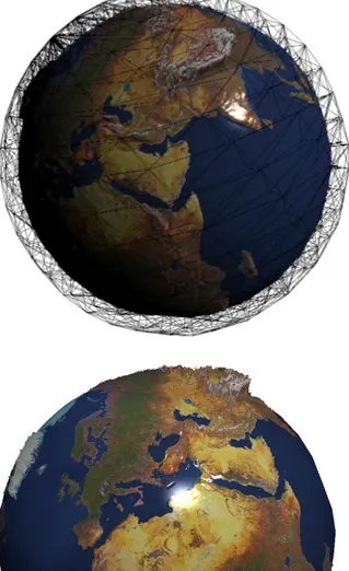
Figure 10: Sphere shaped base mesh with a earth displacement map and texture applied to it. Additionally the wire- frame of the tetrahedral mesh is shown.

Figure 10: Sphere shaped base mesh with a earth displacement map and texture applied to it. Additionally the wire- frame of the tetrahedral mesh is shown.

Figure 11: Different angle, this time showing europe with slightly exaggerated displacements.

G. Zachmann Advanced Computer Graphics SS 15 May 2013 Advanced Shader Techniques 43

Intermezzo: Adjacency Information

§  In addition to the conventional primitives (GL_TRIANGLE et al.), a few new primitives were introduced with geometry shaders

§  The most frequent one: GL_TRIANGLES_WITH_ADJACENCY

Shells & Fins

§  Suppose, we want to generate a

"fluffy", ghostly character like this

§  Idea:

§  Render several shells (offset surfaces) around the original polygonal geometry

-  Can be done easily using the vertex shader

§  Put different textures on each shell the generate a volumetric,

yet "gaseous" shell appearance

G. Zachmann Advanced Computer Graphics SS 15 May 2013 Advanced Shader Techniques 45

§   Problem at the silhouettes:

§   Solution: add "fins" at the silhouette

§  Fin = polygon standing on the edge between 2

silhouette polygons

§   Makes problem much less noticeable

8 shells

+

fins

§  Idea: fins can be generated in the geometry shader

§  How it works:

§  All geometry goes through the geometry shader

§  Geometry shader checks whether or not the polygon has a silhouette edge:

where e = eye vector

§  If one edge = silhouette, then the

geometry shader emits a fin polygon, and the input polygon

§  Else, it just emits the input polygon ⁿ¹

n2

silhouette , en

> 0 ^ en

< 0 or en

< 0 ^ en

> 0

G. Zachmann Advanced Computer Graphics SS 15 May 2013 Advanced Shader Techniques 49

Silhouette Rendering

§  Goal:

§  Technique: 2-pass rendering 1. Pass: render geometry regularly

2. Pass: switch on geometry shader for silhouette rendering

§  Switch to green color for all geometry (no lighting)

§  Render geometry again

§  Input of geometry shader = triangles

§  Output = lines

§  Geometry shader checks, whether triangle contains silhouette edge

§  If yes ⟶ output line

§  If no ⟶ output no geometry

§  Geometry shader input = GL_TRIANGLE_WITH_ADJACENCY

output = GL_LINE_STRIP

G. Zachmann Advanced Computer Graphics SS 15 May 2013 Advanced Shader Techniques 52

More Applications of Geometry Shaders

§  Hedgehog Plots:

Shader Trees

G. Zachmann Advanced Computer Graphics SS 15 May 2013 Advanced Shader Techniques 57

Resources on Shaders

§  Real-Time Rendering; 3

edition

§  Nvidia GPU Programming Guide:

developer.nvidia.com/object/gpu_programming_guide.html

§  On the geometry shader in particular:

www.opengl.org/registry/specs/ARB/geometry_shader4.txt

The Future of GPUs?

G. Zachmann Advanced Computer Graphics SS 15 May 2013 Advanced Shader Techniques 60

G. Zachmann Advanced Computer Graphics SS 15 May 2013 Advanced Shader Techniques 62