Advanced Computer Graphics

Advanced Computer Graphics

Advanced Shader Programming

G. Zachmann

University of Bremen, Germany

Recap

§  Programmable vertex und fragment processors

§  Expose that which was already there anyway

§  Texture memory = now general storage for any data

Vertex Processing

Cull, Clip

& Project Assemble And Rasterize Primitive

Fragment Processing

Per- Fragment Operations

Frame Buffer Operations

Texture Memory

Frame Buffer

Read Back Control

Host Commands Display

glBegin(GL_…)

glEnable, glLight, …

Pixel Pack &

Unpack

glVertex

glTexImage

Status Memory

A More Abstract Overview of the Programmable Pipeline

Vertex Shader

Primitive Assembly

Fragment

Shader Rasterization

OpenGL State

glBegin(GL_…), glColor, … glLight, glRotate, … glVertex()

Vertices in Model Coord.

Vertices in Camera Coord.

Connectivity

Primitives

Fragments

New Fragments

More Versatile Texturing by Shader Programming

§  Declare texture in the shader (vertex or fragment):

§  Load and bind texture in OpenGL program as usual:

§  Establish a connection between the two:

§  Access in fragment shader:

uniform sampler2D myTex;

glBindTexture( GL_TEXTURE_2D, myTexture );

glTexImage2D(...); "

uint mytex = glGetUniformLocation( prog, "myTex" );

glUniform1i( mytex, 0 ); // 0 = texture unit, not ID

vec4 c = texture2D( myTex, gl_TexCoord[0].xy ); "

Example: A Simple "Gloss" Texture

§  Idea: expand the conventional Phong lighting by introducing a specular reflection coefficient that is mapped from a texture on the surface

l

v

n r

I _out = (r _d cos + r _s cos ^p ⇥ ) · I _in

r _s = r _s (u , v )

Procedural Textures Using Shader Programming

§  Goal:

Brick texture

§  Simplification &

parameters:

BrickStepSize.y BrickPercent.y

BrickPercent.x

MortarColor BrickColor

§  General mechanics:

§  Vertex shader: normal lighting calculation

§  Fragment shader:

-  For each fragment, determine if the point lies in the brick or in the mortar on the basis of the x/y coordinates of the corresponding point in the object’s space

-  After that, multiply the corresponding color with intensity from lighting model

§  First three steps towards a complete shader program:

Noise

§  Most procedural textures look too "clean"

§  Idea: add all sorts of noise

§  Dirt, grime, random irregularities, etc., for a more realistic appearance

§  Ideal qualities of a noise function:

§  At least C ² -continuous

§  It’s sufficient if it looks random

§  No obvious patterns or repetitions

§  Repeatable (same output with the same input)

§  Convenient domain, e.g. [-1,1]

§  Can be defined for 1-4 dimensions

§  Isotropic (invariant under rotation)

§  Why we don't just use a noise texture:

Sphere rendered with a 3D texture to provide the noise.

Notice the artifacts from linear interpolation.

Sphere rendered with

procedural noise.

§  Simple idea, demonstrated by a 1-dimensional example:

1.  Choose random y-values from [-1,1] at the integer positions:

2.  Interpolate in between, e.g. cubically (linearly isn’t sufficient):

§  This kind of noise function is called value noise

3.  Generate multiple noise functions with different frequencies:

4.  Add all of these together

§  Persistence = "how much amplitude is scaled for successive octaves scaled for successive octaves"

§  Example:

perlin(x ) =

X 1 i =0

p ⁱ n _i (2 ⁱ x ) , x 2 [0, 1], p 2 [0, 1]

Persistence

Scaling along x for octaves

§  The same thing in 2D:

§  Easily allows itself to be generalized into higher dimensions

§  Also called pink noise, or fractal noise

§  Ken Perlin first dealt with this during his work on TRON

Result

Gradient Noise

§  Specify the gradients (instead of values) at integer points:

§  Interpolation to obtain values:

§  At position x, calculate y ₀ and y ₁ as values of the lines through x=0 and x=1 with

the previously specified (random) gradients

§  Interpolate y ₀ and y ₁ with a sinusoidal blending function, e.g.

or

0 x 1 y

₀

y

₁

h(x ) = 3x ² 2x ³

q (x ) = 6x ⁵ 15x ⁴ + 10x ³

§  Advantage of the quintic blending function:

→ the entire noise function is C ² -continuous

§  Example where one can easily see this:

Ken Perlin

Cubic interpolation Quintic interpolation

q ⁰⁰ (0) = q ⁰⁰ (1)

§  Gradient noise in 2D:

§  Set gradients at integer grid points

-  Gradient = 2D vector, not necessarily with length 1

§  Interpolation (as in 1D):

-  W.l.o.g., P = (x,y) ∈ [0,1]x[0,1]

-  Let the following be the gradients:

g ₀₀ = gradient at (0,0), g ₀₁ = gradient at (0,1), g ₁₀ = gradient at (1,0), g ₁₁ = gradient at (1,1) -  Calculate the values z _ij of the "gradient ramps" g _ij

at point P :

z ₁₀ = g ₁₀ ·

✓ x 1 y

◆

z ₁₁ = g ₁₁ ·

✓ x 1

y 1

◆ x

y

0 1

1

0

z ₀₀ = g ₀₀ ·

✓ x y

◆

z ₀₁ = g ₀₁ ·

✓ x

y 1

◆

-  Blending of 4 z-values through bilinear interpolation:

§  Analogous in 3D:

§  Specify gradients on a 3D grid

§  Evaluate 2 ³ = 8 gradient ramps

§  Interpolate these with tri-linear interpolation and the blending function

§  And in d-dim. space? → complexity is !

z _{x 0} = (1 q(x ))z ₀₀ + q (x )z ₁₀ , z _{x 1} = (1 q (x ))z ₀₁ + q(x )z ₁₁ z _xy = (1 q(y ))z _{x 0} + q(y )z _{x 1}

O(2 ^d )

Simplex Noise

§  d-dimensionaler simplex :=

combination of d + 1 affinely independent points

§  Examples:

§  1D simplex = line, 2D simplex = triangle, 3D simplex = tetrahedron

§  In general:

§  Points P ₀ , …, P _d are given

§  d-dim. simplex = all points X with

with

P ₀

P ₁

P ₂ P ₃

X = P ₀ +

d

i =1

s _i u _i

u _i = P _i P ₀ , s _i ⇤ 0 ,

d

i =0

s _i ⇥ 1

§  In general, the following is true:

§  A d-dimensional simplex has d+1 vertices

§  With equilateral d-dimensional simplices, one can partition a cube that was suitably "compressed" along its diagonals

-  Such a "compressed" d-dimensional cube contains d! many simplices

§  Consequence: with equilateral d-dimensional simplexes, one can

partition d-dimensional space (tessellation)

§  Construction of the noise function over a simplex tessellation (hence "simplex noise"):

1.  Determine the simplex in which a point P lies

2.  Determine all of its corners and the gradients in the corners 3.  Determine (as before) the value of these "gradient ramps" in P 4.  Generate a weighted sum of these values

§  Choose weighting functions so that the “influence” of a simplex grid

point only extends to its incident simplexes

§  A huge advantage: has only complexity O(d)

§  For details see "Simplex noise demystified" (on the course's homepage)

§  Comparison between classical value noise and simplex noise:

classical

simplex

§  Four noise functions are defined in the GLSL standard:

float noise1(gentype), vec2 noise2(gentype), vec3 noise3(gentype), vec4 noise4(gentype).

§  Calling such a noise function:

v = noise2( f*x + t, f*y + t )

§  With f, one can control the spatial frequency,

With t, one can generate an animation (t="time").

§  Analogous for 1D and 3D noise

§  Caution: range is [-1,+1]!

§  Cons:

§  Are not implemented everywhere

§  Are sloooooooow…

Example: Application of Noise to our Procedural Texture

§  Our procedural brick texture (please ignore the uneven outer torus contour, that's an artifact from Powerpoint) :

The code for this example is on the course's

homepage (after unpacking the archive, it is in directory vorlesung_demos

With variation in color With fine-grain variations

Other Examples for the Applications of Noise

Procedural bump mapping, done by computing noise in the pixel shader and using that for perturbing the Ken Perlin's famous solid

texture marble vase, 1985

g = a * perlin(x,y,z)

grain = g - int(g)

Remark on Implementation

§  Goal: repeatable noise function

§  That is, f(x) always returns the same value for the same x

§  Choose fixed gradients at the grid points

§  Observation: a few different ones are sufficient

§  E.g. for 3D, gradients from this set are sufficient:

§  Integer coordinates of the grid points can be simply hashed →

index into a table of pre-defined gradients

Light Refraction

§  With shaders, one can implement

approximations of simple global effects

§  Example: light refraction

§  What does one need to calculate the refracted ray?

§  Snell's Law:

§  Needed: n, d, n ₁ , n ₂

§  Everything is available in the fragment shader

§  So, one can calculate t per pixel

§  So why is rendering transparent objs difficult?

§  In order to calculate the correct intersection point of the refracted ray, one needs the entire

n ₁ sin ₁ = n ₂ sin ₂

n ₂ n ₁

n

d

t

1

2

G. Zachmann Advanced Computer Graphics SS 24 June 2014 Advanced Shader Techniques 29

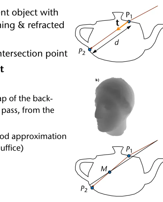
§  Goal: approximate transparent object with two planes, which the incoming & refracted rays intersect

§  Step 1: determine the next intersection point

§  Idea: approximate d

§  To do that, render a depth map of the back- facing polygons in a previous pass, from the viewpoint

§  Use binary search to find a good approximation of the depth (ca. 5 iterations suffice)

P ₁

P ₂

d

P ₁

P ₂

M

t

P ₂ = P ₁ + d t

Index of

refraction: n

_i

P

1

Index of

refraction: n

_t

N ⃗

₂

T ⃗

₂

T ⃗

₄

P

³

V ⃗ θ

_i

θ

_t

P

2

d

_⃗

N

N ⃗

₁

d

_⃗

V

T ⃗

₁

P

4

Figure 2: Vector

V⃗

hits the surface at

P¹

and refracts in di- rection

T⃗¹

based upon the incident angle

θi

with the normal

N⃗¹

. Physically accurate computations lead to further refrac- tions at

P²

,

P³

, and

P⁴

. Our method only refracts twice, approximating the location of

P²

using distances

dN⃗

and

dV⃗

.

follows Snell’s Law, given by:

ni

sin

θi

=

nt

sin

θt,

where

ni

and

nt

are the indices of refraction for the incident and transmission media.

θi

describes the angle between the incident vector

V⃗

and the surface normal

N⃗1

, and

θt

gives the angle between the transmitted vector

T⃗¹

and the negated surface normal.

When ray tracing, refracting through complex objects is trivial, as refracted rays are independently intersected with the geometry, with subsequent recursive applications of Snell’s Law. Unfortunately, in the GPU’s stream processing paradigm performing independent operations for different pixels proves expensive. Consider the example in Figure 2.

Rasterization determines

V⃗

,

P¹

, and

N⃗¹

, and a simple frag- ment shader can compute

T⃗¹

. Unfortunately, exactly locat- ing point

P²

is not possible on the GPU without resorting to accelerated ray-based approaches [Purcell et al. 2003]. Since GPU ray tracing techniques are relatively slow, multiple- bounce refractions for complex polygonal objects are not interactive.

3 Image-Space Refraction

Instead of using the GPU for ray tracing, we propose to approximate the information necessary to refract through two interfaces with values easily computable via rasteriza- tion. Consider the information known after rasterization.

For each pixel, we can easily find:

•

the incident direction

V⃗

,

•

the hitpoint

P¹

, and

•

the surface normal

N⃗¹

at

P¹

.

Using this information, the transmitted direction

T⃗¹

is easily computable via Snell’s Law, e.g., in Lindholm et al. [2001].

Consider the information needed to find the doubly re- fracted ray

T⃗²

. To compute

T⃗²

, only

T⃗¹

, the point

P²

, and the normal

N⃗²

are necessary. Since finding

T⃗¹

is straight- forward, our major contribution is a simple method for ap- proximating

P²

and

N⃗²

. Once again, we use an approximate point ˜

P²

and normal

N⃗²

since accurately determining them requires per-pixel ray tracing.

After finding

T⃗²

, we assume we can index into an infinite environment map to find the refracted color. Future work may show ways to refract nearby geometry.

Figure 3: Distance to back faces (a), to front faces (b), and between front and back faces (c). Normals at back faces (d) and front faces (e). The final result (f ).

3.1 Approximating the Point P

2

While too expensive, ray tracing does provide valuable in- sight into how to approximate the second refraction location.

Consider the parameterization of a ray

Porigin

+

tV⃗direction

. In our case, we can write this as:

P²

=

P¹

+

dT⃗1,

where

d

is the distance

∥P²−P¹∥. KnowingP¹

and

T⃗¹

, approximating location

P˜²

simply requires finding an approximate distance

d, such that:

˜

P˜²

=

P¹

+ ˜

dT⃗¹ ≈P¹

+

dT⃗¹

The easiest approximation ˜

d

is the non-refracted distance

dV⃗

between front and back facing geometry. This can eas- ily be computed by rendering the refractive geometry with the depth test reversed (i.e.,

GL GREATER

instead of

GL LESS

), storing the z-buffer in a texture (Figure 3a), rerendering nor- mally (Figure 3b), and computing the distance using the z values from the two z-buffers (Figure 3c). This simple ap- proximation works best for convex geometry with relatively low surface curvature and a low index of refraction.

Since refracted rays bend inward (for

nt> ni

) toward the inverted normal, as

nt

becomes very large

T⃗¹

approaches

−N⃗1

. This suggests interpolating between distances

d_V⃗

and

dN⃗

(see Figure 2), based on

θi

and

θt

, for a more accurate approximation ˜

d. We take this approach in our results, pre-

compute

dN⃗

for every vertex, and interpolate using:

d

˜ =

θt

θi

d_V⃗

+

„

1

− θt

θi

« d_N⃗.

A precomputed sampling of

d

could give even better ac-

curacy if stored in a compact, easily accessible manner. We

tried storing the model as a 64

²

geometry image [Praun and

Hoppe 2003] and sampling

d

in 64

²

directions for each texel

in the geometry image. This gave a 4096

²

texture containing

sampled

d

values. Unfortunately, interpolating over this rep-

resentation resulted in noticeably discretized

d

values, lead-

ing to worse results than the method described above.

§  On the binary search for finding the depth between P ₁ and P ₂ :

-  Situation: given a ray t, with t _z < 0, and two "bracket" points A ⁽⁰⁾ and B ⁽⁰⁾ , between which the intersection point must be; and a precomputed depth map -  Compute midpoint M ⁽⁰⁾

-  Project midpoint with projection matrix

⟶

-  Use to index the depth map

⟶

-  If -  If

M

^proj

(M

_x^proj

, M

_y^proj

)

˜d

Viewpoint

t

B

⁽⁰⁾

A

⁽⁰⁾

Viewpoint

t

B

⁽⁰⁾

A

⁽⁰⁾

M

⁽⁰⁾

M

_z^proj

˜d

˜d > M _z ^proj ) set A ⁽¹⁾ = M ⁽⁰⁾

˜d < M ^proj ) set B ⁽¹⁾ = M ⁽⁰⁾

Viewpoint

A

⁽⁰⁾

M

⁽⁰⁾

˜d

§  Step 2: determine the normal in P ₂

§  To do that, render a normal map of all back-facing polygons from the viewpoint (yet another pass before the actual

rendering)

§  Project P ₂ with respect to the viewpoint into screen space

§  Index the normal map

§  Step 3:

§  Determine t ₂

§  Index an environment map

t₂ n

Normal map

P ₂

§  Many open challenges:

§  When depth complexity > 2:

-  Which normal/which depth value should be stored in the depth/normal maps?

§  Approximation of distance

§  Aliasing

Examples

With internal reflection

G. Zachmann Advanced Computer Graphics SS 24 June 2014 Advanced Shader Techniques 34

The Geometry Shader

§  Situated between vertex shader and rasterizer

§  Essential difference to other shaders:

§  Per-primitive processing

§  The geometry shader can produce variable-length output!

§  1 primitive in, k prims out

§  Is optional (not necessarily present on all GPUs)

§  Note on the side: features stream out

§  New, fixed-function

§  Divert primitive data to buffers

§  Can be transferred back to the OpenGL prog ("Transform Feedback")

Vertex Shader

Geometry Shader

Pixel Shader

Input Assembler

Setup/

Rasterization

Buffer Op.

Memory Vertex

Buffer

Texture

Depth Texture

Texture

Color Index Buffer

Stream

Out Buffer

Vertex Shader attribute

varying in

Fragment Shader Rasterizer

varying out

(x,y,z)

Geometry Shader Vertex

Shader

uniform attribute

varying

Fragment Shader

Rasterizer Buffer Op.

varying

(x’,y’,z’) (x,y,z)

§  The geometry shader's principle function:

§  In general "amplify geometry"

§  More precisely: can create or destroy primitives on the GPU

§  Entire primitive as input (optionally with adjacency)

§  Outputs zero or more primitives

-  1024 scalars out max

§  Example application:

§  Silhouette extrusion for shadow volumes

§  Another feature of geometry shaders: can render the same geometry to multiple targets

§  E.g., render to cube map in a single pass:

§  Treat cube map as 6-element array

§  Emit primitive multiple times

GS

1 2 3 4 5

Render Target 0

Array

Some More Technical Details

§  Input / output:

Point, Line, Line with Adjacency, Triangle , Triangle with Adjacency

Geometry Shader

Points, Line Strips,

Points, Lines, Line Strip, Line Loop, Lines with Adjacency, Line Strip with Adjacency,

Triangles, Triangle Strip, Triangle Fan, Triangles with Adjacency,

Triangle Strip with Adjacency

Application generates these primitives

Driver feeds these one-at-a-time into the Geometry Shader

Geometry Shader

§  In general, you must specify the type of the primitives that will be input and output to and from the geometry shader

§  These need not necessarily be the same type

§  Input type:

§  value = primitive type that this geometry shader will be receiving

§  Possible values: GL_POINTS, GL_TRIANGLES, … (more later)

§  Output type:

§  value = primitive type that this geometry shader will output

§  Possible values: GL_POINTS, GL_LINE_STRIP, GL_TRIANGLES_STRIP

glProgramParameteri( shader_prog_name,

GL_GEOMETRY_INPUT_TYPE, int value );

glProgramParameteri( shader_prog_name,

GL_GEOMETRY_OUTPUT_TYPE, int value );

then the Geometry Shader will read them as:

gl_PositionIn[ ] gl_TexCoordIn[ ] gl_FrontColorIn[ ] gl_BackColorIn[ ] gl_PointSizeIn[ ] gl_LayerIn[ ]

"varying in"

Data Flow of the Principle Varying Variables

gl_VerticesIn If a Vertex Shader

writes variables as:

gl_Position gl_TexCoord[ ] gl_FrontColor gl_BackColor gl_PointSize gl_Layer

"varying"

and will write them to the Fragment Shader as:

gl_Position gl_TexCoord[ ] gl_FrontColor gl_BackColor gl_PointSize gl_Layer

"varying out"

§  If a geometry shader is part of the shader program, then passing information from the vertex shader to the fragment shader can only happen via the geometry shader:

Vertex Shader

Geom Shader

Fragment Sh.

varying vec4 gl_Position;

varying vec4 VColor;

VColor = gl_Color;

Already declared for you

varying in vec4 gl_Position[3];

varying in vec4 VColor[3];

varying out vec4 gl_Position;

varying out vec4 FColor;

varying vec4 FColor;

gl_Position = gl_Position[0];

FColor = VColor[0]:

Emitvertex();

…

Primitive Assembly

Rasterizer

Fragment shader code

Vertex shader code

§  Since you may not emit an unbounded number of points from a geometry shader, you are required to let OpenGL know the

maximum number of points any instance of the shader will emit

§  Set this parameter after creating the program, but before linking:

§  A few things you might trip over, when you try to write your first geometry shader:

§  It is an error to attach a geometry shader to a program without attaching a vertex shader

§  It is an error to use a geometry shader without specifying GL_GEOMETRY_VERTICES_OUT

glProgramParameteri( shader_prog_name,

GL_GEOMETRY_VERTICES_OUT, int n );

§  The geometry shader generates geometry by repeatedly calling EmitVertex() and EndPrimitive()

§  Note: there is no BeginPrimitive( ) routine. It is implied by

§  the start of the Geometry Shader, or

§  returning from the EndPrimitive() ^call

A Very Simple Geometry Shader Program

#version 120

#extension GL_EXT_geometry_shader4 : enable void main(void)

{

gl_Position = gl_PositionIn[0] + vec4(0.0, 0.04, 0.0, 0.0);

gl_FrontColor = vec4(1.0, 0.0, 0.0, 1.0);

EmitVertex();

gl_Position = gl_PositionIn[0] + vec4(0.04, -0.04, 0.0, 0.0);

gl_FrontColor = vec4(0.0, 1.0, 0.0, 1.0);

EmitVertex();

gl_Position = gl_PositionIn[0] + vec4(-0.04, -0.04, 0.0, 0.0);

gl_FrontColor = vec4(0.0, 0.0, 1.0, 1.0);

EmitVertex();

EndPrimitive();

Examples

§  Shrinking triangles:

G. Zachmann Advanced Computer Graphics SS 24 June 2014 Advanced Shader Techniques 47

Displacement Mapping

§  Geometry shader extrudes prism at each face

§  Fragment shader ray-casts against height field

§  Shade or discard pixel depending on ray test

BTexture := (e1,e₂,1)

In the same manner we define a local baseBWorld with the world coordinates of the vertices:

f₁:=V₂ V₁ f2:=V3 V1

BWorld := (f₁,f₂,N₁)

The basis transformation fromBWorld toBTexture can be used to move the viewing direction at the vertex posi- tionV₁to local texture space.

To avoid sampling outside of the prism, the exit point of the viewing ray has to be determined. In texture space the edges of the prism are not straightforward to detect and a 2D intersection calculation has to be performed.

This can be overcome by defining a second local coor- dinates system which has its axes aligned with the prism edges. For this we assign 3D coordinates to the vertices as shown in Figure 2. The respective name for the new coordinate for a vertexV_iisO_i. Then the the viewing di-

(0,0,1)

(0,1,0) (0,1,1)

(1,0,1)

(1,0,0)

(0,0,0)

Figure 2: The vectors used to define the second local coordinate system for simpler calculation of the ray exit point.

rection can be transformed in exactly the same manner to the local coordinate system defined by the edges between theOi vectors:

g₁:=O₂ O₁ g2:=O3 O1

BLocal := (g1,g₂,1).

Again this is the example for the vertexV₁. In the follow- ing the local viewing direction in texture space is called

pipeline in order to get linearly interpolated local view- ing directions. The interpolatedView_L allows us to very easily calculate the distance to the backside of the prism from the given pixel position as it is either the difference of the vector coordinates to 0 or 1 depending which side of the prism we are rendering. With this Euclidean dis- tance we can define the sampling distance in a sensible way which is important as the number of samples that can be read in one pass is limited, and samples should be evenly distributed over the distance. An example of this algorithm is shown in figure 3. In this case four sam- ples are taken inside the prism. The height of the dis- placement map is also drawn for the vertical slice hit by the viewing ray. The height of the third sample which is equal to the third coordinate of its texture coordinate as explained earlier, is less than the displacement map value and thus a hit with the displaced surface is detected. To improve the accuracy of the intersection calculation, the sampled heights of the two consecutive points with the intersection inbetween them, are substracted from the in- terpolated heights of the viewing ray. Because of the in- tersection the sign of the two differences must differ and the zero-crossing of the linear connection can be calcu- lated. If the displacement map is roughly linear between the two sample points, the new intersection at the zero- crossing is closer to the real intersection of the viewing ray and the displaced surface than the two sampled posi- tions.

Figure 3: Sampling within the extruded prism with a slice of the displacement map shown.

Although the pixel position on the displaced surface is

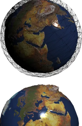
Figure 10: Sphere shaped base mesh with a earth displacement map and texture applied to it. Additionally the wire- frame of the tetrahedral mesh is shown.

Figure 10: Sphere shaped base mesh with a earth displacement map and texture applied to it. Additionally the wire- frame of the tetrahedral mesh is shown.

Figure 11: Different angle, this time showing europe with slightly exaggerated displacements.

Intermezzo: Adjacency Information

§  In addition to the conventional primitives (GL_TRIANGLE et al.), a few new primitives were introduced with geometry shaders

§  The most frequent one: GL_TRIANGLES_WITH_ADJACENCY

Triangles with Adjacency

6N vertices are given

(where N is the number of triangles to draw).

Points 0, 2, and 4 define the triangle.

Points 1,3, and 5 tell where adjacent triangles are.

2 1

0 4

N = 1 5

3

Shells & Fins

§  Suppose, we want to generate a

"fluffy", ghostly character like this

§  Idea:

§  Render several shells (offset surfaces) around the original polygonal geometry

-  Can be done easily using the vertex shader

§  Put different textures on each shell the generate a volumetric,

yet "gaseous" shell

appearance

§  Problem at the silhouettes:

§  Solution: add "fins" at the silhouette

§  Fin = polygon standing on the edge between 2

silhouette polygons

§  Makes problem much less noticeable

8 shells

+

§  Idea: fins can be generated in the geometry shader

§  How it works:

§  All geometry goes through the geometry shader

§  Geometry shader checks whether or not the polygon has a silhouette edge:

where e = eye vector

§  If one edge = silhouette, then the

geometry shader emits a fin polygon, and the input polygon

n2

silhouette , en ₁ > 0 ^ en ₂ < 0 or en ₁ < 0 ^ en ₂ > 0

Demo

Example Application: Lost Planet Extreme Condition

Texture for color Texture for angle of fur hairs

Noise texture for length of fur hairs

§  More tricks are usually needed to make it look really good:

Furthermore,

one should

try to render

self-shadowing

of strands of fur

hairs …

§  Typically, what you as a programmer need to do is to write the

shader and expose the parameters via a GUI to the artists, so that

they can determine the best look

Silhouette Rendering

§  Goal:

§  Technique: 2-pass rendering 1.  Pass: render geometry regularly

2.  Pass: switch on geometry shader for silhouette rendering

§  Switch to green color for all geometry (no lighting)

§  Render geometry again

§  Input of geometry shader = triangles

§  Output = lines

§  Geometry shader checks, whether triangle contains silhouette edge

§  If yes ⟶ output line

§  If no ⟶ output no geometry

§  Geometry shader input = GL_TRIANGLE_WITH_ADJACENCY

More Applications of Geometry Shaders

§  Hedgehog Plots:

Shader Trees

Concluding Demos

demos/shader/GLSLShowpiece/GLSLShowpiece.app

Resources on Shaders

§  Real-Time Rendering; 3 ^rd edition

§  The tutorial on the course home page

§  OpenGL Shading Language Reference:

http://www.opengl.org/documentation/glsl/

§  On the geometry shader in particular:

www.opengl.org/registry/specs/ARB/geometry_shader4.txt

The Future of GPUs?