Credit Risk Evaluation

(1)

Credit Risk Evaluation

Modeling – Analysis – Management

INAUGURAL-DISSERTATION

ZUR ERLANGUNG DER WÜRDE EINES D^OKTORS

DER WIRTSCHAFTSWISSENSCHAFTEN

DER WIRTSCHAFTSWISSENSCHAFTLICHEN FAKULTÄT DER RÛPRECHT-KÂRLS-UNIVERSITÄT HÊIDELBERG

VORGELEGT VON

UWE WEHRSPOHN AUS E^PPINGEN

HEIDELBERG, JULI 2002

(2)

This monography is available in e-book-format at http://www.risk-and-evaluation.com.

This monography was accepted as a doctoral thesis at the faculty of economics at Heidelberg University, Ger- many.

D-75031 Eppingen

www.risk-and-evaluation.com

(3)

Acknowledgements

My thanks are due to Prof. Dr. Hans Gersbach for lively discussions and many ideas that con- tributed essentially to the success of this thesis.

Among the many people who provided valuable feedback I would particularly like to thank Prof. Dr. Eva Terberger, Dr. Jürgen Prahl, Philipp Schenk, Stefan Lange, Bernard de Wit, Jean-Michel Bouhours, Frank Romeike, Jörg Düsterhaus and many colleagues at banks and consulting companies for countless suggestions and remarks. They assisted me in creating the awareness of technical, mathematical and economical problems which helped me to formulate and realize the standards that render credit risk models valuable and efficient in banks and financial institutions.

Further, I gratefully acknowledge the profound support from Gertrud Lieblein and Computer Sciences Corporation – CSC Ploenzke AG that made this research project possible.

My heartfelt thank also goes to my wife Petra for her steady encouragement to pursue this extensive scientific work.

Uwe Wehrspohn

(4)

Introduction

In the 1990ies, credit risk has become the major concern of risk managers in financial institutions and of regulators. This has various reasons:

• Although market risk is much better researched, the larger part of banks’ economic capital is generally used for credit risk. The sophistication of traditional standard methods of measurement, analysis, and management of credit risk might, therefore, not be in line with its significance.

• Triggered by the liberalization and integration of the European market, new chan- nels of distribution through e-banking, financial disintermediation, and the en- trance of insurance companies and investment funds in the market, the competitive pressure upon financial institutions has increased and led to decreasing credit margins¹. At the same time, the number of bankruptcies of companies stagnated or increased² in most European countries, leading to a post-war record of insolvencies in 2001 in Germany³.

• A great number of insolvencies and restructuring activities of banks were influenced by prior bankruptcies of creditors. In the German market, prominent exam- ples are the Bankgesellschaft Berlin (2001), the Gontard-MetallBank (2002), the Schmidtbank (2001), and many mergers among regional banks⁴ to avoid insolvency or a shut down by regulatory authorities.

The thesis contributes to the evaluation and development of credit risk management methods.

First, it offers an in-depth analysis of the well-known credit risk models Credit Metrics (JP Morgan), Credit Risk+ (Credit Suisse First Boston), Credit Portfolio View (McKinsey &

Company) and the Vasicek-Kealhofer-model⁵ (KMV Corporation). Second, we develop the Credit Risk Evaluation model⁶ as an alternative risk model that overcomes a variety of deficiencies of the existing approaches. Third, we provide a series of new results about homogenous portfolios in Credit Metrics, the KMV model and the CRE model that allow to better

1 Bundesbank (2001).

2 Creditreform (2002), p. 4.

3 Creditreform (2002), p. 16.

4 Between 1993 and 2000 1,000 out of 2,800 Volks- und Raiffeisenbanken and 142 out of 717 savings banks ceased to exist in Germany (Bundesbank 2001, p. 59). All of them merged with other banks so that factual insolvency could be avoided in all cases. Note that shortage of regulatory capital in consequence of credit losses was not the reason for all of these mergers. Many of them were motivated to achieve cost reduction and were carried out for other reasons.

5 We refer to the Vasicek-Kealhofer-model also as the KMV model.

6 Credit Risk Evaluation model is a trademark of the Center for Risk & Evaluation GmbH & Co. KG, Heidelberg. We refer to the Credit Risk Evaluation model also as the CRE model.

(5)

understand and compare the models and to see the impact of modeling assumptions on the reported portfolio risk. Fourth, the thesis covers all methodological steps that are necessary to quantify, to analyze and to improve the credit risk and the risk adjusted return of a bank portfolio.

Conceptually, the work follows the risk management process that comprises three major aspects: the modeling process of the credit risk from the individual client to the portfolio (the qualitative aspect), the quantification of portfolio risk and risk contributions to portfolio risk as well as the analysis of portfolio risk structures (the quantitative aspect), and, finally, methods to improve portfolio risk and its risk adjusted profitability (the management aspect).

The modeling process

The modeling process includes the identification, mathematical description and estimation of influence factors on credit risk. On the level of the single client these are the definitions of default⁷ and other credit events⁸, the estimation of default probabilities⁹, the calculation of credit exposures¹⁰ and the estimation of losses given default¹¹. On the portfolio level, dependencies and interactions of clients need to be modeled¹².

The assessment of the risk models is predominantly an analysis of the modeling decisions taken and of the estimation techniques applied. We show that all of the four models have considerable conceptual problems that may lead to an invalid estimation, analysis and pricing of portfolio risk.

In particular, we identify that the techniques applied for the estimation of default probabilities and related inputs cause systematic errors in Credit Risk+¹³ and Credit Portfolio View¹⁴ if certain very strict requirements on the amount of available data are not met even if model assumptions are assumed to hold. If data is sparse, both models are prone to underestimate default probabilities and in turn portfolio risk.

For Credit Metrics and the KMV model, it is shown that both models lead to correct results if they are correctly specified. The concept of dependence that is common to both models – called the normal correlation model – can easily be generalized by choosing a non-normal

7 See section I.A.

8 I.e. of rating transitions, see sections I.B.4, I.B.6.c)(4), I.B.7.

9 See section I.B.

10 Section I.C.

11 Section I.D.

12 See Section II.A.

13 Section I.B.5

14 Section I.B.6

(6)

distribution for joint asset returns. As one of the main results, we prove for homogenous portfolios that the normal correlation model is precisely the risk minimal among of all possible generalizations of this concept of dependence. This implies that even if the basic concept of dependence is correctly specified, Credit Metrics and the Vasicek-Kealhofer model systematically underestimate portfolio risk if there is any deviation from the normal distribution of asset returns.

Credit Risk+ has one special problem regarding the aggregation of portfolio risk¹⁵. It is the only model whose authors intend to avoid computer simulations to calculate portfolio risk and attain an analytical solution for the portfolio loss distribution. For this reason, the authors choose a Poisson approximation of the distribution of the number of defaulting credits in a portfolio segment. As a consequence each segment contains an infinite number of credits.

This hidden assumption may lead to a significant overestimation of risk in small segments, e.g. when the segment of very large exposures in a bank portfolio is considered that is usually quite small. Thus, Credit Risk+ is particularly suited for very large and homogenous portfolios. However, at high percentiles, the reported portfolio losses even always exceed the total portfolio exposure.

With the Credit Risk Evaluation model, we present a risk model that avoids these pitfalls and integrates a comprehensive set of influence factors on an individual client’s risk and on the portfolio risk. In particular, the CRE model captures influences on default probabilities and dependencies such as the level of country risk, business cycle effects, sector correlations and individual dependencies between clients. This leads to an unbiased and more realistic estimation of portfolio risk¹⁶.

The CRE model also differs from the other models with respect to the architecture, which is modular in contrast to the monolithic design in other models. This means that the corner- stones of credit risk modeling such as the description of clients’ default probabilities, exposures, losses given default, and dependencies are designed as building blocks that interact in certain ways, but the methods in each module can be exchanged and adjusted separately. This architecture has the advantage that, by choosing appropriate methods in each component, the overall model may be flexibly adapted to the type and quality of the available data and to the structure of the portfolio to be analyzed.

15 Section II.A.3.a)

16 Sections I.B.7 and II.A.2

(7)

For instance, if the portfolio is large and if sufficiently long histories of default data are available, business cycle effects on default probabilities can be assessed in the CRE model. Other- wise, more simple methods to estimate default can be applied such as long term averages of default frequencies etc. Similarly, country risk typically is one of the major drivers of portfolio risk of internationally operating banks. In turn, these banks should use a risk model that can capture its effect¹⁷. Regional banks, on the other hand, might not have any exposures on an international scale and, therefore, may well ignore country risk.

Moreover, an object-oriented software implementation of the model can directly follow its conceptual layout. Here, building blocks translate into classes and methods into routines within the classes. This makes it easy to adapt the software to the model and to integrate new methods.

It is worth noting that the CRE model contains Credit Metrics and the Vasicek-Kealhofer model as special cases, if methods in the modules are appropriately specified.

The presentation of our analyses and results follows the modular architecture of the CRE model. We go through the building blocks separately and only analyze the respective component of each model and, if necessary, the restrictions that the choice of a particular model in one building block imposes upon other components. This structure renders it possible to assess each method in each module individually and to avoid that errors accumulate or offset each other and make the resulting effect intransparent and difficult to apprehend.

Analysis of portfolio risk structures

After all components of a portfolio model are defined and all relevant input parameters are estimated, the next step in the credit risk management process entails the quantification of portfolio risk and of risk contributions to portfolio risk and the analysis of portfolio risk structures. This step is entirely based upon the portfolio loss distribution and on the concept of marginal risks. As they are based upon standardized model outputs, all methods to analyze risk structures are generally valid and independent of the underlying risk model.

We develop a general simulation based approach how the portfolio loss distribution and the expected loss, the standard deviation, the value at risk, and the shortfall as specific risk measures can be estimated and supply formulas for confidence intervals around the estimated risk measures and confidence bands around the loss distribution. We also show that the calculation

17 Sections I.B.7.a)(1) and II.A.5.

(8)

of value at risk and shortfall may be subject to systematic estimation errors if the number of simulation runs is not sufficiently large with regard to the required confidence level.

The mere calculation of risk measures for the entire portfolio and portfolio segments is usually not sufficient in order to capture the complexity of real world portfolio structures and to localize segments where the risk manager has to take actions. This is due to the fact that different aspects of risk such as segments’ losses given default, their risk contributions, risk adjusted returns etc. may lead to very different pictures of the portfolio structure and may also interact. I.e. a portfolio segment, that appears to be moderately risky if single aspects of risk are considered in isolation, can gain a high priority if various concepts of risk and return are evaluated in combination. For this reason, we give an example of a comprehensive portfolio analysis and the visualization of portfolio risk in a ‘risk management cockpit’.

A complementary approach to improve portfolio quality that does not depend upon the actual portfolio composition is algorithmic portfolio optimization. We develop a method that mini- mizes portfolio shortfall under certain side-constraints such as the size of expected returns or non-negativity of exposures and give an example of an optimization and its effect upon portfolio composition and marginal risk contributions.

Risk management techniques

When portfolio risk is modeled, measured and decomposed, the risk manager may want to take action to adjust the portfolio along value at risk, shortfall and return considerations. On the level of the single client this can be done by adequate, risk adjusted pricing of new credits and the allocation of credit lines. On the portfolio level, the allocation of economic capital as well as the setting of risk, exposure and concentration limits, credit production guidelines, and credit derivatives can be used, for instance, to redirect the portfolio.

The thesis is organized as follows: In the first part, we discuss the credit risk management of a single client. This includes the modeling and estimation of clients’ risk factors and mainly the risk adjusted pricing of financial products. In the second part, the focus is on the risk management of multiple clients. We begin with a detailed description and analysis of various concepts of dependence between clients. Subsequent sections deal with the quantification and analysis of portfolio risk and with risk management techniques.

(9)

Introduction 4

The modeling process 5

Analysis of portfolio risk structures 7

Risk management techniques 8

I. The credit risk of a single client 16

A. Definitions of default 16

B. Estimation of default probabilities 17 1. Market factor based estimation of default probabilities: the Merton model 17

a) Main concept 18

b) Assumptions 18

c) Derivation of default probability 20

d) Discussion 22

2. Extensions of Merton’s model by KMV 25

a) Discussion 26

3. Market factor based estimation of default probabilities: the Jarrow-Turnbull

models 27

b) Discussion 29

4. Rating based estimation of default probabilities: the mean value model 30

b) Derivation of default probability 31

c) Discussion 32

d) How many rating categories should a financial institution distinguish? 39

5. Rating based estimation of default probabilities: Credit Risk + 40

II. The credit risk of multiple clients 101

A. Concepts of dependence 101

1. The normal correlation model 103

a) The Vasicek-Kealhofer model 103

b) Credit Metrics 106

c) Homogenous Portfolios 107

2. The generalized correlation model (CRE model) 112

a) Homogenous Portfolios 119

(1) Portfolio loss distribution 120

(2) Portfolio loss density 126

(3) Comparison of the normal and the generalized correlation model 129

(4) More complex types of homogenous portfolios 133

(5) Speed of convergence 137

b) Estimation of risk index distributions 139

c) Copulas 142

3. Random default probabilities (Credit Risk+ and Credit Portfolio View) 144

a) Credit Risk+ 144

b) Credit Portfolio View 146

4. A brief reference to the literature and comparison of the models applied to

homogenous portfolios 146

5. Event driven dependencies (CRE model) 149

B. Time horizons for risk calculations 152

1. A standardized time horizon 152

2. Heterogeneous time horizons 155

C. Quantification of portfolio risk 155

1. Portfolio loss distribution 155

2. Expected loss 161

(12)

a) Estimation 161

b) Confidence intervals 162

3. Standard deviation 163

4. Value at risk 168

5. Shortfall 171

D. Risk analysis and risk management 173

1. Marginal risks 174

a) Marginal risks conditional to default 174 b) Marginal risks prior to default 175 c) Combinations of exposure and marginal risk 178 d) Expected risk adjusted returns 179

e) Summary 182

2. Credit derivatives 183

3. Portfolio optimization 183

a) Optimization approach 184

b) A portfolio optimization 185

Conclusion 188

Literature 189

(13)

List of figures

Figure 1: Default probability vs. distance to default in Merton’s model ...24

Figure 2: Deviation of portfolio value at risk dependent on number of rating categories ...34

Figure 3: Distributions of estimated default probabilities in mean value model...36

Figure 4: Variance of mean value estimator of default probability...38

Figure 5: Frequency of invalid volatility estimations in Credit Risk + ...43

Figure 6: Bias of estimated default rate volatility in Credit Risk + dependent on number of periods and number of clients...44

Figure 7: Bias of estimated default rate volatility in Credit Risk + dependent on number of periods ...45

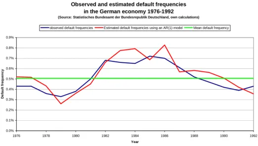
Figure 8: Observed and estimated default frequencies in the German economy 1976-1992...46

Figure 9: Persistence of macroeconomic shocks in Credit Portfolio View...50

Figure 10: Logit and inverse logit transformation...51

Figure 11: Convex transforms and probability distributions...51

Figure 12: Bias of long-term mean default probability in Credit Portfolio View ...54

Figure 13: Relative error of estimated long-term mean default probability in Credit Portfolio View...54

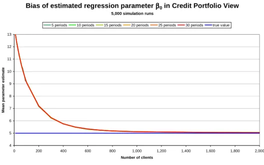
Figure 14: Bias of estimated regression parameter β0 in Credit Portfolio View ...55

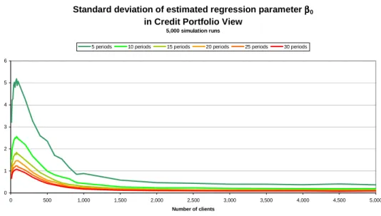
Figure 15: Standard deviation of estimated regression parameter β₀ in Credit Portfolio View ...56

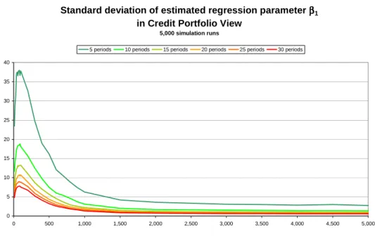
Figure 16: Bias of estimated regression parameter β1 in Credit Portfolio View ...56

Figure 17: Standard deviation of estimated regression parameter β1 in Credit Portfolio View ...57

Figure 18: Distributions of estimated parameter values for (β0,β1) in Credit Portfolio View..58

Figure 19: Distributions of long-term mean probabilities of default of estimated processes in Credit Portfolio View ...59

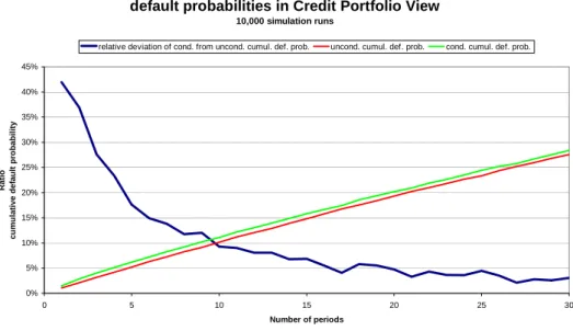
Figure 20: Conditional and unconditional cumulative default probabilities in Credit Portfolio View...63

Figure 21: Expected values of estimated parameter β0 in the CRE model under correlated defaults...71

Figure 22: Standard deviation of estimated parameter β0 in the CRE model under correlated defaults...72

Figure 23: Expected value of macro parameter β1 in the CRE model under correlated defaults ...72

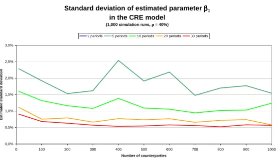
Figure 24: Standard deviation of estimated parameter β1 in the CRE model under correlated defaults...73

Figure 25: Standard deviation of estimated parameters (β0,β1) in the CRE model dependent on the size of correlations ...73

Figure 26: Distributions of estimated parameter values (β0,β1) in the CRE model under various correlations...74

Figure 27: Add-on factor of a portfolio of options on 100 different shares ...84

Figure 28: Potential exposure of a portfolio of options on 100 different shares ...85

Figure 29: Beta distributions of recovery rates of public bonds in different seniority classes.89 Figure 30: Portfolio analysis, CAD, and equity allocation...99

Figure 31: Risk premiums, correlations, portfolio analysis, and regulatory capital requirements ...100

Figure 32: Default rates of corporates in Germany for different rating grades ...102

Figure 33: Abstract default threshold for a firm with annual probability of default of 1% ...104

Figure 34: Simulated bivariate normal distributions and marginals...105

(14)

Figure 35: Loss distributions of homogenous portfolios in the normal correlation model 1 .110 Figure 36: Loss distributions of homogenous portfolios in the normal correlation model 2 .112

Figure 37: An empirical long tail distribution in finance: DAX-returns ...113

Figure 38: Spherical and elliptical distributions...114

Figure 39: Densities of normal variance mixture distributions ...117

Figure 40: Tail behavior of normal mixture distributions ...118

Figure 41: Portfolio loss distributions in the generalized correlation model based on finite mixture distributions...122

Figure 42: Portfolio loss distributions in the generalized correlation model based on normal inverse Gaussian distributions ...123

Figure 43: Loss distributions resulting from uncorrelated Student-t-distributed risk indices 124 Figure 44: Loss distributions resulting from uncorrelated finite mixture distributed risk indices ...125

Figure 45: Portfolio loss densities in the bimixture correlation model ...127

Figure 46: Portfolio loss densities in the normal correlation model...128

Figure 47: Trimodal portfolio loss densities in the trimixture correlation model ...128

Figure 48: The low correlation effect in the finite mixture model ...129

Figure 49: Portfolio loss distributions in the normal versus the generalized correlation model ...130

Figure 50: Portfolio densities in the normal and the generalized correlation model...131

Figure 51: Loss distribution of an almost homogenous portfolio in the NIG correlation model ...137

Figure 52: The speed of convergence towards the asymptotic portfolio loss distribution in the generalized correlation model ...139

Figure 53: Bivariate distributions with standard normal marginals and different copulas ....143

Figure 54: Loss distribution of a junk bond portfolio according to Credit Risk+ ...145

Figure 55: Loss distributions resulting from Credit Risk+, Credit Portfolio View and the normal correlation model...148

Figure 56: Relative deviation of the portfolio loss distributions ...148

Figure 57: The event risk effect in portfolio risk calculations: country risk ...150

Figure 58: Cascading effect of microeconomic dependencies ...151

Figure 59: Influence of the time horizon on the 99.9%-value at risk ...153

Figure 60: Term structure of default rates: direct estimates versus extrapolated values...154

Figure 61: Uniform 95%-confidence bands for the portfolio loss distribution dependent on the number of simulation runs ...156

Figure 62: Pointwise 95%-confidence intervals for the portfolio loss distribution dependent on the number of simulation runs ...157

Figure 63: Accuracy of the estimation of the expected portfolio loss dependent on the number of simulation runs ...163

Figure 64: The ratio of value at risk and standard deviation of credit portfolios ...165

Figure 65: Accuracy of the estimation of the standard deviation of portfolio losses dependent on the number of simulation runs ...167

Figure 66: Accuracy of the estimation of the value at risk of portfolio losses dependent on the number of simulation runs ...170

Figure 67: Accuracy of the estimation of the shortfall of portfolio losses dependent on the number of simulation runs ...172

Figure 68: Loss distribution of the example portfolio ...174

Figure 69: Exposure distribution and exposure limits...175

Figure 70: Risk and exposure concentrations...176

Figure 71: Risk concentrations and concentration limits ...177

Figure 72: Absolute risk contributions and risk limits ...177

(15)

Figure 73: Risk versus exposure and risk concentration ...178

Figure 74: Expected risk adjusted return on economic capital...180

Figure 75: Accepted risk versus expected risk adjusted return per exposure unit and contribution to total risk ...182

Figure 76: Marginal VaR before and after optimization ...187

Figure 77: VaR and shortfall efficient frontiers ...187

List of tables

Table 1: Characteristics of simulated distributions of probability estimator in the mean value model ...37

Table 2: Characteristics of distribution of long-term mean default rate in Credit Portfolio View...59

Table 3: 10-year cumulative default probabilities extrapolated using Markov assumptions ...61

Table 4: Directly estimated 10-year cumulative default probabilities ...62

Table 5: Characteristics of distributions of parameter estimators (β0,β1) in the CRE model under various correlations ...74

Table 6: Typical applications of exposure concepts...87

Table 7: Mean default recovery rates on public bonds by seniority...88

Table 8: Fair prices of defaultable fixed rate bonds ...96

Table 9: Fair spreads of defaultable fixed rate bonds...96

Table 10: Commercial margins of defaultable fixed rate bonds ...96

Table 11: Definition of the example: default probabilities and exposures...173

Table 12: Definition of the example: relevant interest rates ...180

(16)

I. The credit risk of a single client

The credit risk of a single client is the basis of all subsequent risk analysis and of portfolio risk modeling. In this part, we provide a comprehensive account of single credit risk modeling.

To clarify the events considered as ‘credit risk’, we start with different definitions of default.

We continue with an in-depth analysis of various methods to assess default probabilities. In particular, we show the properties and sometimes deficiencies of the estimation techniques and propose new modeling ideas and estimation methods. The next two sections discuss exposure concepts and models for the loss given default rates or recovery rates, respectively.

Finally, as one of the most important risk management techniques at the level of a single client, we give and prove formulas for the risk adjusted pricing of bonds and European options.

A. Definitions of default

While legal definitions of default vary significantly, two main concepts of default can be distinguished.

The first concept is client orientated, i.e. the status of default is a state of a counterparty such as insolvency or bankruptcy. The major consequence of this definition is that all business done with the respective counterparty is affected simultaneously in the event of default. Thus, all transactions are fully dependent upon each other. It is impossible by definition that, say, two thirds of a counterparty’s transactions default while the remaining third survives. The single contracts differ only in the loss conditional to default, but not in the fact of default.

This strong interdependence of the trades implies, firstly, that it is sufficient to trace the client’s credit quality and financial prospects to assess the probability of default of each individual contract and, secondly, it allows the aggregation of credit exposures¹⁸ from the single trades to a total exposure of the client as the relevant input to further risk management techniques.

The aggregation of exposures belonging to the same counterparty is not only useful in exposure limitation, but it is an important simplification in all simulation based portfolio models because it reduces the number of exposures to be modeled to the number of clients. Taking into consideration that the consumption of computer resources and calculation time increases

18 See section I.C below.

(17)

quadratically in the number of exposures in most models, it becomes evident that it is an advantage to be able to keep the number of exposures small.

This client-orientated definition of default is adequate for derivatives and trading portfolios and most classical credits.

The second concept of default is transaction orientated. It is, thus, the direct opposite to the first approach. Here, default occurs if a contract is given notice to terminate¹⁹. This definition of default is particularly suitable if financed objects belong to the same investors, but are ju- ridically independent. In this context it would not necessarily be justified to assume that all contracts default simultaneously²⁰. Another application is joint ventures by a number of counterparties. In this situation it is hardly possible to assign the contract to a single client or to give a precise reason for default as all participants are liable.

All estimation techniques of default probabilities subsequently described can be used with the first definition of default that puts the focus on the client. The market data based approaches, however, are specialized on the calculation of individual default probabilities. Hence, they cannot be applied if the transaction-orientated concept of default is required.

All rating based techniques to estimate default probabilities can be used with both concepts. It is worth noting, though, that the Credit Risk Evaluation model, in particular, is designed to handle both concepts simultaneously. It can apply different methods to calculate default probabilities in parallel and can picture specific dependencies between clients and objects²¹.

B. Estimation of default probabilities

1. Market factor based estimation of default probabilities: the Merton model

To determine whether a company has the ability to generate sufficient cash flow to service its debt obligations the focus of traditional credit analysis has been on the company’s fundamental accounting information. Evaluation of the industrial environment, investment plans, bal- ance sheet data and management skills serve as primary input for the assessment of the com-

19 Sometimes default on a transaction level is defined as the event that a due payment is delayed. This definition has a problematic implication. Here default is no absorbing state any more as an insolvency or a notice to terminate. The delayed payment can be made later and the contract survives. Thus, there will be a cluster of observed recoveries after default at 100% since no loss actually occurs if the contract is carried on, whereas in other circumstances, where the delay is due to a more severe credit event, consequences are much more serious.

20 It is, for instance, often observed that residential mortgage loans default up to 10-20 times less frequently than non- residential mortgage loans.

21 See section I.B.7 below.

(18)

panies likelihood of survival over a certain time horizon or over the life of the outstanding liabilities.

It is a well-known critique of this approach that financial statement analysis may present a flawed picture of a firm’s true financial condition and future prospects. Accounting principles are predominantly backward oriented and conservative in design. Moreover, accounting information does, therefore, not include a precise concept of future uncertainty. “Creative accounting” might even intend to disguise the firm’s factual situation within certain legal limits.

Finally, a market valuation a firm’s assets is difficult in the absence of actual market related information.

In his seminal article on credit risk management²² Robert Merton proposes a method to price a public company’s debt based on the equilibrium theory of option pricing by Black and Scholes²³ ²⁴. Supposing that his arguments hold, some of the results can serve as an important input for the calculation of default probabilities.²⁵

a) Main concept

Under the simplifying assumption²⁶ that all of the company’s liabilities are zero-bonds with the same maturity, Merton defines the default of the company as being equivalent to the event that the total value of the firm’s assets is inferior to its obligations at the moment of their maturity. In this case the owners would hand the firm over to the creditors rather than paying back the debt. The probability of default is, thus, equal to the probability of observing this event.

b) Assumptions

In order to be able to close the model²⁷ and to derive formulas, Merton makes a number of technical and fundamental assumptions. The technical assumptions serve above all to facili-

22 Robert Merton (1974)

23 Fisher Black and Myron Scholes (1973)

24 This is why Merton’s model is often referred to as the option pricing approach.

25 The calculation of default probabilities was not proposed by Merton himself in the article quoted above. It is rather an extension of Merton’s original approach, which has been initiated by KMV Corporation, San Francisco (from now on referred to as “KMV”). For further modifications of Merton’s model by KMV see next chapter.

26 See below.

27 It is a central challenge for the model to deduce the hidden variables. Merton’s interest was to price risky debt. All that can be concluded from his analyses are the input variables relevant for this purpose. The assumptions made – both technical and fundamental - have to be seen on that background.

For the calculation of default probabilities one further input is needed (the expected return on firm value) whose derivation remains a major concern for the practicability of the model.

(19)

tate the mathematical presentation and to obtain a tractable formalism and can be considerably weakened²⁸. They are:

1. The market is “perfect” (i.e. there are no transaction costs nor taxes; all assets can be infi- nitely divided; any investor believes that he can buy and sell an arbitrary amount of assets at the market price; borrowing and lending can be done at the same rate of interest; short- sales of all assets are allowed).

2. The risk free rate is constant²⁹.

3. The company has only two classes of claims: (1) a single and homogeneous class of debt, precisely of zero-bonds all with the same seniority³⁰ and maturity. (2) The residual claim, equity.

4. The firm is not allowed to issue any new (senior)³¹ debt nor pay cash dividends nor repur- chase shares prior to the maturity of the debt.³²

5. The Modigliani-Miller theorem obtains, i.e. the value of the firm is invariant to its capital structure.³³

The fundamental assumptions are:

6. The value of the firm, V, follows an autoregressive process, i.e. all information needed to predict the future dynamics of the firm value is contained in its past development. The value of the firm is, particularly, not subject to any exogenous shocks. The assumption that V specifically follows a geometric Brownian motion

Vdz Vdt

dV =µ +σ

is again simplifying³⁴. It implies that the volatility of the returns on firm value is constant over time and that the distribution of its growth rates is normal.

28 Robert Merton (1974), p.450

29 If interest rates are constant there are no term structure effects so that term structure and risk structure effects on the price of debt and the probability of default can trivially be separated.

30 For the calculation of default probabilities, it is not necessary that all bonds have the same seniority since equity is always the most junior claim. It is just relevant for the pricing because a credit’s expected loss usually depends on its seniority.

31 See footnote 30.

32 It would be sufficient that the nominal amounts of debt and of dividend payments were deterministic functions of time.

33 Merton himself shows that the argument holds even without the Modigliani-Miller theorem. However, this case is for- mally more complex because it leads to non-linear stochastic differential equations. See Merton (1974), p. 460.

34 Here µ is the instantaneous rate of return on the firm per unit time, σ is the instantaneous standard deviation of the return on the firm per unit time; dz is a standard Brownian motion.

(20)

7. The value of the firm’s equity, E, (and, hence, debt) is a deterministic function of the value of the firm and time:

E = F(V,t)

Thus, by Itô’s Lemma, the stochastic differential equation defining the distribution of E is explicitly given as

E E

EEdt Edz

dE =µ +σ

where σΕ, µΕand dzE are known functions of V, t, σ, µ and dz. It is essentially implied that the dynamics of the equity markets are fully induced by the stochastic behavior of asset values and that there is no further source of uncertainty in the equity markets as for instance by speculation or imperfect aggregation of information.

8. As a necessary condition for the previous supposition to hold³⁵ and as to be able to use the risk-neutral valuation argument by Black and Scholes to eliminate µ from the stochastic differential equation defining the behavior of E, Merton assumes that an ideal fully self- financed portfolio consisting of the firm, equity, and risk-less debt can be constructed and be valued using a no arbitrage argument.

9. Trading in assets takes place continuously in time so that the mentioned portfolio can be hedged at each point in time.

10. Total equity value is exactly the sum of all incremental equity values.

c) Derivation of default probability

From the definition of default as the event that the firm value is inferior to the total amount of debt at maturity of the debt and from the assumption that firm value follows a geometric Brownian motion, it would be straight forward to calculate the company’s default probability if the so far hidden variables µ, σ, and V0 were known.

It follows from the distribution of the stochastic process of V that the logarithm of firm value at time T is normally distributed with mean³⁶

E(ln VT) = ln V0 + (µ − 0.5 σ²) T and variance

Var (ln VT) = σ² T.

35 If arbitrage were possible in the market, the price of equity would also depend on the size of the arbitrage opportunity.

In this case, Itô’s Lemma would be invalid. For Itô’s Lemma see Øksendal (1998), Theorem 4.1.2.

36 We assume that the present moment is equal to t = 0.

(21)

Therefore, we have³⁷

{ } { } { }

( )

( ) ( ( ) )

( )

(

⁰ ²

) ( )

²^*

2 0

5 . 0 ln

ln

5 . 0 ln

ln 5

. 0 ln

ln

ln ln default

d T

T V

D

T

T V

D T

T V

V

D V D

V

T

T T

− Φ

=

 

 − + −

Φ

=







 − + − < − + −

=

<

=

<

=

σ

σ µ

σ

σ µ σ

σ P µ

P P

P

The remaining task is to assign values to µ, σ, and V0. From Merton’s analysis σ and V0 can be concluded:

From the above assumptions³⁸ it can be shown that µ drops out of the stochastic differential equation defining equity value, E. Hence, µ cannot influence equity value, i.e. E is independent of investors’ risk preferences. Thus, any risk preferences that seem suitable can be assumed without changing the result. It is particularly simplifying to consider investors as risk- neutral implying that µ is equal to the risk-free rate r and that the discount factor for the risky investment is equal to e^-rT.

Furthermore, observing that at maturity, T, of the debt equity value is equal to E_T = max(0, V_T-D),³⁹

the stochastic differential equation defining the distribution of E can be solved using analo- gous arguments to Black and Scholes (1973) ⁴⁰

E0 = V0Φ(d1) – e^-rT D Φ(d2).

As already alluded, it is implied by Itô’s Lemma⁴¹ that

37 With

( )

( ) ( ( ) ) ( )

T D T V

T

D T V

T T V

d D

σ σ µ σ

σ µ σ

σ

µ ln /2

ln 5 . 0 ln 5

. 0 ln

ln

2 0

* 2

−

+



 





− =

−

= +

− +

− −

=

*

d2states how many standard deviations the expected value of ln(VT) is away from the default point ln(D) and is, therefore, often named ‘distance to default’.

38 Especially assumption 8.

39 Since if VT ≥D (with D = total debt), equity holders pay back the debt, and if VT ≤D, equity holders hand over the com- pany. Equity has, thus, the same cash flow profile as a European call option with maturity T and strike price D.

40 With

( )

T d d

T T D r

V d

σ σ

σ

−

=

+

+



 





=

1 2

2 0

1

2 / ln

41 The stochastic differential equation defining the distribution of equity value E = F(V,t) is given by V Vdz

dt F V V

F t

rV F V

dF F σ σ

∂ +∂





∂ + ∂

∂ +∂

∂

= ∂ ² ₂ ² ²

2 1

(22)

( )^σ

σ0^EE0=V0Φ d1 .

Both equations can simultaneously be solved numerically for V0 and σ.

It should be pointed out, however, that even if all stated assumptions are fulfilled, the stochastic process defining the equity value E is apparently⁴² heteroskedastic, i.e. equity volatility σE

is not constant but changes over time. It can, therefore, not be taken for granted that σE is known or that it can be estimated by the 30-day-volatility, which is normally used in the Black-Scholes model⁴³. Therefore, σ and V appear to remain to a certain degree hidden fundamental variables that prevent the model from being fully closed.

This is far more true for the expected return on firm value, µ. Other than in the capital asset pricing model (CAPM), it cannot directly be calculated from market returns, but has to be estimated indirectly from the previously estimated firm value process. It does seem unlikely that this procedure still leads to very precise results.

d) Discussion

If correctly specified, the Merton model is able to compensate for a number of deficiencies of traditional credit analysis.

It provides a methodology to effectively include the market’s perception of a company into credit analysis. The information contained in equity markets is inherently future oriented and, therefore, particularly valuable. Leading to a formula for a company’s default probability, the model has a clear-cut concept of uncertainty that can serve as input to further credit analysis.

Furthermore, default probabilities can be individually assessed on a day-to-day basis for each public company. I.e. companies’ risk profiles can, firstly, be evaluated without a long time lag⁴⁴ so that possible deteriorations in credit qualities can be quickly anticipated and, secondly, risk profiles can be compared on a cardinal scale rather than just on an ordinal scale.

The equity volatility follows from the second term where V F

∂

∂ is the option delta Φ(d1). Cf. for Itô’s Lemma to Øksendal (1998), Theorem 4.1.2.

42 See above.

43 In the Black-Scholes model the equity value is assumed to be homoskedastic, i.e. have constant volatility. An applet that illustrates the relationship between firm value, debt and default probabilities in the Merton model and also the het- eroskedasticity of the equity price process which induces the mentioned estimation problems is available at http://www.risk-and-evaluation.com/Animation/Merton_Modell.html.

44 This is not necessarily true because the amount of debt drawn by a company is not published on a day-to-day basis but rather parallel to the accounting periods. There might also be unknown undrawn lines of credit that could in reality be used to honor payments and avert a default.

(23)

There is no estimation error due to averaging between firms as in the rating based approaches (see below). Since the estimation is merely an evaluation of a stochastic process whose general distribution is known by assumption, there is no sampling error involved in the estimation. Having completely tied down default analysis to the purely quantitative analysis of the firm value process, all errors attributable to judgmental analyses by credit experts are avoided.

Besides the fact that input variables might not be fully known, the main points of criticism concern the validity of the fundamental assumptions made in the model.

The concept of default that a company goes bankrupt if and only if the total amount of assets is inferior to the total amount of debt at a certain point in time does explicitly exclude other reasons of insolvency frequently observed such as temporary liquidity problems, law suits, criminal acts etc. This narrow definition might lead to a misestimation of the probability of default.

It is particularly problematical that in order to be able to apply Itô’s Lemma Merton assumes equity value to be a deterministic function of only asset value and time⁴⁵. Although surely strongly influenced by a company’s fundamental economic facts, it is largely uncontested that equity values are superimposed by speculative tendencies⁴⁶ and market imperfections that lead to inefficient aggregation of information.⁴⁷ Sobehart and Keenan (1999) show that default probabilities are overestimated if the fraction of equity volatility induced by asset volatility is overstated⁴⁸.

The requirement is also violated if a company’s traded equity is not highly liquid so that the noted price might not be identical to the asset’s actual market price. This quite restricts the number of companies accessible to analysis even among the public companies.

The supposition that the firm value follows an autoregressive process restricts the assessment of a company’s creditworthiness solely upon the performance of its stock price. Exogenous influences such as country risk, fluctuations in the economic environment, business cycle effects, and productivity shocks that might change the characteristics of the firm value process are systematically ignored. It becomes clear from this fact that Merton’s model is not an extension or a generalization of traditional credit analysis but rather disconnected from it. This

45 It is worth noting that Merton apparently assumes this deterministic relationship for ‘fundamental’ technical reasons rather than for its economic realism. For the suppositions necessary for the validity of Itô’s Lemma confer to Øksendal (1998), Theorem 4.1.2.

46 Equity prices may even contain a bubble component. This is obvious given the recent experience with internet stocks.

See Money Magazine April 1999, p. 169 for Yahoo’s P/E ratio of 1176.6.

47 For a detailed discussion of possible influences on equity values confer to Lipponer (2000), p. 66-69.

48 Sobehart and Keenan (1999), p. 22ff. The authors state this fact as a major reason why equity and bond markets lead to very inconsistent results when it comes to credit analysis.

(24)

observation is so much more important as imprecisions in distributional assumptions or data quality are necessarily carried through to the estimation of default probabilities if there is no plausibility check against other economic variables that contain similar information.⁴⁹

Defaut probability vs. distance to default (log scale)

1.E-07 1.E-06 1.E-05 1.E-04 1.E-03 1.E-02 1.E-01 1.E+00

0 0.5 1 1.5 2 2.5 3 3.5 4 4.5 5

Distance to default

Estimated default probability (log scale)

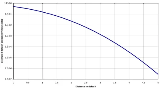
Figure 1: Default probability vs. distance to default in Merton’s model

Figure 1 shows the “distance to default”⁵⁰, plotted against the corresponding probability of default⁵¹. It can be seen that the relationship between both variables is almost exponential implying that small misconceptions of the distance to default can lead to considerable mises- timations of default probability. A holistic credit analysis would, thus, try to combine market and accounting related information, if available, to increase precision to a maximum.

Merton’s approach to deduce firm value, V, and firm value volatility, σ, would not be justified if the differential equation defining the equity value involved the expected return on the firm value, µ, since µ cannot be directly estimated and is not independent of investors’ (unobserv- able) risk preferences. The higher the level of risk aversion by investors, the higher µ will be for any given firm. Merton, therefore, assumes the existence of arbitrageurs who imply that the self-financed portfolio consisting of the firm, equity, and risk-less debt earns the same risk-free rate as other risk-free securities, independent of µ. If the portfolio earned more than this return, arbitrageurs could make a risk-less profit by shorting the risk-free securities and

49 This raises the question where lenders should take position in the trade-off between the error owing to the purely quantitative Merton approach and the error as a result of biased judgmental analyses of a company’s ‘soft facts’.

50 See footnote 37.

51 See the formula above.

(25)

using the proceeds to buy the portfolio; if it earned less, they could make a risk-less profit by doing the opposite, i.e. by shorting the portfolio and buying risk-free securities.⁵²

It is, however, doubtful to take the existence of arbitrageurs for granted in a credit risk context. If equity is a long call option on firm value, the firm’s creditors can be considered to hold the short position of the same option. The situation of creditors and equity owners in this case is slightly different from the short and long position of an ordinary call option, though, because equity holders remain the owners and the managers of the firm in addition to their long option position. This gives them the opportunity to dispose relatively freely of the firm’s assets as it serves their interests. Creditors, on the other hand, as holders of the short position can do little to prevent this until after a default has occurred.⁵³ Creditors are, thus, in a much weaker position than holders of short positions in an ordinary context and, having to face this moral hazard problem of their counterparties, are not necessarily ready to function as arbitrageurs.

Finally, the equity price stated in financial markets is the price for one share only. It is evident from many take-over attempts that a company’s total equity value can be very different from the sum of all incremental equity values.⁵⁴ Hence, total equity value can be considered as another hidden fundamental variable in the model.

2. Extensions of Merton’s model by KMV

The many technical deficiencies of the Merton model greatly diminished its practicability for banks and lenders who wished to assess the default probability of their counterparties. This led KMV Corporation in the early 1980’s to extend the Merton model to a variant, the Va- sicek-Kealhofer model.⁵⁵

The Vasicek-Kealhofer model⁵⁶ has the same conceptual architecture as the Merton approach, but above all tries to weaken and to adapt the technical assumptions⁵⁷.

52 By this argument, Merton tries again to draw an analogy to the Black-Scholes analysis.

53 Confer to Sobehart and Keenan (1999), p. 19f. See also footnote 48.

54 For instance the stock value of Mannesmann increased by 100 billion DEM or more than 100% between October 1999 and February 2000 during an unfriendly takeover by Vodafone.

55 Confer to Vasicek (1984).

56 For clarity, we will refer to this model either as the Vasicek-Kealhofer model or the KMV model.

57 Confer to Vasicek (1984), Crosby (1997), Crouhy et al. (2000), and Sellers et al. (2000).

(26)

While Merton assumes the firm’s liabilities to only consist of two classes, a debt issue matur- ing on a specific date and equity, KMV allows liabilities to include current liabilities, short- term debt, long-term debt, convertible debt, preferred stock, convertible preferred stock, and common equity.⁵⁸

KMV takes account of dividend payments and cash payments of interest prior to the maturity of the debt⁵⁹.

KMV generalizes the concept of default. In the Merton model, default was equivalent to the firm value being lower than the debt at the moment when the debt had to be repaid. In the Vasicek-Kealhofer model default can happen even before the maturity of a particular debt issue.⁶⁰ Equity, in this context, has no expiration date, but is modeled as a perpetual option.⁶¹ In the KMV model, the firm value process is only modeled as a geometric Brownian motion for the purpose of calculation of the unknown input variables and the distance to default⁶².⁶³ It had turned out that the mapping of the distance to default measure to default probabilities via the lognormal law implied by the geometric Brownian motion led to implausible results.⁶⁴ Today an empirical distribution is used to assign default probabilities to the stated distances to default.

a) Discussion

The KMV model is valuable because it rendered the Merton model operational and turned it into a useful tool for practitioners. Although specialized on public companies⁶⁵, this is a group of counterparties that contributes particularly high credit risk to most banks’ total portfolio due to small headcount and large volumes.⁶⁶

Very importantly, the KMV model enables risk managers to monitor public companies on a day-to-day basis and use the estimated default probability⁶⁷ as early warning information that

58 See for instance Vasicek (1984), p. 5 and 11.

59 Vasicek (1984), p. 6 and 11.

60 Vasicek (1984), p. 5f.

61 Sellers et al. (2000), p. 3.

62 See footnote 37.

63 See Crouhy et al. (2000)

64 See Sellers et al. (2000), p.3, where it is stated that the normal law assigned a AAA rating to half of the North Ameri- can companies in the KMV database.

65 Around 9500 companies in the U.S., see Sellers et al. (2000), p. 3.

66 This is particularly true for large, internationally operating banks.

67 KMV calls the output of its model an “expected default frequency” or “EDF”.