Optical Pumping

(1)

Optical Pumping

(2)

Optical Pumping

Institut f¨ ur Mathematik und Physik Albert-Ludwigs-Universit¨ at

Freiburg im Breisgau

Feb. 2016

(3)

1 Introduction

In 1949, Kastler introduced concepts of optical pumping based on the groundbreaking work of Hanle.

First experiments on ground-state polarisation by optical pumping were performed by von Brossel, Kastler, and Winter and by Hawkins, and Dicke. In 1966, Kastler got awarded with the Nobelprize for his contributions to this work. For an extensive introduction we refer you to Sec. I of Ref. [Ha72] and common text books, e.g., Ref. [Co77].

In this advanced laboratory physics experiment, you study the process of optical pumping, i.e., the fundamental interaction between light and matter. You use circularly polarised light from a laser source to prepare a well defined ground-state level of a Rubidium sample. Further, you apply static and oscillating magnetic fields to manipulate the population distribution of these levels. Applying these common atomic physics techniques you determine, e.g., the nuclear magnetic moment of Rb. You apply the two distinct methods of Dehmelt [De57] and Franzen [Fr59] to determine the relaxation times within your setup. Details on all measurements and the experimental setup are described in Ref. [Ba97].

Please be prepared for the measurements and present a solid knowledge about the following topics: diode laser (working principle), atomic physics (fine and hyperfine structure, and Zeeman effect, relaxation processes), and light-matter interaction (light polarisation states, absorption and emission processes, selection rules, linewidth, line broadening effects, and optical pumping principle).

2 Experimental Setup

We present an overview of the experimental setup arranged around a spherical glass cell filled with natural abundant Rubidium, with the two isotopes⁸⁵Rb ('72.8 %) and⁸⁷Rb ('27.2 %). The cell has an diameter of about 5 cm and is, additionally, filled with a Krypton buffer gas at a pressure of about 150 Pa. The buffer gas is used to reduce the mean free path length of Rb atoms in the cell and in this way it reduces Doppler broadening of absorption lines in Rb. To increase the partial pressure of Rb in the glass cell you may use a hairdryer prior to your measurements. You will observe an increase in your absorption signal. Be careful when handling the cell as it may brake easily.

We use a diode laser (Hitachi HL 7801E) for the optical pumping and it’s wavelength is adjusted by the temperature (coarse tuning) and the current (fine tuning) of the diode. Please obey appropriate laser safety measures at all times. When operating at a fixed temperature the diode frequency (wavelength) is fine tuned by 3.6(1) GHz mA⁻¹near 795 nm. The diode temperature is controlled and stabilised by a Peltier element and with the corresponding controller (Peltierregler) you can set it with a precision of about 0.1^◦C. The diode current is set with a dedicated controller. You can select the current (set or actual current values are shown on a display) and with the buttonOutput you can switch between the output settings: on (current is applied to the diode) and off. For the experiments you may use the external input (with a corresponding switch on the backside) of the controller to modulate the diode current with a maximum bandwidth of about 500 kHz (bandwidth switch set toHigh). You can apply a signal from an external source (function generator). The diode current controller limits the maximum current applied to the diode to prevent destruction; a flashing LED on the controller indicates that you select to high currents. Do NOT change the current limit. When the red LED on the controller lights up it indicates an error. You should turn the current as well as the modulation input to zero and push the reset button. Turn on the output again and increase the current again (up to values smaller than the current limit). When the error persists you should ask your assistant for advice, before proceeding.

Note, that fine tuning of the wavelength can be limited by mode jumps at certain temperature and current settings. You may need to iteratively adjust temperature and current setting to find parameter settings that enable fine tuning across the entire D1 multiplet of Rb, cp. Fig.1.

In order to measure and, in turn, calibrate relative frequency detunings of the laser you may use the Fabry-Perot etalon. It has a free spectral range (FSR) of 9.92(3) GHz and can be put directly into the laser beam path. In addition, you find several neutral density filter to reduce the laser intensity and further optical elements (wave plates and linear polariser) to adjust and measure the laser polarisation.

(5)

Figure 1: Simplified level scheme for the Rb isotopes: ⁸⁵Rb und ⁸⁷Rb. Figure adapted from [Ba97].

To detect the the laser intensity you may use a photodiode (PD) that is equipped with an amplifier and the output signal of the amplifier can be monitored with an oscilloscope. The amplifier is optimised for 50-Ohm. You need to add a 50 Ohm terminator to your signal line going to the oscilloscope. For laser beam shaping (collimation and focusing) you may use dedicated lenses.

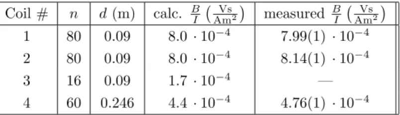
Four different pairs of magnetic-field coils in Helmholz configuration can be used to apply homogenous magnetic fields to the Rb sample; they are labelled 1 to 4. Coils #1 to #3 are aligned collinear with the laser beam (alongzdirection), while coil #4 is aligned transversal to the laser beam (alongxdirection).

The latter may be used for compensation of the vertical component of the Earth’s and other stray magnetic fields. Specifications of the magnetic field coils are listed in Tab.1. Dedicated constant-current power supplies may be used to adjust corresponding field strengths. Use 3.5 mm cables to connect the coils to the power supplies. Further, you may apply variable (longitudinal) magnetic fields via additional coils #5 in your experiments. Each #5 coil hasn= 5 windings, is mounted directly onto the glass cell, and can be connected with a BNC cable.

You may use a radio-frequency (RF) generator to apply RF radiation to the Rb sample via a RF emitter mounted directly onto the glass cell. To control the broadcasting power you can vary the corresponding control voltage UB; maximum output power is set with UB = 30 V. A coarse and fine dial adjust the

(6)

Coil # n d(m) calc. ^B_I _Am^Vs2

measured ^B_I _Am^Vs2

1 80 0.09 8.0 ·10⁻⁴ 7.99(1) ·10⁻⁴ 2 80 0.09 8.0 ·10⁻⁴ 8.14(1) ·10⁻⁴

3 16 0.09 1.7 ·10⁻⁴ —

4 60 0.246 4.4 ·10⁻⁴ 4.76(1) ·10⁻⁴

Table 1: Calculated and measured B/I of the magnetic-field coils #1-#4 with nwindings and inner diameter d.

output frequency and you may use the oscilloscope or a counter to measure the set frequency.

3 Measurement Procedures

3.1 Characterisation of the laser diode

Characterise the relative laser frequency variation for variable diode laser temperatures and drive currents using the etalon.

Instructions:

Turn on the temperature controller and the diode current controller of the diode laser. The laser system needs some time to thermalise (within the laboratory environment) before it’s output wavelength (and power) is sufficiently stable for your measurements. Turn on/off the laser emission by switching the output of the diode controller. You may need to adjust the diode temperature around '34.6^◦C and diode current until the output wavelength is close to the Rb D1 line (fluorescence light may be seen with a mobile phone camera).

You may use the PD amplifier with gain setting 40 dB. When optimising the beam bath use the DC- output for a signal proportional to the light power entering the PD. When data taking you may use the AC-output as this signal has a larger bandwidth. Attach the 9V battery to bias the PD for maximum bandwidth.

Remove the glass cell from the beam path and put in the etalon. Note, make sure the etalon is adjusted such that the laser beam enters orthogonal to it’s surface. Modulate the diode current with a sawtooth signal with constant offset current and constant temperature setting. Check the quality of your modulation signal on the oscilloscope and choose a range for your measurements where the voltage variation is most linear. Optimise the beam path by increasing the etalon transmission signal on the PD. Take calibration measurements of the laser frequency (wavelength) variation as a function of temperature and diode current. Vary only one parameter in a measurement sequence and avoid mode jumps during your sequences. However, you should record representative signals indicating mode jumps, in order to present and discuss this systematic effect in your final analysis.

3.2 Spectroscopy of the hyperfine structure

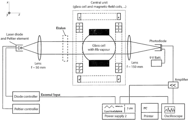
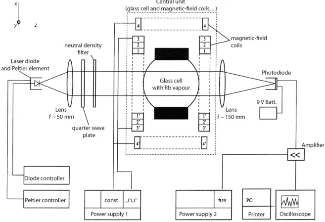
Perform absorption spectroscopy of the ²S_1/2 to ²P_1/2 transition of⁸⁵Rb and⁸⁷Rb and determine the underlying hyperfine structure, cp. Fig.1. In Table2, we list literature values of relevant hyperfine constants. A schematic of the experimental setup is shown in Fig.2.

HFS const. A ⁸⁵Rb (I = 5/2) ⁸⁷Rb (I = 3/2)

2S_1/2 4.185µeV 14.13µeV

2P_1/2 0.499µeV 1.692µeV

Table 2: Hyperfine constants Aof the ²S_1/2 and²P_1/2 levels of Rb [Co77].

(7)

Figure 2: Schematic of the experimental setup for the absorption spectroscopy of⁸⁵Rb und⁸⁷Rb.

Remove the central unit and insert the etalon to perform calibration measurements of the relative laser frequency variation. Figure adapted from [Ba97].

Instructions:

1. Put the glass cell (central unit) into the beam path (without the etalon). Modulate the laser frequency by applying a sawtooth signal to the diode current with a peak voltage of about 100 mV at fixed diode temperature of ' 34.6^◦C. Optimise diode laser settings to record the entire D1- absorption spectrum. Use variable frequencies and different slopes of the modulation signal to study systematic variations of the absorption line shapes. We recommend that you increase the absorption signal by increasing the partial pressure of Rb in the cell.

2. For each measurements sequence you need calibration measurements of the relative laser frequency tuning, in order to analyse your spectra. Use the etalon for these calibrations, while the central unit is removed.

3. Identify individual hyperfine transitions by applying appropriate selections rules and determine the hyperfine constantsA of the²S_1/2and²P_1/2 levels from your spectra.

3.3 Double-resonance experiments

Measurement of the nuclear spin I of both Rb isotopes by optical pumping and RF radiation tuned to double-resonance. Further, the transversal and longitudinal component of the stray magnetic field are to be determined.

• Generation of circular polarised light

• Detection of the absorption signal during the resonant irradiation of laser light and RF radiation

• Compensation of the vertical component of the stray magnetic field

(8)

• Measurement and compensation of the longitudinal component of stray magnetic fields

• Measurement of the nuclear spinI of⁸⁵Rb and ⁸⁷Rb

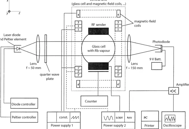
Figure3sketches the setup for the double-resonance experiments. The magnetic field generated by coil

#1 causes a splitting of the magnetic sub-levels. The splitting is illustrated in Fig.1 and, in the case,

Figure 3: Setup for the measurement of the nuclear spin of both Rb isotopes via the double- resonance method: The setup is extend with a quarter wave plate for the generation of circular polarised light. The radio-frequency emitter is mounted directly on the glass cell. It’s frequency can be tuned via the potentiometers on the central unit, its amplitude is adjusted via the power supply.

The frequency can be checked at the monitor output using a frequency counter or an oscilloscope.

The constant magnetic field are applied via coil #1 and #4. The additional oscillating magnetic field is applied via coil #2. Figure adapted from [Ba97].

of low magnetic fields. Here, the level splitting is approximately equidistant and can be sufficiently described by the Zeeman effect. The energy splitting of neighbouring magnetic-sub states (∆mF = 1) in Rb (in the ground state) is given by:

∆E_B= µBB

I+ 1/2. (1)

Here, I denotes the nuclear spin of each isotope, B is the external magnetic field strength, and µB

is the Bohr magneton. At room temperatures the ground state levels are (almost) equally populated.

Due to the optical pumping, there is a significant deviation of the occupation numbers compared to the equilibrium state. Irradiation of resonant circular polarised light (e.g., σ⁺ light) prepares the ground state|F =max, mF =±Fi. Ideally, all atoms are pumped into this stretched state. In this case, light is fully transmitted and the PD detects maximal intensity. The RF radiation redistributes population between the magnetic-sub levels with maximal rate when ∆E_B =hν_RF, with the RF frequencyν_RF [cp.

Eq. (1)]. In turn, absorption of laser light increases again and the PD detects minimal intensity.

(9)

Instructions:

1. Laser is driven at fixed temperature and current; circular polarised light is produced with a quarter wave plate; the orientation of the wave plate is checked with the help of a linear polariser for coarse tuning. For fine tuning you optimise the double-resonance signal.

2. Choose the laser wavelength such that optical pumping occurs and use a sinusoidal modulation of the current through coil #2 withlargeamplitude to find the necessary magnetic-field range. In the measurements you may choose smaller amplitudes. The RF is applied with fixed ν_RF '500 kHz andUB'10 V. Optimise the laser diode current for maximal absorption; find two current settings (at fixed laser temperature), one for each isotope.

3. The laser is driven with the settings determined above. The current of coil #1 is chosen in a way that you get equidistant absorption peaks with twice the frequency of the modulation of the magnetic field¹. Note, that the oscilloscope records the applied voltage and not the current of coil

#2; take the corresponding phase shift into account.

4. Coil #4 is used to compensate the vertical component of the stray magnetic fields: The current is tuned, such that the absorptions is maximal (check applied polarity). The corresponding magnetic field can be calculated from the characteristics of the coil (see Tab.1) and the applied current.

Keep the vertical compensation for the following measurements.

5. When changing the polarity of the current through coil #1, you need to adjust the current value, to get again equidistant absorption peaks. The difference in the current values between both configurations enables us to determine the longitudinal component of the stray magnetic field.

6. When the transversal component of the stray magnetic field is near compensated, you can calcu- late the nuclear spin of the Rubidium isotopes at double resonance and equidistant absorptions according to

I= µ_BB h νRF

−1

2, (2)

taking the longitudinal component of the total magnetic field into account.

3.4 Spin precession

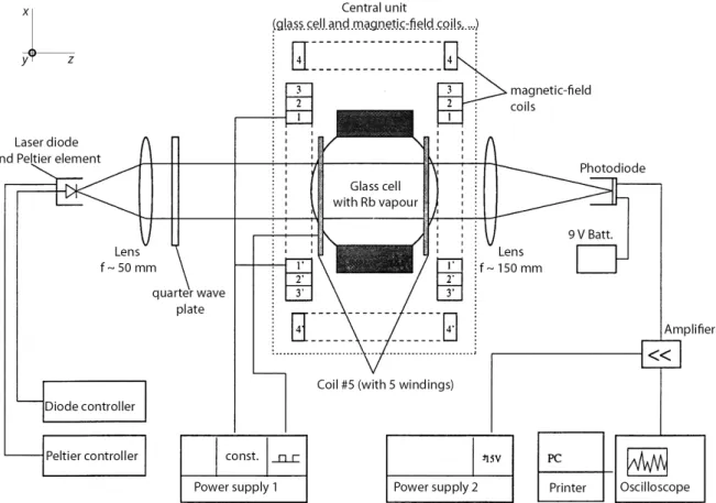
Measurement ofweak magnetic fields by observation of the spin precession. Figure4sketches the setup to determine the vertical component of the stray magnetic field by the observation of spin precession.

The resonant, circular polarised laser beam polarises the Rb along the external magnetic field (sum of stray and applied magnetic fields). When turning off (on) the applied field fast enough (faster than the precession time in the stray magnetic field), the polarisation of the Rb ensemble can not follow the fast changing magnetic field and remains stationary. In absence of the field generated by the coils, the ensemble experiences a torsional moment due to the transversal component of the stray magnetic field and precesses with frequency:

ωL= gFµB

h Bstray,trans. (3)

The polarisation vector follows this precession and the Rb changes with each period from a state of maximum transparency in z-direction into a state of maximum absorption., i.e., the intensity of the transmitted light is a function of time. We can determine the transversal component of the stray magnetic field by the measuring the frequencyνosz of the absorption signal:

BEarth,trans= h gFµB

νosz. (4)

1If there is no absorption, you have to change the diode current, until double-resonance occurs. Optical pumping occurs only in a small region of diode current and laser temperature.

(10)

Figure 4: Setup for the spin precession measurements. The additional coil #5 generates the variable longitudinal magnetic field. The longitudinal components of the stray magnetic field is compensated with coil #1 and its transversal component is compensated with coil #4. Figure adapted from [Ba97].

Instructions:

1. Compensation of the longitudinal component of the stray magnetic field by applying a current to coil #1. It’s current is known from the double-resonance experiment, while it’s transversal component remains uncompensated.

2. The current of coil #5 is periodically switched on and off (choose a rectangular-puls sequence with DC-offset). This coil has a low inductivity and, so far, best results are produced with the ”instec”

function generator. Averaging the signal (with the oscilloscope) will increase the signal to noise ratio, but requires a stable trigger signal.

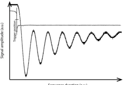
3. With a time resolution of 5µs/div at the oscilloscope, one can observe the spin precession after the falling edge of the magnetic field. We show in Fig.5 a typical trace of the spin-precession signal triggered by the magnetic-field inversion.

4. The transversal magnetic field can be calculated from the frequency of the spin precession. When tuning the current of coil #4 and rotating the experimental table, one may reduce the transversal component of the stray magnetic field. You need to record the spin precession for each parameter setting and compare the quantities of the calculated and measured magnetic fields.

3.5 Relaxation time

Measurement of the relaxation time of the pumped ensembles with the method of Dehmelt (3.5.1) with inversion of the magnetic field and with the method of Franzen (3.5.2) via relaxation in thedark, when

(11)

Figure 5: Illustration of a spin-precession signal of a Rb isotope (black) and of a signal indicating the magnetic-field inversion (grey). Here, the transversal stray-magnetic fields are compensated.

Further, the trigger position is shown and labelled.

the optical pumping light is turned off.

While the optical pumping polarises the Rb any relaxation mechanism acts against the pumping process and depolarises the atoms: When the pumping light is turned off, the polarisation decays. This decay is described by an exponential function with characteristic relaxation timeTR. During the illumination of the ensemble with pumping light, relaxation and pumping process compete against each other and the relevant time constantτ (orientation time) is given by:

1 τ = 1

TP

+ 1 TR

. (5)

Here the pumping time is denoted byT_P and is inverse proportional to the pump light intensityI_light: T_P ∝ 1

Ilight

. (6)

There are two relevant relaxation processes: Rb atoms colliding with the glass cell or with buffer gas.

Further, we only consider the first: When assuming that the polarisation of Rb atoms is completely lost during a single collision with the glass cell, we can estimate the relaxation time from the diffusion rate 1/T_Din the given spherical geometry of the glass cell [Co77]:

1 TD

=D0p0

p

2π

d ²

. (7)

In this equation,dis the diameter of the cell,pdenotes the pressure in the cell, andD₀ is the diffusions coefficient of Rb in a buffer gas with constant pressurep0(literature values listed in Tab.3).

3.5.1 Dehmelt’s method: Inversion of the magnetic field

• Time-resolved observation of the absorption signal of the pumped ensemble after flipping the direction of the applied magnetic field

• Determination of the orientation time τ for different light intensities

• Extract the relaxation timeTRand compare it to calculated values

Figure6sketches the relevant experimental setup. Optically pumped Rb is polarised along the magnetic

(12)

Buffer gas D0[cm²s⁻¹]

He 0,7

Ne 0,5

Ar 0,4

Kr 0,16

Xe 0,13

Table 3: Diffusions coefficients D₀ for Rb in buffer gas at constant pressurep₀= 101.3kPa

Figure 6: Experimental setup for determination ofT_Rwith the method of inverting magnetic-field introduced by Dehmelt. Figure adapted from [Ba97].

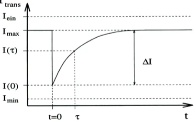
field by the polarised laser light. When at t = 0 the direction of the applied magnetic field is flipped abruptly, the Rb is pumped into the opposite stretched state within TP. For example, if most of the Rb is prepared in |F = 2, mF = 2i prior to the flipping of the magnetic field, it gets subsequently pumped into |F = 2, m_F =−2i². Due to the pumping process, the transmission of light through the cell increases exponentially with the orientation timeτ, cp. Fig.7. Whileτ is defined as the duration at which 1−1/e= 63.2 % of the maximal transmission is reached. From measurements taken with variable pump-light intensity, we can determine the relaxation timeTR[De57].

Instructions:

1. Choose laser settings such that it addresses both Rb isotopes³.

2. Coil #3 is used to generate a longitudinal oscillating magnetic field, while coil #4 is used to compensate the vertical component of stray magnetic fields.

2This example is given for⁸⁷Rb.

3It maybe that the settings need to be (re-) adjusted during the measurement

(13)

Figure 7: Illustration of the transmission signal during a measurement of the orientation dura- tionτ. Figure adapted from [Ba97].

3. The orientation timeτ is measured for variable pump-light intensity using different neutral-density filters. You should take calibration measurements of the transmission through the neutral-density filters. Further, we recommend that you increase the absorption signal by increasing the partial pressure of Rb in the cell.

4. Plot your results for 1/τ as a function of light intensity and determineTR. 3.5.2 Franzen’s method: Relaxation in the dark

• Time-resolved observation of the absorption signal after switching off/on the pump light

• Determination of the absorption signal for different durations in the dark ∆t

• Superposition of the absorption signals for different ∆t and determination of the time of relax- ationTR.

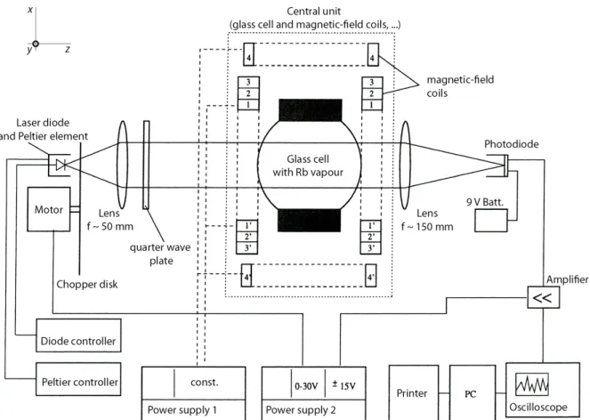
Figure8illustrates the required experimental setup. When the pump light is interrupted by the chopper disk (driven at variable speed), the polarised Rb relaxes until the light is unblocked and it can re-pump the Rb. The relaxation time TR can be determined from the analysis of the time-resolved absorption signals taken at variable durations in the dark ∆t (chopper speeds). Figure9 shows the shape of the absorption signal as a function of sequence durationt.

For ∆t T_R, the system is able to fully relax in the dark, i.e., a uniform distribution of the level population is restored, and the repumping starts from maximal absorption: Imax−Imin. The initial transmitted intensity (absorption level) as function of ∆tis described by:

I(∆t) =Imin+ (Imax−Imin) exp

−∆t T_R

. (8)

You can use this relation to determine the relaxation timeT_R[Ba97,NH,Co77].

Instructions:

• The laser is periodically blocked by the chopper disk driven at variable rotation speed, while the laser wavelength is adjusted for maximal absorption. We recommend that you increase the absorption signal by increasing the partial pressure of Rb in the cell.

• Record time-resolved absorption signals for different ∆t

• Determination of TRfrom a model fit of Eq.8to your data.

• Compare this result with your result for T_Rfrom Dehmelt’s method and discuss systematic differ- ences of both methods.

(14)

Figure 8: Experimental setup for the measurement with Franzen’s method for the determination of the time of relaxation. Figure adapted from [Ba97].

Figure 9: Illustration of the transmission signal expected during the measurements following a relaxation in the dark (Franzen’s method).

References

[Ba97] Baur, C.: Optisches Pumpen mit Laserdioden, Staatsexamensarbeit, Universit¨at Freiburg, 1997

(15)

[Co77] Corney, A.: Atomic And Laser Spectroscopy, Oxford University Press, 1977

[NH] Nagel, M.; Haworth, F.E.: Advanced Laboratory Experiments on Optical Pumping of Rubidium Atoms-Part II, Free Precission, American Journal of Physics, Vol. 34, 559 (1966)

[Fr59] Franzen, W.: Spin Relaxation of Optically Aligned Rubidium Vapour, Phys.Rev.115, 850 (1959) [Ha72] Happer, W.: Optical Pumping, Rev. mod. Phvs 44, 169 (1972)

[De57] Dehmelt, H.G.: Slow Spin Relaxation of Optically Polarized Sodium Atoms, Phys. Rev. 105, 1487 (1957)

[Ko96] Kohlrausch, F.: Praktische Physik, Teubner Verlag, 24. Auflage, 1996