Who Gets The Schools?

(1)

Who Gets The Schools?

Stefan Leiderer

Political Targeting of Economic

and Social Infrastructure Provision

in Zambia

(2)

(3)

Political targeting of economic and social infrastructure provision in Zambia

Stefan Leiderer

Bonn 2014

(4)

Die Deutsche Nationalbibliothek verzeichnet diese Publikation in der Deutschen Nationalbibliografie;

detaillierte bibliografische Daten sind im Internet über http://dnb.d-nb.de abrufbar.

The Deutsche Nationalbibliothek lists this publication in the Deutsche Nationalbibliografie; detailed bibliographic data is available at http://dnb.d-nb.de.

ISBN 978-3-88985-652-4

Stefan Leiderer, Department I: Bi- and Multilateral Development Policy, German Development Institute / Deutsches Institut für Entwicklungspolitik (DIE)

E-mail: Stefan.Leiderer@die-gdi.de

 +49 (0)228 94927-0

+49 (0)228 94927-130 E-mail: die@die-gdi.de www.die-gdi.de

(5)

Niño-Zarazúa, Armin von Schiller and Eva Terberger for extremely valuable comments and suggestions. I also thank Dina Elsayed and Melanie Mirsch for excellent research assistance.

All remaining errors are my own.

Bonn, August 2014 Stefan Leiderer

(6)

(7)

nance in developing countries. Its main methodological interest is to demonstrate the usability of household-level data to study political economy features of public finances in developing countries that commonly escape empirical scrutiny due to poor data availability. The immedi- ate empirical interest is in testing whether there is evidence for or against either of two competing models of political targeting of public sector spending in Zambia: the swing-voter versus the core-voter model, the proposition being that in “typical” neo-patrimonial regimes in sub- Saharan Africa, the core-voter model should prevail. I use data from Zambia’s Living Condi- tions Monitoring Survey (LCMS) to investigate whether there is evidence that the ruling party in Zambia followed political motives in targeting public infrastructure spending at the turn of the millennium. I find strong and robust evidence for the core-voter model applying to social infrastructure provision in Zambia. The findings suggest that it is primarily the construction of new health and education facilities that is affected by political targeting, whereas there is no strong evidence for such targeting for the improvement and rehabilitation of existing infrastructure. For the roads sector, the evidence is less conclusive: although the estimates show the same pattern as in health and education, they are not as robust to modifications in the econometric specification.

(8)

(9)

Abbreviations

1 Introduction: political targeting of public expenditure in developing countries 1 1.1 Public financial management and the concept of neopatrimonialism 1

1.2 Who’s the target? Swing voters versus core voters 1

1.3 The difficult empirics of the political economy of public finance in developing

countries 3

2 Empirical approach 6

2.1 Using household survey data to track political targeting in Zambia 6

2.2 Empirical question and main variables 6

2.2.1 Choice of dependent variable: proxying public sector investment 7 2.2.2 Main explanatory variables: identifying swing and core voters 9

2.2.3 Control variables 11

3 Econometric specification and empirical findings 12

3.1 Electoral success and infrastructure provision 12

3.2 Urban and rural infrastructure 18

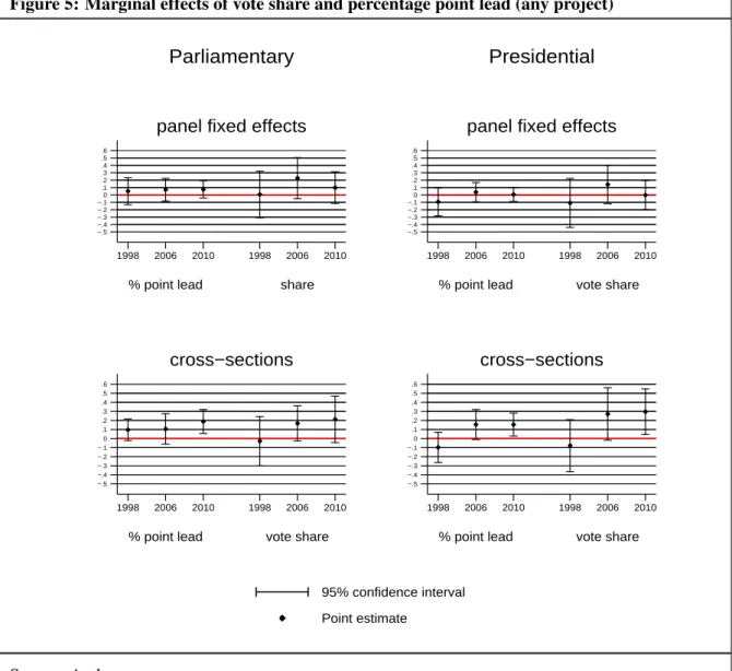
3.3 Parliamentary or presidential elections? 20

3.4 Rehabilitation and improvement versus construction 22

3.5 Threshold effects 29

4 Addressing possible sources of bias 32

4.1 Reverse causality 32

4.2 Measurement error 34

4.3 Reporting error 35

4.4 Omitted variables and selection bias 40

5 Conclusions 45

Bibliography 47

(10)

A Zambia – a showcase of neopatrimonialism 53

A.1 Recent political history of Zambia 53

A.2 Fiscal centralism in Zambia 55

B Data sources 56

B.1 The Zambia Living Conditions Monitoring Survey 56

B.2 Census data 61

B.3 Election data 62

C Description and rationale of control variables 63

D Regression results 67

E Marginal effects plots 105

F Marginal probability plots 107

(11)

2 Vote margins and infrastructure provision: panel regression results 16 3 Number of constituencies won by MMD or opposition by district type 19 4 Vote shares and infrastructure improvement or construction: presidential elections 24

5 40% MMD strongholds by district type 29

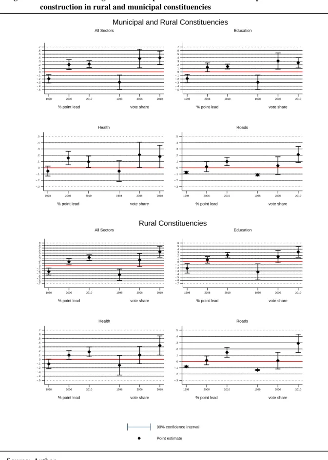
6 Presidential strongholds and infrastructure construction: rural constituencies 31

7 Determinants of presidential electoral success 33

8 Infrastructure construction per SEA: 10% household share threshold 36 9 Probit average marginal effects presidential vote share and 40% strongholds 38 10 Entropy balancing, 2006 reporting period (rural constituencies) 42 11 Entropy balancing, 2010 reporting period (rural constituencies) 42 12 Probit average marginal effects for presidential 40% strongholds after entropy

balancing (construction, rural constituencies) 44

Figures

1 Constituency vote shares for MMD in presidential and parliamentary elections 10 2 Partial effects of vote margin on any type of infrastructure project 17

3 Partial effects of vote margins in cross-sections 18

4 Panel partial effects of vote margins in rural and municipal constituencies 20 5 Marginal effects of vote share and percentage point lead (any project) 22 6 Cross-section marginal effects of presidential vote share and % point lead on

construction in rural and municipal constituencies 28

7 Marginal probability of households reporting construction in 2010 (at sample means) 40

(12)

B.1 Poverty incidence by province 57 B.2 Grand mean constituency average reported distances to nearest transport, health,

and education facility by district type 58

B.3 Mean %-share of households per constituency reporting road projects 60 B.4 Mean %-share of households per constituency reporting health projects 60 B.5 Mean %-share of households per constituency reporting education projects 60 B.6 Mean %-share of households per constituency reporting any project 60 B.7 Number of constituencies dominated by language groups (≥30%) per province 61 D.1 Vote margins and infrastructure provision: cross-section results 67 D.2 Vote margins and infrastructure provision: rural and municipal constituencies (panel) 68 D.3 Vote margins and infrastructure provision: rural constituencies (panel) 69 D.4 Vote margins and infrastructure provision: rural and municipal constituencies

(cross-sections) 70

D.5 Vote margins and infrastructure provision: rural constituencies (cross-sections) 71 D.6 Vote shares and infrastructure provision: all constituencies (panel) 72 D.7 Vote lead and infrastructure provision: all constituencies (panel) 73 D.8 Vote shares and infrastructure provision: cross-section, any project 74 D.9 Vote lead and infrastructure provision: cross-section, any project 75 D.10 Presidential lead and infrastructure improvement or construction (cross-sections) 76 D.11 Parliamentary vote share and infrastructure improvement or construction

(cross-sections) 77

D.12 Parliamentary lead and infrastructure improvement or construction (cross-sections) 78 D.13 Presidential vote share and infrastructure improvement and construction (panel) 79 D.14 Presidential vote lead and infrastructure improvement and construction (panel) 80 D.15 Parliamentary vote share and infrastructure improvement and construction (panel) 81 D.16 Parliamentary lead and infrastructure improvement and construction (panel) 82 D.17 Presidential vote share and road infrastructure provision 83 D.18 Presidential vote lead and road infrastructure provision 84 D.19 Presidential vote share and health infrastructure provision 85 D.20 Presidential vote lead and health infrastructure provision 86

(13)

D.23 Presidential vote share and infrastructure improvement or construction: municipal

and rural constituencies 89

D.24 Presidential lead and infrastructure improvement or construction: municipal and

rural constituencies 90

D.25 Presidential vote share and infrastructure improvement or construction:

D.26 Presidential lead and infrastructure improvement or construction: rural

constituencies 92

D.27 Presidential vote share and infrastructure improvement and construction: rural and

municipal constituencies 93

D.28 Presidential vote share and infrastructure improvement and construction: rural

constituencies 94

D.29 Presidential lead and infrastructure improvement and construction: rural and

municipal constituencies 95

D.30 Presidential lead and infrastructure improvement and construction:

D.31 Vote shares and infrastructure construction: presidential elections, 1998 LCMS 97 D.32 Vote shares and infrastructure construction: presidential elections, 2006 LCMS 98 D.33 Presidential vote share and infrastructure construction: 2010 LCMS 99 D.34 Presidential vote share and infrastructure construction: 2008 elections,

2010 LCMS 100

D.35 Probit average marginal effects by sector, 2006 101

D.36 Probit average marginal effects by sector, 2006: rural constituencies 102

D.37 Probit average marginal effects by sector, 2010 103

D.38 Probit average marginal effects by sector, 2010: rural constituencies 104

Figures in Appendix

E.1 Cross-section partial effects of vote margins for rural and municipal constituencies 105 E.2 Panel fixed effects of presidential vote share and % point lead on construction

in rural and municipal constituencies 106

F.1 Marginal probability of households reporting construction in 2010 (at sample

means), rural constituencies 107

(14)

(15)

AfDB African Development Bank ATE Average Treatment Effect

ATT Average Treatment effect on the Treated (ATT) CDF Constituency Development Fund

CPD Cox-Pesaran-Deaton test

CSO Central Statistical Office of the Republic of Zambia DIP Decentralization Implementation Plan

ECZ Electoral Commission of Zambia

EU–EOM European Union Election Observation Mission FDD Forum for Democracy and Development GMM Generalised Method of Moments LCMS Living Conditions Monitoring Survey LSMS Living Standards Measurement Study MMD Movement for Multi-Party Democracy MoFNP Ministry of Finance and National Planning MoLGH Ministry of Local Government and Housing MP Member of Parliament

NDC National Democratic Congress NDP National Development Plan

OECD–DAC Organisation for Economic Co-operation and Development – Development Assistance Committee

OLS Ordinary Least Squares

PF Patriotic Front

PFM Public Financial Management SEA Standard Enumeration Area UDA United Democratic Alliance

UNIP United National Independence Party UPND United Party for National Development ZCTU Zambia Congress of Trade Unions

(16)

(17)

1 Introduction: political targeting of public expenditure in developing countries 1.1 Public financial management and the concept of neopatrimonialism

Over the past 20 years or so, there has been an enormous increase of interest in public finances in developing countries. To a good extent, this interest is driven by Western aid agencies’

and researchers’ concerns about the effectiveness of development aid and the fiduciary risks associated with channelling aid resources directly through recipient governments’ own public financial management (PFM) systems.

This concern has resulted in a vast amount of reports and analytical studies on the performance of PFM systems and the political determinants of public spending in developing countries, above all in sub-Saharan Africa (de Renzio / Andrews / Mills 2010, 40). One of the central tenets of this body of – mostly “grey” – literature is that PFM systems in sub-Saharan Africa are hampered by characteristic features of the African state that lead to the inefficient use of public resources. The ensemble of these features is commonly subsumed under the concept of

“neopatrimonialism”, which is described as being characterised by the concentration of power in the hands of a small elite, particularly the head of state; few effective checks-and-balance mechanisms or horizontal and vertical division of power; the capture of public resources by these elites to maintain extended clientelistic networks and patronage systems; and the super- seding (or hybridisation) of formal institutions and processes in the public administration by informal and personalised institutions, rules and relations (Bratton / van de Walle 1994; Erd- mann / Simutanyi 2003; van de Walle 2001).

Although the general assessment of the negative impact of neopatrimonial regimes on the performance of PFM systems appears to be widely shared by researchers as well as aid practitioners, it proves remarkably difficult to test these claims empirically and assess the true extent to which neopatrimonialism affects the efficient use of public finances in developing countries. This paper demonstrates the usability of household survey data as a – so far under-exploited – source of information to study one key dimension of allocative efficiency in neopatrimonial regimes: the extent and nature of political targeting of public infrastructure investment across electoral constituencies.

1.2 Who’s the target? Swing voters versus core voters

There exists a relatively large body of economic literature on the political economy of public spending in modern democracies. Much of this literature is concerned with empirically testing the central tenet of Downs’ seminalEconomic Theory of Democracy(Downs 1957) that “polit- ical behaviour in a democracy can be understood as a rational effort to maximize the prospects of electoral success” (Wright 1974, 30).

One important strand within this research, building on early work such as Nordhaus (1975), MaRae (1977), Hibbs (1977) and Tufte (1978), is concerned with the existence of political budget cycles, trying to explain how governments use expansionary fiscal and monetary policy in the run-up to elections in order to increase the chances of being re-elected (Blaydes 2008, 1;

Shi / Svensson 2006, 1368).¹

1 Until recently, empirical studies of political budget cycles focussed mostly on advanced industrial countries and found only inconclusive evidence of the existence of such cycles (Blaydes 2008; Shi / Svensson 2006).

(18)

A related but somewhat differently focussed strand of research is concerned not with the timing of government spending but with its distribution between social groups or across geographic and administrative entities. Two main competing theories exist of how politics may determine the allocation of public funds across beneficiaries: the swing-voter model of distributive politics (Lindbeck / Weibull 1987; Dixit / Londregan 1996), which argues that incumbents target public expenditure to win over undecided voters or buy back opposition voters with no strong political partisanship; and the core-voter model (Cox / McCubbins 1986), which posits that government spending is predominantly used to reward loyal constituencies and political strongholds.² Which of these two competing models applies in real-world political processes is an empirical question that, to date, has not been conclusively answered. Similar to research on spending cycles, until recently most empirical work on politically motivated distribution of public spending focussed on OECD countries.³ In what seems to be a majority of studies, authors find evidence that governments in rich countries use public spending to enhance their re-election probabilities by targeting swing voters and constituencies. This is true for well-studied federal spending under the “New Deal” in the United States, of which a disproportionate share targeted swing states (Couch / Shughart 1998), but also for expenditure programmes in countries such as Sweden, where, for instance, Dahlberg and Johansson (2002) find strong evidence for the swing-voter theorem in the distribution of intergovernmental “ecological” grants.

However, these findings are not undisputed, and a number of studies find evidence instead in support of the core-voter theorem of Cox and McCubbins. Levitt and Snyder (1995), for instance, find that federal outlays in districts in the United States in the second half of the 1980s were positively correlated with the number of democratic voters. Others, again, find evidence for governments to “mix” between the two models, e.g. Milligan and Smart (2005), who find the allocation of regional grants in Canada to be targeting both swing districts and districts represented by a member of the ruling party.

There are good reasons why indeed both theorems might be relevant in practice, depending on the particular context in which governments make their spending decisions. Evidently, the specifics of a country’s electoral system and its concrete political constellation at a particular point in time can be expected to make a difference for how governments attempt to put public spending to use in order to ensure staying in power.⁴

Yet, various authors argue that it is not only the electoral system, but also a country’s broader institutional set-up that ultimately determines whether a government favours swing or core vot-

Newer research seems to confirm the existence of electoral budget cycles (e.g. Persson / Tabellini 2003), but also finds strong indications that the nature of such cycles may differ fundamentally between developed and developing countries (Shi / Svensson 2006).

2 Ansolabehere and Snyder (2006, 549) identify three rationales for core-voter targeting: (i) simple rent- seeking by parties, letting incumbent parties target areas with high concentration of supporters to benefit from government spending; (ii) mobilisation of supporters to vote; (iii) maximisation of credit a party or incumbent receives in case of shared programme responsibilities. Schady (2000, 290) offers two alternative or additional explanations: firstly, incumbents may be risk-averse, and thus more likely to invest in core supporters, whose needs and preferences they understand well, rather than in relatively “unknown” swing voters; secondly, Schady (2000, 290) argues that the fraction of transfers that actually materialise as a benefit to voters may be higher when these are targeted towards core supporters.

3 See, for instance, the extensive work on “New Deal” spending in the 1930s by Arrington (1969), Reading (1973), Wright (1974), Wallis (1984), Anderson and Tollison (1991), Wallis (1998) and others.

4 On the important role electoral systems play for fiscal policy choices, see, for example, Funk and Gathmann (2009).

(19)

ers. This suggests that, in countries with weaker administrative capacities, the core-voter model may prevail, whereas in countries with more efficient public sector institutions, the swing-voter model should apply.⁵

These considerations have led some authors to suggest that – similar to the phenomenon of political budget cycles – there might be systematic differences between the form in which political targeting of public expenditure occurs in rich countries, and how it is applied in developing countries, especially those with neopatrimonial and clientelistic structures.

By and large, most recent literature on the topic (especially that on politics in Africa) seems to follow this line of argument, suggesting that the particularities of developing countries’ politics and institutions favour a core-voter model of public spending rather than a swing-voter model, which appears to be more relevant in advanced democracies.⁶

Yet, even from a neopatrimonial perspective, both models have theoretical merit: clearly, the need to maintain a wide network of loyal “clients” through patronage may be crucial for an incumbent’s political survival in a neopatrimonial system, speaking indeed for the “core-voter”

model to play an important role in the distribution of discretionary spending (van de Walle 2001; Kelsall 2012, 680). At the same time, however, staying in power certainly is a major motivation for an incumbent elite in a “winner-takes-all” political system (Bratton / van de Walle 1994, 465), eventually making it necessary to keep “swing voters” happy as well.⁷ It would seem that, ultimately, this question can only be decided empirically. Yet, to date, there is only limited evidence on the extent of political targeting of public spending in developing countries, and its impact on the efficient allocation of scarce resources (including those provided through government to government aid). The next section reviews some of the empirical literature that directly addresses the question of whether the swing-voter or the core-voter theorem applies in developing countries.

1.3 The difficult empirics of the political economy of public finance in developing countries As discussed in the previous section, most work concerned with empirically investigating the political economy of public finances is focussed on industrialised Western democracies. It is only recently that more work in this strand has been undertaken on cases in developing countries, particularly in Latin America and – to a lesser degree – in sub-Saharan Africa.

The main empirical difficulty in studying questions such as whether the swing-voter or the core-voter theorem applies in practice in neopatrimonial or autocratic systems is the extremely limited availability of reliable data on government expenditure in poor countries.⁸ As Reinikka

5 This point was, in principle, already made in the original argument by Dixit and Londregan (1996), who posited that the incumbents’ decision depends on whether they can collect taxes and distribute benefits more effectively among their supporters than the general population. Where this is the case, incumbents should favour core voters, and swing voters otherwise (Schady 2000, 290).

6 Some authors such as Tavits (2009) argue that targeting core voters is a feasible and rational strategy, not only in developing countries but in advanced democracies as well.

7 In an alternative line of argument, Robinson and Torvik (2009), using Zimbabwe under Robert Mugabe as an example, argue that an incumbent government might have an incentive to repress and disenfranchise swing voters rather than “buy them” in order to maximise the probability of being re-elected.

8 Magaloni (2006), for instance, notes that it took three years to collect data on municipal-level spending in Mexico and that, still, the figures represent only an approximation of government expenditures.

(20)

and Svensson (2004, 679) emphasise, official budget data are typically the only source of information on public spending in low-income countries, and typically these poorly reflect the resources and services actually received by the intended beneficiaries. This is particularly true for sub-Saharan African countries, where fiscal data is usually difficult to obtain and notoriously unreliable. Thus, although there is a good amount of “narrative” work on the impact of neopatrimonial features of government systems on the quality of public financial management,⁹ rigorous empirical analysis of the political economy of public spending in developing countries, in particular in sub-Saharan Africa, is fairly scarce. Existing studies mostly do not examine the total expenditure on public goods and services but rather intergovernmental transfers or specific subsidy programmes for which data are available. What is more, the evidence produced by these studies with regard to the swing-voter / core-voter controversy is somewhat inconclusive.

A number of studies, for instance, investigate the role of patronage politics in Mexico’s PRONASOL poverty-relief programme, e.g. Molinar Horcasitas and Weldon (1994), Hiskey (1999) and Magaloni (2006). Whereas Hiskey (1999) finds evidence for the core-voter theorem in PRONASOL spending, Magaloni (2006), after controlling for simultaneity problems stemming from electoral outcomes being influenced by expenditures from earlier periods, finds evidence for the swing-voter model.

Schady (2000) examines the timing and geographic distribution of expenditures of the Pe- ruvian social fund FONCODES between 1991 and 1995 and finds evidence for expenditure spikes ahead of elections that disproportionally benefited provinces loyal to President Alberto Fujimori, but also provinces that had supported Fujimori at the polls in 1990 but abandoned him in 1993, i.e. a rather specific form of the swing-voter model.

Faust (2012), in turn, analyses resource allocations in Bolivia’s decentralised social fund Fondo de Inversión Productiva y Social and finds little evidence that the allocation scheme was cap- tured by the government or any one of the traditional Bolivian parties. However, there appears to be evidence that municipalities governed by Evo Morales’ anti-system party were signifi- cantly disadvantaged.

For India, Arulampalam et al. (2009) find evidence for an allocation strategy that mixes core- voter and swing-voter elements and under which aligned swing states receive higher transfers than states that are unaligned and non-swing.

In recent years, a number of studies have focussed on post-election targeting of agricultural subsidies, also with inconclusive findings: evidence reported by Mason, Jayne and van de Walle (2013) indicates that fertilizer subsidies in Malawi and Zambia were used to reward areas loyal to the ruling party.¹⁰ In contrast, evidence from a similar study on a comparable programme in Ghana by Banful (2011b) suggests that the fertilizer vouchers were targeted to districts lost by the ruling party in previous presidential elections, and more so in districts lost by a larger margin.

Some related studies look at political economy factors in the distribution of aid projects, although these mostly do not directly address the question of whether the distribution follows a

9 See, for instance, Leiderer et al. (2007), O’Neil (2007), von Soest, Bechle and Korte (2011).

10 Mason, Jayne and van de Walle (2013) test both causal directions, i.e. whether election outcomes affect targeting of subsidised fertilizer, and whether fertilizer subsidies win votes in Zambia. They find no significant effect of subsidies on electoral outcomes.

(21)

core-voter or swing-voter model. Öhler and Nunnenkamp (2013), for instance, use geocoded data on the location of aid projects financed by the World Bank and the African Develop- ment Bank in a sample of 27 recipient countries to assess whether aid targets needy population segments. They find that political leaders manage to direct this aid (and especially physical infrastructure projects) to their home regions, irrespective of regional needs.

In a different approach to circumvent the problem of poor data availability on the geographic distribution of expenditures, Hodler and Raschky (2011) use satellite data on nighttime light intensity and information about the birth places of political leaders to study whether foreign aid is used to fund favouritism. They also find strong evidence that, in countries with weak institutions, local leaders are able to direct aid resources to their birth regions, but not so in countries with sound institutions.¹¹

Briggs (2012) uses data from a large World Bank and bilateral-donor-funded National Elec- trification Project in Ghana that ran from 1993 to 1999 to examine whether the ruling party was able to allocate aid resources according to political criteria. Briggs (2012) finds that the ruling National Democratic Congress (NDC) was able to aim electrification at those regions and constituencies where it had received more votes in previous elections.¹²

In sum, the empirical evidence on the political targeting of public expenditure in developing countries is still thin and mostly inconclusive. More importantly, because of poor data availability, most of the existing evidence is either on ring-fenced aid projects, intergovernmental transfers or very specific government programmes such as agricultural subsidies. Although such programmes can represent a considerable share of the respective sector budgets, they usually account for only a small share of total government expenditure. For instance, the fertilizer subsidy programme investigated by Mason, Jayne and van de Walle (2013) and similar programmes in Zambia accounted for two-thirds of Ministry of Agriculture expenditure between 2003 and 2009. However, total agricultural expenditure (including donor-funded projects) accounted for only 7.4 per cent to 13 per cent of total government expenditure between 2000 and 2008 in Zambia (de Kemp / Faust / Leiderer 2011, 149f). The same applies to intergovernmental fiscal transfers, which usually represent only a minor share of public expenditure in neopatrimonial settings, where discretionary power over the use of resources tends to remain highly centralised.

Moreover, most existing studies investigate the distribution of transfers or subsidies that are relatively easy to target, as they typically involve either cash or in-kind transfers of private goods that are both excludable and rivalrous. It is, however, by no means clear whether findings on the political targeting of such subsidy programmes readily extend to general public expenditure and the provision of public goods and services.¹³ Yet, it is the provision of public goods such as economic and social infrastructure that usually accounts for the lion’s share of government expenditure in developing countries, and that presumably is essential for the economic and social development of these countries.

11 Although, strictly speaking, this is not necessarily evidence for the core-voter theorem, it provides support to the hypothesis that the strength of institutions plays a key role in determining the way in which public expenditure can be politically targeted by incumbent governments.

12 In return, Briggs (2012, 617) finds that electrification projects increased support for the NDC.

13 Diaz-Cayeros and Magaloni (2003, 4) argue that clientelism (i.e. the exchange of state resources for political support (Mason / Jayne / van de Walle 2013, 16)) and the provision of public goods are not contradictory but can coexist, being preferred by both voters and politicians.

(22)

Against this backdrop, this paper contributes to the literature discussed above by investigating whether the distribution of public infrastructure investment in a “typical” neopatrimonial state such as Zambia¹⁴ follows politically motivated patterns, and whether these patterns are in line with either the swing-voter or the core-voter theorem. To circumvent the lack of reliable public expenditure data, this paper proposes the use of information from household survey data to approximate public infrastructure provision.

2 Empirical approach

2.1 Using household survey data to track political targeting in Zambia

Detailed data on public expenditure in sub-Saharan African countries is notoriously scarce and inaccurate. Publicly available sources such as the International Monetary Fund’s Government Finance Statistics report mostly missing values for sub-Sahara African and other developing countries. At the country level, even in those cases where aggregate budget documentation is comparatively comprehensive and transparent, reliable data on the geographic distribution of public expenditure is usually very difficult to extract from budget documents and government financial reports, in particular for sectors that receive significant amounts of off-budget spending, e.g. from international donors. These constraints make sound empirical work on public finances in sub-Saharan Africa extremely difficult, if not often impossible.

At the same time, an increasing number of African countries have well-established databases on household-level living conditions based on regularly conducted Living Standards Measurement Studies (LSMSs). These surveys commonly include information on households’ access to and use of public infrastructure and services.

Beyond contributing new evidence to the swing-voter / core-voter controversy, the main methodological interest of this paper is in demonstrating the usability of such survey data for these types of empirical questions. To do so, I employ data from Zambia’s Living Conditions Monitoring Surveys (LCMSs) to test whether the geographic distribution of public infrastructure provision in Zambia around the turn of the millennium was politically motivated, and if so, which specific strategy the government employed in its political spending.

2.2 Empirical question and main variables

The main empirical question of this paper is whether the geographic distribution of public spending on physical infrastructure in Zambia is politically motivated, in the sense that public investment decisions are shaped by previous electoral outcomes; and – if there is evidence for such politically motivated spending – in which form it occurs.

Formally, the hypothesis underlying this question can be expressed as

I_{c t}^j = f(elec_c,_t₋₁,z_c,^j _t) (1) where the amount of investment I in economic and social infrastructure of type j in a con- stituencycin periodtis a function of the electoral outcome (elec) in that constituency from the

14 See Appendix A for a discussion as to why Zambia lends itself particularly well as a case study to empirically track patronage in public spending in a “typical” neopatrimonial governance system.

(23)

preceding elections and a vector of other variableszthat influence a government’s decision on the amount and geographic distribution of infrastructure investment of type j.¹⁵

Unfortunately, in Zambia, as in most African countries, there is very little detailed – let alone reliable – data on public spending at a disaggregated level, i.e. there is no readily available direct measure ofI_{c t}^j to test this hypothesis underlying Equation 1.¹⁶ However, as the following section explains, more readily available household survey data contains information that can be used as a proxy for public sector investment.¹⁷

2.2.1 Choice of dependent variable: proxying public sector investment

As described in Appendix B, the Zambia LCMS contains different types of household-level information that may be employed to approximate public expenditure at the constituency level.

There are two obvious choices for constructing a proxy variable for physical infrastructure investment from this data, each with its specific advantages and disadvantages.¹⁸

For one, households are asked to report the distance to various types of facilities, including transport, health and basic education facilities. Investment in additional infrastructure in a constituency between two rounds of LCMS surveys should be reflected through a reduction in the average reported distance to the respective type of facility in that constituency, and the average change in distance should thus provide a rough proxy measure for (dis-)investment in public infrastructure at the constituency level.¹⁹

This measure would have the advantage that – by gauging the change in distance to a facility – it takes into account that, in some cases, the government may decide that it is more efficient to improve access to existing facilities by, for instance, building a bridge rather than an additional health or education facility. A disadvantage of this measure – besides the fact that it cannot be constructed for road infrastructure due to missing information in the LCMS – is that it only provides a proxy for the construction of new facilities and disregards investment in improving or rehabilitating existing infrastructure.

The main downside of using changes in average reported distances as proxy measures for investment in public infrastructure, however, is that it relies on aggregate information from dif-

15 This formulation takes into account that the provision of each type of infrastructure such as roads or health and education facilities may each depend on different factors.

16 This not only applies to government spending from the national budget; as in all aid-dependent countries, significant amounts of public spending in Zambia are channelled outside government systems, e.g. by international donor agencies or non-governmental organisations that carry out projects and programmes at various levels and in different sectors in the country. Although the latter does not imply that the central government cannot influence the allocation of these resources, there usually is no unified and publicly available reporting system on this type of expenditure (see, for instance, de Kemp / Faust / Leiderer 2011, 142). What is more, both governments and donors are usually reluctant to publish this kind of information.

17 Appendix B describes the data sources and construction of the main variables.

18 The focus on infrastructure investment rather than general public expenditure is a pragmatic choice. The LCMS does contain information that could arguably be used to construct proxy variables for the provision of general services in some sectors as well, but only with important conceptual difficulties and burdened with empirical challenges such as the need to control for quality. In comparison, the information used to approximate infrastructure investments is much less ambiguous.

19 Because the LCMS does not survey the same households in each round, it is not possible to observe reductions in distance for individual households.

(24)

ferent households in each period, since the LCMS is not a balanced panel but surveys a new sample of households in each round. This may lead to important reporting and measurement errors.

A brief inspection of the averages across all constituencies of this change-in-distance measure for the three periods 1996–1998, 1998–2006 and 2006–2010 (shown in Table 1) suggests that this may indeed be the case: whereas the mean reduction in distance for the two later periods for all three types of facilities is positive, indicating improved access to infrastructure as measured at the national level, there are suspiciously large positive and negative changes between the two points in time. For the 1996–1998 period, the average reduction in distance is negative for health and 0 for education infrastructure, suggesting an overall deterioration of health and stagnation in education infrastructure across the country.²⁰

Table 1: Change in access to facilities 1996–1998, 1998–2006 and 2006–2010^∗

1996-1998 1998-2006 2006-2010

min max mean sd min max mean sd min max mean sd

Transport - - - -21.96 75.24 2.08 11.10 -50.97 19.19 .50 7.07

Health -38.36 .72 -6.48 6.70 -17.87 33.64 1.32 6.66 -28.25 15.89 .39 4.76 Education -13.14 7.94 -.01 2.08 -12.35 15.47 .26 2.61 -4.48 11.31 1.80 1.80

∗Average distance reduction in km per constituency

Source: Author, based on LCMS 1996, 1998, 2006, 2010

Fortunately, an alternative and more direct measure of infrastructure investment is available from the LCMS. In each round, households are asked whether different types of projects have taken place in their community in the period preceding the survey, including construction and improvement / rehabilitation of health and education facilities as well as building and improving different types of roads.²¹ A straightforward way to construct measures for infrastructure investment at the constituency level from this information is to calculate the share of households in each constituency reporting a particular type of infrastructure project.²²

The advantage of basing a (proxy) measure of infrastructure investment on this kind of household reporting is that it records both construction and rehabilitation / improvement of roads and facilities. Thereby, it is possible to account for the fact that in some (e.g. urban) areas where more infrastructure already exists, the rehabilitation and improvement of existing roads,

20 Note that the values given in Table 1 are reduction in distance, i.e. a positive value represents improved access to infrastructure, a negative value stands for a deterioration in access. Especially the large negative minimum values (representing an increase in distance to the nearest facility) cast doubt on the accuracy of this measure and the aggregation across different households in different survey rounds. Evidently, facilities may be abandoned or destroyed and – as anecdotal evidence suggests – it is not uncommon for rural communities’

access to existing infrastructure to be disrupted by rains washing away roads and bridges (Leiderer et al.

2012). However, these occasional events would hardly seem sufficient to explain the large negative measures observed in the data.

21 In the 1998 LCMS, households were asked to report whether projects had taken place during the past five years. In the 2006 and 2010 LCMSs, the reporting period was reduced to the 12 prior months. For details, see Appendix B.1.

22 This approach is similar to the one taken by Terberger et al. (2010), who use the share of households in each of 187 traditional “chief areas” reporting road projects as a measure of the extent to which households in an area benefited from road infrastructure investment in order to assess the impact of roads on poverty and other measures of well-being.

(25)

schools and health posts and clinics may be more relevant than in other areas where construction of new facilities is more relevant.

At the same time, this measure is not a perfect gauge of infrastructure provision at the constituency level either. For one, taking the constituency share of households reporting an infrastructure project obviously involves a large amount of “double-counting” of individual projects, as households located in one area will report on the same roads or facilities constructed or improved in their neighbourhood. This implies that, for any given level of infrastructure investment, one would expect the share of households being aware of that investment to be larger in smaller and more densely populated constituencies than in larger, less populated ones. Con- sequently, there is a need to control for population density when using this measure as a proxy for investments undertaken.²³

Moreover, because the question in the 2006 and 2010 LCMSs records only projects undertaken in the 12 months prior to the survey, it most likely captures only a fraction of the infrastructure projects undertaken since the preceding survey (and the last elections). This would certainly be an important limitation if the objective was to gauge the total amount of public infrastructure investment between surveys. For the empirical question at hand here, however, it should not pose a problem as long as the government discriminates between supporting and opposition constituencies only, with respect to the amount – and not the timing of – infrastructure provision.²⁴

2.2.2 Main explanatory variables: identifying swing and core voters

The main explanatory variable in the model described by Equation 1 is the outcome of elections preceding the respective household survey. It is, however, by no means obvious as to what the appropriate measure for this outcome should be; in particular, whether this measure should be based on the ruling party’s electoral success in parliamentary or presidential elections.

The literature on neopatrimonialism in Africa does not give clear indications in this respect. In principle, one of the key features of neopatrimonial regimes is the concentration of power and resources in the presidency, whereas parliaments in these systems tend to be weak and mostly accountable “upwards” to their party leaders rather than “downwards” to their constituencies (Cammack 2007, 603).²⁵ This wouldprima faciespeak for the outcomes of presidential elections being the relevant main explanatory variable. At the same time, however, political leaders’

reliance on clientelistic networks might mean that an incumbent president in a neopatrimonial system has to use available resources to keep key party members (i.e. members of parliament) content by strengthening their power base and thus increase their chances of being re-elected.

In this case, parliamentary elections might matter more than presidential ones for determining the government’s allocation decisions, even though control over public resources is concen- trated in the president’s hands.

23 There are other reasons too for controlling for population density related to efficiency considerations in the distribution of infrastructure (see Section C).

24 Although it is one of the tenets of some of the literature reviewed in Section 1.3 that politicians tend to time public expenditure in order to increase the probability of being re-elected, there is no particular reason (and no indications from the literature) to suspect that the timing of projects should systematically differ between constituencies that show different degrees of support for the ruling party or candidate.

25 This observation certainly applies to Zambia (see, for instance, de Kemp / Faust / Leiderer 2011, 104).

(26)

From a theoretical point of view, it is thus by no means clear whether the outcomes of presidential or parliamentary elections should be expected to drive allocation decisions in case political targeting takes place. Obviously, both are highly correlated; yet, as shown by plotting the percentage shares received by Zambia’s ruling Movement for Multi-Party Democracy (MMD) in the 1996, 2001 and 2006 presidential elections against those received in parliamentary polls (see Figure 1), this correlation is far from perfect and varies substantially between periods,²⁶ earning this question some closer scrutiny. For the initial steps of the analysis, I therefore examine the role of electoral success of the ruling party in both parliamentary and presidential elections.

Figure 1: Constituency vote shares for MMD in presidential and parliamentary elections

Source: Author, based on data provided by ECZ

Besides this question, there are also different possibilities for how electoral “success” should be defined, in terms of absolute majorities (i.e. the share of votes received in a constituency), or relative majorities (i.e. the margin by which a constituency is won or lost). The “correct”

measure for electoral success will depend on the way in which the government arrives at its decision that a constituency forms part of its own power base and therefore merits dispro- portional infrastructure investment under the core-voter model, or that a constituency is “contested enough” to attract investment under the swing-voter stratagem. Linking to the discussion above, the government’s assessment in this respect might differ, depending on whether it considers parliamentary or presidential electoral outcomes, given the different voting systems in each: presidential elections in Zambia (as in all presidential systems) are decided by the nation- wide majority of votes, whereas parliamentary seats are contested at the constituency level in a first-past-the-post system. Given this fundamental difference of how winners are determined, one would, in principle, expect the government to consider absolute vote shares in presidential elections, and relative majorities in parliamentary elections.

Crucially, however, whether the government considers vote shares or winning (and losing) margins in its allocation decision might depend not only on whether it bases this decision on presidential or parliamentary elections, but also on whether it follows the swing-voter or core-voter stratagem. This is because the government cannot observe individual voters’ preferences to target its infrastructure investment in such a way as to either win over the maximum

26 Pairwise correlation coefficients are: .68 (1996), .94 (2001) and .85 (2006).

(27)

number of swing voters or “reward” the maximum number of its supporters.²⁷ Instead, it has to derive voters’ expected political preferences from constituency electoral outcomes (Schady 2000, 290).

As can be shown, the probability that a randomly selected voter in a constituency will have voted for a particular party is equivalent to the share of the vote for that party in the constituency (Schady 2000, 290; Deacon / Shapiro 1975). In other words, swing voters live in swing constituencies, i.e. voters in highly contested constituencies are more likely to be swing voters than individuals in less contested constituencies. Vice versa, core voters with a strong preference for one party tend to live in constituencies with a high vote share for that party. This implies that if the government wants to benefit mainly its core supporters, then it should target those constituencies where it received the highest vote shares, as these will have the largest share of loyal supporters in the population. Conversely, if it wants to target the maximum number of voters who can be easily swayed to support one party or another, then it should target constituencies with narrow relative majorities, as these can be expected to have the largest share of such swing voters in the population. This, however, will not depend on the absolute share of votes received by the ruling party alone, but also on the distribution of votes among opposition candidates. Thus, if the government wants to win over swing voters, then the margin by which a constituency was won or lost should be the decisive factor. Conversely, if the government wants to use public infrastructure investment to reward its core voters, then it should base its allocation decision on the absolute share of votes received in a constituency.

As the purpose of this empirical analysis is to test these two proposed targeting models against each other, to start with, I take both measures for electoral success into consideration.

2.2.3 Control variables

Evidently, there is a range of confounding factors that may influence the central government’s decisions about where to provide road, health or basic education infrastructure and therefore need to be controlled for. For the main regressions, to control for general deprivation, I include the constituency’s poverty headcount; to control for size effects, a possible rural-urban bias and double counting of projects, the square root of the constituency population, the district population density and dummy variables identifying whether a constituency is located in a municipal or city district (rural districts providing the reference category) are included. To control for sector-specific deprivation, I include the average reported distance to the nearest transport, health and basic education facilities. For geographic factors such as climate, topography and re- moteness, I include province dummies; and as a measure of ethnic group dominance, I include dummies for four of the five largest language groups, indicating whether at least 30 per cent of household heads in a constituency indicate using that language as their primary language.

Additional controls for robustness checks include the distances by road to the national capital and the respective province capital, the percentage share of households belonging to each of the main language groups, and households’ expressed preferences for infrastructure projects to be implemented in their community.

A more detailed description of the rationale for each of these controls is given in Appendix C.

27 In addition, of course, individuals or households located in the same area cannot be excluded from the use of public infrastructure such as roads, health centres or schools constructed in that area.

(28)

3 Econometric specification and empirical findings

The remainder of this paper is concerned with, first, empirically testing whether the general relation suggested by Equation (1) in Section 2.2 applies in Zambia, i.e. whether the geographic distribution of public infrastructure provision is subject to political targeting; and second, exploring the functional form of f, that is, whether such targeting is in agreement with the predictions of either the swing-voter or the core-voter theorem.

As discussed in the previous section, in the absence of detailed and reliable data on government expenditure, I use information from the Zambia Living Conditions Monitoring Survey (LCMS) on households’ reporting of infrastructure projects in their community as a proxy for the public (or publicly sanctioned) provision of economic and social infrastructure. As an initial approach, I take the percentage share of households within each constituency that report at least one infrastructure project (construction or improvement / rehabilitation) in any of the three sectors – roads, health or basic education – in the 1998, 2006 and 2010 LCMSs, respectively, and regress this share on electoral outcomes of the previous parliamentary and presidential elections (held in 1996, 2001 and 2006).²⁸

3.1 Electoral success and infrastructure provision

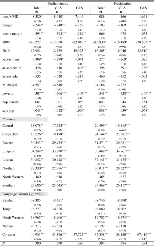
Exploring the evidence for political targeting of infrastructure provision in the data without pre-empting the functional form in which this targeting occurs, requires an econometric specification that can accommodate for both proposed targeting models. Banful (2011b)²⁹ formu- lates such a model (based on relative majorities) by including three main independent variables in the regression: a dummy variable“won” indicating if a constituency was won by the ruling Movement for Multi-Party Democracy (MMD) in elections preceding the relevant LCMS reporting period; a variable“margin”that gives the (absolute) difference in the percentage of votes received by the ruling party’s candidate and by the strongest opposition candidate in that constituency; and an interaction term of these two variables.³⁰ The logic of this specification

28 Note that this is a conservative measure of the number of infrastructure projects undertaken in a community, as every household is counted only once, irrespective of how many different projects it reports. Although this clearly tends to underestimate the amount of infrastructure provided, this choice is made for ease of interpre- tation of the results. The difficulty lies in aggregating the information provided by households on different projects in different sectors. An alternative way to do this would be to simply sum up the percentage shares of households in a constituency reporting improvement and construction projects in each sector, yielding values for the aggregate dependent variable between 0 and 600 (improvement / rehabilitation and construction projects in three sectors), or 300 if construction and improvements are viewed separately. All regressions for aggregate outcome variables reported in this section (including those for construction or improvement / rehabilitation only) were also run with aggregates calculated in this way. The results do not differ substantially and support the findings reported throughout this section (yielding higher coefficients and significant results in some cases), yet coefficients are very difficult to interpret using these specifications.

29 Banful (2011b) studies political targeting of fertilizer subsidies in Ghana. The same specification is used by Mason, Jayne and van de Walle (2013) in their study of fertilizer subsidies in Zambia. Both studies use presidential election outcomes as the main explanatory variables.

30 The MMD was in power continuously from 1991 to 2011 (see Appendix A). However, the vote share that secured a majority for the MMD’s candidate at the constituency level varied substantially between constituencies and years during that period, as did the vote margins in those constituencies won and lost. For presidential elections in 1996, the average share of votes winning the MMD a majority in a constituency (with only 10 constituencies lost) was 70.02 per cent of the cast votes (standard deviation 12.8). The smallest share of cast votes securing a “win” in a constituency was 35.21 per cent, whereas the highest vote share losing the MMD a constituency was 38.11 per cent. The average margin between the MMD’s candidate and the strongest

(29)

is as follows: if electoral outcomes do not affect the government’s allocation decisions, then the coefficients on all three electoral variables (“won”, “margin” and their interaction) are expected be 0. In case infrastructure investment is politically targeted (based on vote margins), then the coefficients on the “margin” variable and its interaction with the “won” dummy should be different from 0. In case the swing-voter model applies, both should be negative, as more contested constituencies receive higher levels of investment than less contested ones. Under the core-voter model, in turn, one would expect a negative coefficient on the “margin” variable and a positive sign on the interaction term, as constituencies receive higher levels of investment when their support for the ruling party is stronger.

Using this specification, I estimate the three available cross-sections (1996, 2001, 2006 elections; 1998, 2006, 2010 LCMSs) jointly in a three-period panel as well as individually for both parliamentary and presidential elections, using any type of infrastructure project (i.e. construction or improvement of roads, health or education facilities) as the dependent variable. To account for the fact that the overall investment volume varies over time, I allow for time-fixed effects.

When choosing the appropriate panel estimator for the described model, one faces a dilemma, however. In order to account for the fact that the dependent variable is censored left at 0 and right at 100 per cent, one would preferably estimate a fractional response or a two-limit tobit model, since a linear estimator might be biased under these circumstances. At the same time, it cannot be ruled out that there might be unobserved constituency characteristics that are correlated with election outcomes. If this were the case, then a random effects estimator would produce biased results, and a fixed effects estimator would seem more appropriate (assuming that the unobserved variables are time-invariant). Unfortunately, there is no parametric fixed effects estimator for models allowing for censoring of the dependent variable. Moreover, many of the included control variables are time-invariant, meaning that their influence on infrastructure provision cannot be identified in a fixed effects model.³¹

There is thus no ideal solution for estimating the repeated cross-sections as a panel. On balance, for this initial analysis, preference is given to the fixed effects model, seeing that the censoring of the dependent variable is of minor importance for the aggregate infrastructure measure,

contender was 53.10 percentage points (51.76 in constituencies won, 1.35 in those lost). In the 2001 (2006) elections, the average share of votes in constituencies carried by the MMD candidate was 44.26 (63.68) per cent with a standard deviation of 9.76 (13.21). The average vote for the MMD candidate in constituencies

“lost” by the MMD was 20.49 (24.00) per cent, with a standard deviation of 9.37 (10.26). The average vote margin in 2001 was 26.69 percentage points (10.67 in those won, 16.02 in those lost by the MMD); in 2006 it was 38.62 percentage points (21.04 in those won, 17.58 in those lost). For parliamentary elections, the equivalent average margin was much more consistent over time, with 36.88 percentage points in 1996 (34.15 in those won, 2.73 in those lost), 23.50 percentage points in 2001 (11.39 in those won, 12.10 in those lost) and 26.71 percentage points in 2006 (14.78 in those won, 12.23 in those lost).

31 Unfortunately, a standard Hausman test to check whether the random effects model is appropriate cannot be applied here, as the test’s requirement that the data cannot be clustered is presumably violated here. A feasible test of the random effects versus the fixed effects model (in a linear model) in this case is the arti- ficial regression approach described by Arellano (1993) and Wooldridge (2002, 290f.), in which a random effects equation is re-estimated, augmented with additional variables consisting of the original regressors transformed into deviations-from-mean form (implemented by the STATA “xtoverid” command). Unlike the Hausman test, the xtoverid procedure extends straightforward to heteroskedastic- and cluster-robust versions.

The null-hypothesis of this test – that the difference in coefficients between the fixed effects and random effects model is not systematic – is not rejected at the conventional levels for either health or education infrastructure, indicating that the random effects model is appropriate for the linear model with clustered standard errors (xtreg) and, by extension, should produce unbiased (and efficient) estimates in the tobit specification.

(30)

and the potential bias in the estimates introduced by ignoring the censoring of the dependent variable (and estimating a linear model) can thus be expected to be less important than the bias caused by the potentially inconsistent random effects estimator.³² At the same time, it is not unlikely that in the relatively small panel data set available for this analysis – with a maximum of 150 observations and only 3 periods – there is insufficient variation in the main variables over time for the fixed effects estimator to produce significant coefficients. Because of this, and in the interest of comparability of panel regression results with those for individual cross- sections, tobit random effects and GLS random effects estimates are also reported throughout the initial steps of this analysis.

The econometric model for the fixed effects panel regression then takes the form share_pro jc,t=α^t⁺µ^c⁺β1wonc,t+β2marginc,t

+β3won×margin_c,t+δ ^zc,t+εc,d,t

(2)

whereshare_pro j_c,tis the share of households in constituencycreporting investment in infrastructure in periodt; αt is the sum of a constant and a time-fixed effect; µc is a constituency- specific effect; wonc,t is a dummy variable with value 1 if constituencyc was carried by the MMD candidate in elections int, and 0 otherwise;marginc,t is the absolute difference of the vote share received by the MMD’s candidate and that of the strongest opposition candidate in constituency cint; zct is a vector of control variables; andεc,d,t is a (district-clustered) error term.³³ As explained in Section 2.2.3, z_ct includes the access (measured by average reported distance) to transport, health and education infrastructure in the previous reporting period as a measure of a constituency’s deprivation in each sector, as well as the constituency’s poverty headcount as a measure of general deprivation. Province dummies are included to account for geographic factors. In addition, in order to control for ethnic group dominance, I include 30 per cent language group share dummy variables.³⁴

32 In fact, for the combined dependent variable that gives the share of households per constituency reporting any kind of infrastructure project, censoring is not a real issue, with only four left-censored cases in 1998, one in 2006 and two in 2010; and three right-censored observations in 1998, none in 2006 and two in 2010. For the more disaggregated infrastructure indicators used in the regressions further down, however, left-censoring is potentially much more relevant: for instance, in 1998, households in 85 constituencies reported no construction of roads, in 47 no construction of health facilities and in 42 no construction of basic schools. In 2006 (2010) the respective numbers are roads: 47 (37), health: 24 (30) and education 17 (17). For rehabilitation and improvement of existing facilities, the number of censored observations in 1998, 2006 and 2010 for roads is: 32, 18, 21; for health: 31, 15, 14; and for education: 12, 3, 6. Right-hand censoring, however, is evidently not of major importance in the data: in 1998 and 2010 there were only three constituencies in which all households report “any improvement”; in 2010 there is one with all households reporting “any construction”.

For the individual sector indicators, there is only one constituency in 2010 in which all households report improvement / rehabilitation of a basic education facility. Taking this into account, all regressions for disaggregated indicators as well as individual cross-sections further down are tobit regressions accounting for left-censoring at 0.

33 Taking into account the fact that groups of constituencies lie within the same districts and that – even though the financial resources at this lowest administrative tier are extremely limited – at least some planning and possibly decision-making takes place at the district level, the estimates may be affected by intra-group correlation of errors. I therefore cluster standard errors at the district level in 72 district clusters.

34 Note that for the dependent variable, i.e. share of households reporting infrastructure investment,t stands either for the LCMS of 1998, 2006 or 2010. For the main explanatory variable, i.e. presidential or parliamentary election outcomes,tstands for the 1996, 2001 and 2006 elections, respectively. Some of the control variables are (taken to be) time-invariant, such as province dummies and ethnic group dominance. For those control variables that measure infrastructure needs or general deprivation, such as distances to transport, health and primary education facilities, or the constituency’s poverty headcount, values are calculated from