Policy Research Working Paper 7473
Households or Locations?
Cities, Catchment Areas and Prosperity in India
Yue Li Martín Rama
East Asia and the Pacific Region Office of the Chief Economist November 2015
WPS7473
Public Disclosure Authorized Public Disclosure Authorized Public Disclosure Authorized Public Disclosure Authorized
Abstract
The Policy Research Working Paper Series disseminates the findings of work in progress to encourage the exchange of ideas about development issues. An objective of the series is to get the findings out quickly, even if the presentations are less than fully polished. The papers carry the names of the authors and should be cited accordingly. The findings, interpretations, and conclusions expressed in this paper are entirely those
Policy Research Working Paper 7473
This paper is a product of the Office of the Chief Economist, East Asia and the Pacific Region. It is part of a larger effort by the World Bank to provide open access to its research and make a contribution to development policy discussions around the world. Policy Research Working Papers are also posted on the Web at http://econ.worldbank.org. The authors may be contacted at yli7@worldbank.org.
Policy makers in developing countries, including India, are increasingly sensitive to the links between spatial transformation and economic development. However, the empirical knowledge available on those links is most often insufficient to guide policy decisions. There is no shortage of case studies on urban agglomerations of different sorts, or of benchmarking exercises for states and districts, but more systematic evidence is scarce. To help address this gap, this paper combines insights from poverty analysis and urban economics, and develops a methodology to assess spatial performance with a high degree of granularity. This methodology is applied to India, where individual house- hold survey records are mapped to “places” (both rural and urban) below the district level. The analysis disentangles the contributions household characteristics and locations make to labor earnings, proxied by nominal household expenditure per capita. The paper shows that one-third of the variation in predicted labor earnings is explained by the locations where households reside and by the interac- tion between these locations and household characteristics
such as education. In parallel, this methodology provides a workable metric to describe spatial productivity patterns across India. The paper shows that there is a gradation of spatial performance across places, rather than a clear rural-urban divide. It also finds that distance matters:
places with higher productivity are close to each other, but
some spread their prosperity over much broader areas than
others. Using the spatial distribution of this metric across
India, the paper further classifies places at below-district
level into four tiers: top locations, their catchment areas,
average locations, and bottom locations. The analysis finds
that some small cities are among the top locations, while
some large cities are not. It also finds that top locations
and their catchment areas include many high-performing
rural places, and are not necessarily more unequal than
average locations. Preliminary analysis reveals that these
top locations and their catchment areas display charac-
teristics that are generally believed to drive agglomeration
economies and contribute to faster productivity growth.
Households or Locations?
Cities, Catchment Areas and Prosperity in India
Yue Li and Martín Rama
Keywords: poverty, labor earnings, location effects, spatial analysis, urbanization, catchment areas.
JEL classification: O18; I32; J31; R12; R23; C21
Yue Li and Martín Rama are with the office of the Chief Economist for South Asia, at the World Bank. The
authors gratefully acknowledge the skillful research assistance provided by Virgilio Galdo and María Florencia
Pinto, and the useful comments and suggestions received from Urmila Chatterjee, Rinku Murgai, Ambar Narayan,
and Mark Roberts. The research was partly funded by the Department for International Development of U.K. as
part of the Sustainable Urban Development Multi-Donor Trust Fund.
1. Introduction
As production diversifies away from agricultural activities into manufacturing and services, the economic landscape evolves too. Urbanization is the most obvious manifestation of this change. But the spatial transformation goes beyond the emergence and growth of cities, as rural areas also densify and the boundaries between urban areas and the countryside become blurred. Policy makers in developing countries are increasingly interested in the implications of this spatial transformation. However, there is limited empirical evidence available to rigorously answer their queries. Case studies about specific cities abound, and there is also a wealth of benchmarking exercises across different administrative levels, including metropolitan areas, states or districts. There are also lessons from urban studies conducted in advanced economies, where urbanization was completed decades ago. But there are few systematic studies on the contribution the rural-urban transformation makes to economic growth and poverty reduction in countries that are still in the process of urbanizing.
Much of the available evidence on the relationship between locations and prosperity in developing countries comes from poverty analysis, and especially from the literature on poverty maps. These poverty maps provide a succinct measure of average household expenditure (or income) per capita in real terms across space, at a fairly disaggregated level. Building on theories of consumption they use household surveys, whose samples are small but rich in information, to estimate the relationship between household expenditure per capita and household characteristics. The set of characteristics considered are those that can also be found in population censuses. The estimated relationship is then used to predict household per capita expenditures at disaggregated spatial levels, based on local household characteristics as reported by population censuses (Demombynes et al. 2002, Elbers, Lanjouw and Lanjouw 2003, Hentschel, Lanjouw et al. 2000).
Despite the use of the word “map”, these analyses remain focused on using household characteristics to predict household expenditure, rather than on understanding location effects. Some location characteristics are generally introduced in the empirical analysis, but this is mainly to reduce biases in the prediction of household expenditures per capita. Efforts to unpack the contribution locations make to poverty prevalence have remained fairly aggregated, using the region or the province as the spatial unit of analysis, or distinguishing between urban and rural areas taken altogether (Kanbur and Venables, 2005).
Admittedly, this strand of literature includes analyses of the growth in household expenditures per capita
which explicitly focus on local “poverty traps”. The use of panel data in these analyses allows controlling
for unobservable household characteristics which could be spatially correlated, and whose impact could
therefore be wrongly construed as a location effect. The analyses also introduce a range of location
characteristics at the fairly disaggregated levels, including topography, remoteness, density of rural roads,
and local human development indicators. Many of these characteristics are shown to contribute significantly
to the growth in household expenditures per capita, which is interpreted as evidence that geographic capital
can influence the productivity of a household's own capital (Ravallion and Jalan 1999, and Jalan and
Ravallion 2002). But these analyses are restricted to farm households in rural areas, so that they are more
informative about bottom locations than about the broader rural-urban transformation.
Urban economics, on the other hand, squarely focuses on cities. This other strand of literature aims to quantify agglomeration economies, as reflected in spatial disparities in nominal wages. Underpinned by theories of local externalities, its basic premise is that firms and workers are more productive in large and dense urban environments (Rosen 1979, and Roback 1982). The analyses emphasize location characteristics perceived as being directly relevant to the strength of such local externalities, including population size, population density, and employment density (Combes, Duranton, and Gobillon 2008, Combes et al. 2010, Glaeser and Maré 2001). Location characteristics are also highlighted in connection to the potential channels underpinning agglomeration economies. For example, locations may be more productive because of knowledge spillovers, in which case the level of local skills is a variable of interest (Rauch 1993, Moretti 2004a and 2004b, Rosenthal and Strange 2008). Other location characteristics usually considered are natural resource endowments and climate (see Duranton 2014, Gill and Goh 2009, Glaeser and Gottlieb 2009, Puga 2010, and Rosenthal and Strange 2004 for reviews).
In the context of advanced economies, urban economics has made important progress in identifying the implications of location characteristics for employment and pay, and for economic development more generally. However, the urban economics approach on its own may also be insufficient to fully understand the implications of the rural-urban transformation in developing countries. Its unit of observation is typically the city, which leaves out not only the rural areas where a large fraction of the population still lives, but also the increasingly blurred areas at the urban fringe. There are also important data limitations, as only a minority of workers in developing countries are wage earners, and data on their nominal earnings are often partial and unreliable (World Bank, 2012).
These two strands of literature have so far developed largely disconnected from each other, to the point that studies belonging to one of them are rarely cited in studies from the other. Both poverty analysis and urban economics use disaggregated household or individual data to predict an indicator of expenditure or income, but they do so very differently. And yet, in their different ways these two analytical bodies are dealing with same issue, namely taking into account the role of location in explaining prosperity.
In this paper, we draw insights from the two strands of literature and develop a hybrid methodology to assess spatial performance with a high level of granularity. As in urban economics, we are interested in the spatial distribution of labor productivity. Earnings from labor are indeed the most important component of household income in developing countries. But given the limitations of wage data when a majority of workers are farmers or self-employed, we approximate labor earnings through nominal household expenditures per capita, as in poverty analysis. A key element of our methodology is to conduct the analysis across all locations, regardless of whether they are administratively urban or rural.
We illustrate this methodology in the case of India. This is the country with the largest number of poor people, worldwide (World Bank 2015). It is also a country at an early stage in the urbanization process, where regular wage workers only account for 18 percent of the labor force and information on wages or labor earnings is available for only 45 percent of it (NSSO 2012). These characteristics make India ideally suited to combine insights from urban economics and poverty analysis. Moreover, the nature of the available household survey data allows us to generate estimates with fairly high spatial disaggregation.
Building on an approach developed by Chatterjee et al. (2015) we can indeed distinguish between small
rural, large rural, small urban and large urban areas within each district. While not all developing countries
have household survey data supporting such level of granularity, we believe that the methodology proposed
in this paper can be applied to other country settings and yield insights about their own rural-urban
transformations.
Our results confirm that location is an important determinant of labor productivity, even after controlling for a wide range of household characteristics. In India’s case, one third of the variation in predicted labor earnings is explained by the locations where households reside and the interactions between locations and household characteristics. Importantly, this methodology provides a reasonable metric to systematically describe spatial productivity patterns across the entire country. On average, large rural areas perform better than small rural areas, and large urban areas perform better than small urban areas. But the performance of large rural areas and that of small urban areas resemble closely, challenging the conventional view of a rural-urban divide. We also find that performance is spatially correlated. Places with higher productivity tend to locate close to each other, and so do places with lower productivity. The spatial correlation attenuates over distance. However, “distance to what?” is important as well. Some high-performance places spread their prosperity over much broader areas than others.
The importance of distance, and especially of “distance to what?” suggests that places should not be looked at independently from each other. We use this insight to further classify all places into four tiers: top locations, their catchment areas, average locations and bottom locations. The classification relies on the distribution of the performance metric generated by our methodology and on the distance between places.
It results in the identification of 17 clusters of top locations and their catchment areas across India. These clusters include many high performing rural places, and their better performance is not necessarily associated with higher levels of inequality. Based on the classification, we also report the correlations between the factors that potentially drive agglomeration economies, or contribute to faster productivity growth, and the tier that a location falls into.
2. Poverty analysis meets urban economics
Both poverty analysis and urban economics try to explain the variation in expenditure or income within a country, and both consider a spatial dimension in that variation. They typically do so by introducing location effects in their empirical work. But spotting the nuances in the way they do it is important to find a common methodological ground between them.
In poverty analysis, the variable of interest is real household expenditure per capita and the key explanatory variables are household characteristics such as size, composition by age and gender, educational attainment, asset ownership and the like. Location characteristics such as topography, distance to markets, or the availability of basic services, are often included in the analysis. When constructing poverty maps, cluster- specific disturbances are introduced to account for the potential correlation between unobservable household characteristics living in the same geographic area, which could bias the estimates. Thus, the typical empirical specification takes the form:
. .
where h denotes households, l denotes locations, is the cluster-specific disturbance, and is an error
While poverty assessments typically build on some variation of this equation, the construction of poverty maps follows a more structured empirical strategy to select the most relevant location characteristics. First, the equation above is estimated without including any location characteristics in the specification. Then, the resulting cluster-specific fixed effects are regressed on a broad range of location characteristics. In the final step, the location characteristics displaying the best fit are introduced, together with household characteristics, in the regression.
Urban economics, on the other hand, uses the equivalent of an augmented Mincerian equation to quantify agglomeration economies. The variable of interest is the nominal wage. Based on human capital theory, the key explanatory variables are the workers’ educational attainment and work experience, generally proxied by age. What urban economics adds is a set of location characteristics which are supposedly associated with stronger agglomeration effects. Examples of such location characteristics include population size, population density, connectivity, sectoral structure of production, and average skills. The typical specification in this case is:
. .
where i denotes individuals and c denotes cities (a subset of all locations l).
As in the case of poverty maps, a multi-step empirical strategy has been adopted by some studies. In the first step, a regression of individual nominal wages on worker characteristics and city fixed-effects is estimated. In the second step, the estimated city fixed effects are regressed on city characteristics that influence agglomeration economies or capture the channels underpinning those effects, as well as on other factors that may affect local wages. This two-step approach allows to disentangle the contribution worker characteristics and location characteristics make to the spatial distribution of wages.
Finding a common ground between these two approaches requires clarity on the relationship between their respective variables of interest. Nominal wages are a reasonably reliable indicator of labor productivity.
From the workers’ point of view, higher nominal wages may not necessarily reflect higher living standards, as large and dense urban environments are also characterized by higher rents, more expensive goods and services, and congestion costs. But firms would only be willing to pay these higher nominal wages if workers in these locations were more productive. Everything else equal, firms producing goods that are traded nationally would select to locate in high-wage places only if the local productive advantage is significant. As long as there are some firms producing traded goods in every place, average productivity needs to be higher in places where nominal wages are higher (Acemoglu and Angrist 2000). And as long as labor markets are relatively efficient, higher nominal wages should be correlated with higher labor earnings among workers who are not wage earners.
Variation in labor earnings in turn drives variation in household expenditures, but the two variables are not
perfectly correlated. On the income side, some households also generate income from assets such as land,
and some receive remittances or social assistance transfers. On the consumption side, the same labor
earnings can result in very different levels of expenditure per capita depending on the household’s size. The
relationship between labor earnings and expenditure per capita is also shaped by preferences and norms, as
they influence savings rates.
Some of the gaps between the two variables of interest can be attributed to the household themselves, while others are to a larger extent due to the location where the households live. Controlling for household characteristics such as size and age composition allows to account for different denominators when reporting labor earnings on a per capita basis. Controlling for household assets arguably takes care of non- labor incomes. And controlling for social background and religion goes some way towards introducing household preferences and norms. On the other hand having migrant members, commuting for work, or receiving social assistance transfers is arguably influenced by location characteristics, such as the reach of social protection systems and the availability of job opportunities at the local level.
Our benchmark specification is inspired by the first step of the empirical strategy considered by both poverty maps and urban economics:
.
where are location effects. Ideally, this equation should also include household effects to control for unobservable household characteristics, such as work ethic or entrepreneurial spirit. But doing so would require panel data, which is not available in India’s case. While being aware that these unobservable household characteristics could bias the estimates, we believe that the risk is mitigated by the use of a large number of observable characteristics among the explanatory variables of the regression. If this is correct, the estimated location effects should provide a reasonably good approximation to the spatial variation in productivity, hence to the magnitude of agglomeration economies across the country.
Our approach allows us to disentangle the contribution household characteristics and location effects make to labor earnings. This understanding is highly relevant from a policy perspective. Implicit in the approach is the assumption that households make the most of both their assets and the opportunities provided by the places where they live. Educational investments, occupational choices and migration decisions (either permanent or seasonal) are shaped by the interaction between household characteristics and location characteristics. But this interaction is somewhat overlooked by traditional poverty analysis as it emphasizes households over locations, and focuses its recommendations on upgrading skills and other household assets, or on better targeting resource transfers to the poor. These interventions are certainly important, but there may be a need to rebalance development priorities and bring more attention to local externalities—both positive and negative – affecting household choices.
Further, the approach allows us to get a reasonable assessment of the spatial variations of productivity without being too constraining on the underlying mechanisms. Many channels have been highlighted as potential sources of agglomeration economies, including the pooling of labor, the sharing of resources and productive amenities, reductions in transportation costs, and knowledge spillovers (Marshall 1890, Jacobs 1969, Krugman 1991). We see exploring these channels carefully together with other local factors as the next step in our research agenda. But as a first step, location effects provide us a workable metric to describe spatial productivity patterns across India.
A key element of our methodology is to conduct the analysis across all locations, regardless of whether
they are administratively urban or rural. Many poverty analyses focus on rural areas, because that is where
rapidly urbanizing country, like India, the boundaries between rural and urban areas are often blurred.
According to the Census of India 2011, 3,894 villages are administrative rural but display economic characteristics closely resembling those of cities (Office of the Registrar General and Census Commissioner 2011a). A special name, census town, has even been coined to label this gray area in the rural-urban gradation. In fact, about 30 percent of India’s urbanization between 2001 and 2011 is attributable to the reclassification of rural areas as census towns (Pradhan 2013). By considering all locations, our approach avoids the pitfalls from somewhat arbitrary administrative classifications.
3. The empirical strategy
Implementing the approach outlined above requires information on individual households as well as a robust mechanism to match each household observation to a particular location. Characterizing the locations, say in terms of their connectivity, also requires spatial data.
The household survey data used in this paper is from the Schedule 1.0, Household Consumer Expenditure Survey of the 68
thround of National Sample Survey of India conducted between July 2011 and June 2012 (NSSO, 2012). This survey, hereafter identified as NSS 2011-12, reports household consumption information on an itemized form, based on a 30-day recall period, and based on a mixed recall period. We use monthly consumption based on the mixed recall period and household size to compute monthly per capita nominal household expenditure, which is the explained variable in our benchmark specification.
The survey also reports demographic data, educational attainment, landholdings, the source of energy used for lighting and for cooking, the social group the household belongs to, and its religious affiliation. We use this information to construct the household characteristics of the benchmark specification. It must be noted that the monthly consumption reported by the NSS includes paid rent but excludes imputed rent. This biases downward the expenditure of households who own their dwelling units. To address this data limitation, we add information of household dwelling ownership to the set of household characteristics in the analysis.
As for locations, most poverty analyses in India consider the state or the region as the spatial unit of analysis, further dividing each unit into urban and rural areas. However, that level of aggregation is too high to assess local externalities. Even data at the district level may not be disaggregated enough for that purpose.
Separately identifying individual cities would be difficult too, because the actual boundaries of urban agglomerations do not match well the administrative boundaries and classifications used by household surveys (Li et al., 2015). To address these limitations, in this paper we adopt the approach developed by Chatterjee et al. (2015) to generate estimates below district level. Their approach uses the design of the NSS 2011-12 to estimate the population of first-stage sampling units. The resulting characterization of the employment structure across these different population sizes challenges the conventional wisdom of a rural- urban “divide” in India’s context.
The NSS 2011-12 covers all of India except interior villages of Nagaland situated beyond five kilometers
of a bus route and villages in Andaman and Nicobar Islands. The survey follows a stratified multi-stage
sampling design. Each district of a state or union territory is stratified into rural and urban areas. In the rural
stratum, the first stage units are the 2001 census villages; in the urban stratum, they are urban frame survey
blocks. Within each stratum, first-stage units are ordered by their population and then further stratified. The
ultimate stage units are households, drawn from the selected first stage units of each substrata.
Following Chatterjee et al. (2015), we classify the first-stage units (villages or urban frame survey blocks) of each district into four groups, based on the average population size of their substratum. The four groups are: 1) small rural areas with a population less than 5,000; 2) large rural areas with a population above 5,000; 3) small urban areas with a population less than one million; and 4) large urban areas with a population greater than one million. Breakdowns of this sort are not unusual in urban economics (e.g.
Glaeser and Maré 2001). In what follows we use the word “place” to refer to a population size group within a district, and interpret the location subscript l in our benchmark specification as referring to places. In most cases, a place includes more than one first-stage unit. In the case of large urban areas and some small urban areas, a place can be interpreted as corresponding to a city.
In principle, each district could include first-stage units belonging to all four population size groups. But in reality not all districts host large urban areas, or even small urban areas; some do not even include first- stage units in the large rural category. Also, because of limited information, population size ranges cannot be estimated for the union territory of Andaman and Nicobar Islands, the union territory of Daman and Diu, and the state of Nagaland (see Chatterjee et al. 2015 for details). Our analysis excludes the island state of Lakshadweep, due to problems with the measurement of distance between districts, a variable needed in the analysis below. Furthermore, to reduce measurement errors caused by the mismatch between the districts defined by NSS 2011-12 and by the Census 2011, we merge all observations from the union territory of Delhi into one district.
As a result of these constraints and adjustments, our analysis covers 1,406 places from 599 districts in 31 states or union territories. Among them, 579 are small rural areas, 221 are large rural areas, 581 are small urban areas, and 25 are large urban areas. Our final sample includes the 96,227 households in the sample who live in the 1,406 places retained and who report information on all the household characteristics considered in the analysis.
In order to incorporate the geographic distribution of these places in our analysis, we digitized the administrative boundaries into a standard digital vector storage format for spatial data, or shapefile, relying on the Administrative Atlas of India 2011 (Office of the Registrar General and Census Commissioner 2011b). Based on NSS 2011-12, first-stage units can be identified down to the district level. Unfortunately, there is not sufficient information for us to go further down, to the tehsil level. Therefore, the digitization is conducted at the district level.
There are also inconsistencies in the spatial framework of the NSS and the Atlas which require further
adjustments. The Atlas contains 640 district-level polygons corresponding to the 640 districts defined by
the Census of India 2011 (Office of the Registrar General and Census Commissioner 2011a). However, the
NSS 2011-12 only includes 621 districts, because its sample frame is based on the administrative
boundaries defined by the Census of India 2001 (Office of the Registrar General and Census Commissioner
2001). We match the 621 districts in the NSS 2011-12 to the 640 districts of the Census of India 2011 using
information available from the Atlas, the official websites of the districts, and other relevant sources. We
restrict our analysis to the districts that exist in both NSS 2011-12 and the Census of India 2011. Because
we combine observations of Delhi into one district, we further merge the district level polygons of Delhi
into one. Similarly, because NSS 2011-12 subsumes the district of Mumbai into the district of Mumbai
suburban, we merge the polygons of these two districts as well. Finally, we do not consider districts that
emerged after the NSS 2011-12 defined its sample frame.
Given that digitization of administrative boundaries is at the district level, computing the distance between places requires additional assumptions. For places belonging to different population size groups but within the same district, the distance is assumed to be zero. For places in different districts, regardless of their population size group, we use the pairwise distance between the corresponding districts. For any two districts, the pairwise distance is computed as the length of the shortest surface-level curve between their centroids, based on the Haversine formula.
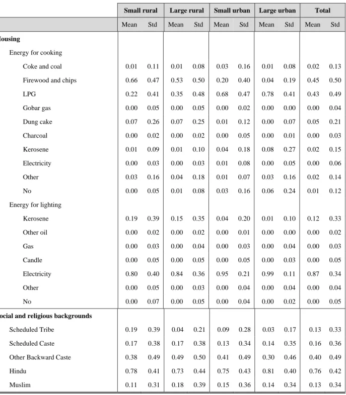
We also generate information on the location characteristics of individual places, using to that effect the Spatial Database for South Asia (Li et al., 2015). This platform combines data from the Census of India, the Household Consumer Expenditure and the Employment and Unemployment modules of the NSS, the Economic Census, administrative records, remote sensing data and crowdsourced data. The Spatial Database for South Asia provides information on a range of socioeconomic indicators, including the urban extent, demographics, jobs, economic activity, infrastructure, ICT, finance, business, living standards, education, health, and environment (Table 1).
Table 1. Summary statistics, by type of location
Small rural Large rural Small urban Large urban Total
Places 579 221 581 25 1406
Observations at household level 45873 10785 33651 5918 96227
Mean Std Mean Std Mean Std Mean Std Mean Std Household expenditure per capita
(current India Rupees per month) 1527 1133 2063 2736 2466 2246 3590 3277 2042 2052
Demographics
Household size 4.94 2.23 4.70 2.16 4.41 2.16 4.15 2.20 4.68 2.21 Children under 6 0.07 0.10 0.07 0.10 0.06 0.10 0.05 0.10 0.06 0.10 Children above 6 0.10 0.11 0.10 0.11 0.09 0.11 0.08 0.11 0.10 0.11 Female adults 0.23 0.13 0.25 0.14 0.24 0.15 0.23 0.16 0.24 0.14 Female dependents 0.03 0.08 0.04 0.09 0.03 0.08 0.03 0.08 0.03 0.08 Male dependents 0.04 0.09 0.04 0.10 0.03 0.09 0.03 0.09 0.04 0.09 Female household head 0.09 0.29 0.13 0.34 0.12 0.33 0.10 0.30 0.11 0.31
Skills
Maximum education of adults (years) 8.40 4.46 9.02 4.41 10.45 4.46 11.06 4.44 9.35 4.57
Assets
Land (0.000 hectares) 0.96 2.14 0.53 1.41 0.19 1.03 0.06 0.64 0.59 1.72
Dwelling
Own 0.95 0.21 0.93 0.26 0.69 0.46 0.58 0.49 0.84 0.37 Rent 0.03 0.17 0.06 0.23 0.27 0.44 0.37 0.48 0.14 0.34 Other 0.02 0.13 0.02 0.13 0.04 0.19 0.05 0.21 0.03 0.16 No 0.00 0.03 0.00 0.02 0.00 0.03 0.00 0.05 0.00 0.03
(Continued)
Table 1. Summary statistics, by type of location (continued)
Small rural Large rural Small urban Large urban Total
Mean Std Mean Std Mean Std Mean Std Mean Std Housing
Energy for cooking
Coke and coal 0.01 0.11 0.01 0.08 0.03 0.16 0.01 0.08 0.02 0.13 Firewood and chips 0.66 0.47 0.53 0.50 0.20 0.40 0.04 0.19 0.45 0.50 LPG 0.22 0.41 0.35 0.48 0.68 0.47 0.78 0.41 0.43 0.49 Gobar gas 0.00 0.05 0.00 0.05 0.00 0.02 0.00 0.00 0.00 0.04 Dung cake 0.07 0.26 0.07 0.25 0.01 0.12 0.00 0.07 0.05 0.21 Charcoal 0.00 0.02 0.00 0.02 0.00 0.05 0.00 0.01 0.00 0.03 Kerosene 0.01 0.09 0.01 0.10 0.04 0.18 0.08 0.27 0.02 0.15 Electricity 0.00 0.03 0.00 0.03 0.01 0.08 0.00 0.05 0.00 0.06 Other 0.03 0.16 0.04 0.18 0.01 0.07 0.03 0.16 0.02 0.14 No 0.00 0.05 0.01 0.08 0.03 0.16 0.06 0.24 0.01 0.12 Energy for lighting
Kerosene 0.19 0.39 0.15 0.35 0.04 0.20 0.01 0.10 0.12 0.33 Other oil 0.00 0.02 0.00 0.02 0.00 0.01 0.00 0.00 0.00 0.02 Gas 0.00 0.03 0.00 0.04 0.00 0.03 0.00 0.04 0.00 0.03 Candle 0.00 0.05 0.00 0.05 0.00 0.05 0.00 0.03 0.00 0.05 Electricity 0.80 0.40 0.84 0.36 0.95 0.21 0.99 0.11 0.87 0.34 Other 0.00 0.05 0.00 0.03 0.00 0.04 0.00 0.04 0.00 0.04 No 0.00 0.07 0.00 0.05 0.00 0.04 0.00 0.02 0.00 0.05
Social and religious backgrounds
Scheduled Tribe 0.19 0.39 0.04 0.21 0.09 0.28 0.03 0.17 0.13 0.33
Scheduled Caste 0.17 0.38 0.17 0.38 0.13 0.34 0.14 0.35 0.16 0.36
Other Backward Caste 0.38 0.49 0.49 0.50 0.41 0.49 0.30 0.46 0.40 0.49
Hindu 0.78 0.41 0.73 0.44 0.75 0.43 0.81 0.40 0.76 0.42
Muslim 0.11 0.31 0.18 0.39 0.15 0.36 0.14 0.34 0.13 0.34
4. Main results
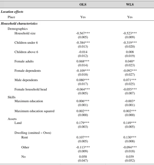
We estimate the benchmark specification using both Ordinary Least Squares (OLS) and Weighted Least Squares (WLS). For the latter, we apply the sample weights at the household level provided by the NSS 2011-12, which ensure that the full data are representative for India. There is considerable debate on whether using OLS or WLS is preferable. No doubt, weighted summary statistics present a representative picture for the underlying population when survey data is used. But when it comes to regression analysis, WLS does not necessarily generate more consistent or more efficient estimators than OLS. Fortunately, the two methods yield very similar coefficients (Table 2).
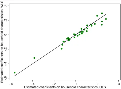
To check whether the difference between the estimators from the two approaches is statistically significant we first apply a test described by Deaton (1997). The test consists of running a weighted regression of the OLS residuals on all the explanatory variables, and evaluating whether the estimated coefficients are jointly equal to zero. The resulting F statistic is 1.36, which is significant at the 0.01 level. However, the R-square of the regression is only 0.041, suggesting a limited difference in explanatory power between the two approaches. We further check the correlation between the parameters estimated with OLS and WLS (Figure 1). For the parameters on household characteristics the correlation coefficient is 0.98; for location effects it is 0.95. Despite these similarities, we conduct the analysis using both OLS and WLS and systematically verify that the conclusions are not dependent on the estimation method. For brevity, in what follows we only present results based on OLS estimators. Results based on WLS estimators are available upon request.
In applying OLS and WLS we implicitly assume that the error terms in the benchmark specification are independently distributed across households and locations. However, the literature on spatial econometrics shows that observations from nearby locations often exhibit similar properties and tend to be spatially correlated. This spatial correlation raises problems similar to those created by the serial autocorrelation of residuals in time-series analysis (Anselin 2003, and Anselin and Rey 2010).
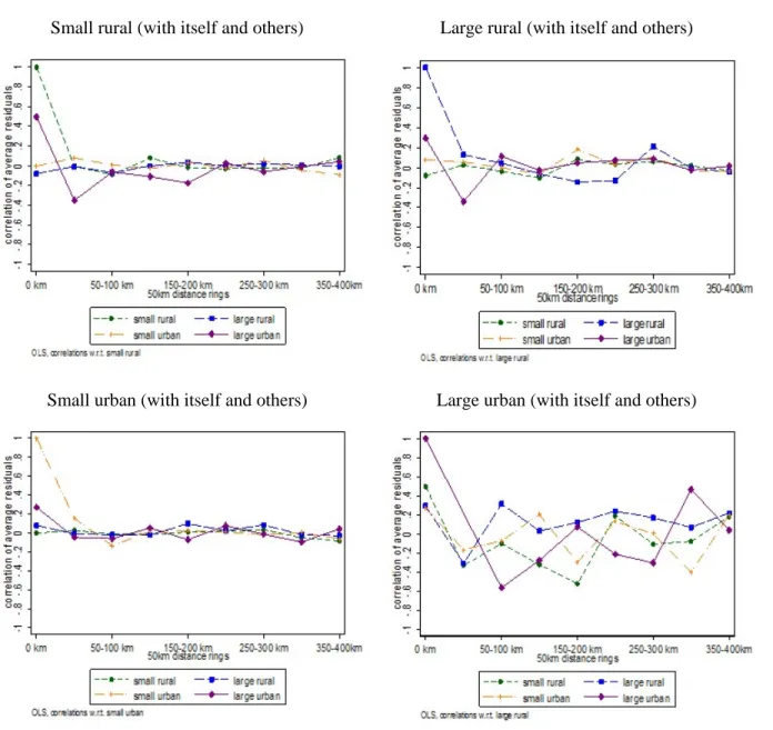
To assess whether there is spatial autocorrelation in our data we run several tests on the residuals of the benchmark specification. First, we average these residuals across the 1,406 places and confirm that the mean residuals by place are distributed closely around zero. This indicates that there is no clustering of residuals at the place level. We then compute the correlation coefficients between mean residuals by place, for all size groups. We do this within each district, and also across districts at distance intervals of 50 kms, up to a maximum distance of 400 km. The resulting correlation coefficients turned out to be small and mostly insignificant (Figure 2). In the case of small rural, large rural and small urban areas, 23 of the 24 correlation coefficients between mean residuals for the same population size groups are statistically insignificant. The only exception is for small urban areas that are distant from each other between 0 and 50 km where the coefficient is around 0.19 and statistically significant. The cross-correlations of group means of residuals that belong to different population size groups shows a similar pattern: 80 of the 81 coefficients are statistically insignificant. In the case of large urban areas, the standard deviations of the correlation coefficients are much larger, because there are much fewer observations. But a vast majority of the correlation coefficients are statistically insignificant.
The lack of spatial autocorrelation of residuals implies that the results of the benchmark regression are not
biased, but it does not imply a lack of spatial correlation in household expenditures per capita. Similar to
the procedure used for the mean residuals by place, we compute the correlation coefficients between
location effects, both within the same district and across districts, at intervals of 50 km. In sharp contrast to
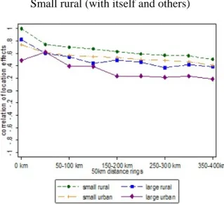
what was observed for the mean residuals, the spatial correlations among location effects are strong and statistically significant (Figure 3). In the case of small rural, large rural and small urban areas, all correlation coefficients are above 0.4 and significantly different from zero for places within the same district. The correlation coefficients gradually decline for districts further apart, but they remain statistically significant for at least 200 km. In the case of large urban areas, the correlation coefficients follow a similar pattern for correlation with places belonging to other population size groups but are more volatile for the correlation coefficient with other large urban areas, because there are few of them.
Table 2 Benchmark regression results
OLS WLS
Location effects
Place Yes Yes
Household characteristics
Demographics
Household size -0.567*** -0.523***
(0.005) (0.009) Children under 6 -0.384*** -0.319***
(0.013) (0.020) Children above 6 -0.014 0.008
(0.012) (0.019) Female adults 0.068*** 0.040*
(0.014) (0.023) Female dependents -0.109*** -0.092***
(0.018) (0.027) Male dependents 0.080*** 0.071***
(0.017) (0.025) Female household head -0.064*** -0.055***
(0.005) (0.007)
Skills
Maximum education 0.006*** -0.003*
(0.001) (0.001) Maximum education squared 0.002*** 0.002***
(0.000) (0.000)
Assets
Land 0.179*** 0.149***
(0.003) (0.005) Dwelling (omitted = Own)
Rent 0.107*** 0.130***
(0.005) (0.008)
Other -0.113*** -0.094***
(0.009) (0.018)
No 0.058 0.039
(0.047) (0.052) Note: Estimated coefficients *significant at 0.1 level, ** significant at 0.05 level, *** significant at 0.01 level.
(Continued)
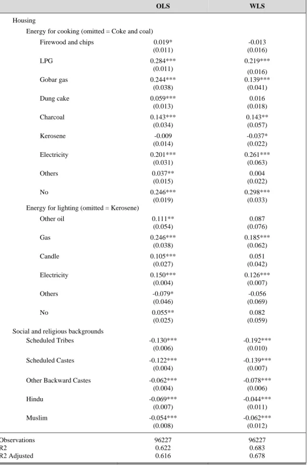
Table 2 Benchmark regression results (Continued)
OLS WLS
Housing
Energy for cooking (omitted = Coke and coal)
Firewood and chips 0.019* -0.013
(0.011) (0.016)
LPG 0.284*** 0.219***
(0.011) (0.016) Gobar gas 0.244*** 0.139***
(0.038) (0.041) Dung cake 0.059*** 0.016
(0.013) (0.018)
Charcoal 0.143*** 0.143**
(0.034) (0.057)
Kerosene -0.009 -0.037*
(0.014) (0.022) Electricity 0.201*** 0.261***
(0.031) (0.063)
Others 0.037** 0.004
(0.015) (0.022)
No 0.246*** 0.298***
(0.019) (0.033)
Energy for lighting (omitted = Kerosene)
Other oil 0.111** 0.087
(0.054) (0.076)
Gas 0.246*** 0.185***
(0.038) (0.062)
Candle 0.105*** 0.051
(0.027) (0.042) Electricity 0.150*** 0.126***
(0.004) (0.007)
Others -0.079* -0.056
(0.046) (0.069)
No 0.055** 0.082
(0.025) (0.059)
Social and religious backgrounds
Scheduled Tribes -0.130*** -0.192***
(0.006) (0.010) Scheduled Castes -0.122*** -0.139***
(0.004) (0.007) Other Backward Castes -0.062*** -0.078***
(0.004) (0.006)
Hindu -0.069*** -0.044***
(0.007) (0.011)
Muslim -0.054*** -0.062***
(0.008) (0.012)
Observations 96227 96227
R2 0.622 0.683
R2 Adjusted 0.616 0.678
Figure 1. Correlation between OLS and WLS estimates
Coefficients on household characteristics
Location effects
Note: The solid line has a 45-degree slope, corresponding to the case where OLS and WLS estimates are identical.
5. Location matters
Combining poverty analysis with urban economics changes the assessment of the relative contribution of household characteristics and location effects to prosperity. Adding more explanatory variables to a
-.6-.4-.20.2.4Estimated coefficients on household characteristics, WLS
-.6 -.4 -.2 0 .2 .4
Estimated coefficients on household characteristics, OLS
77.588.59Estimated location effects, WLS
7 7.5 8 8.5 9
Estimated location effects, OLS
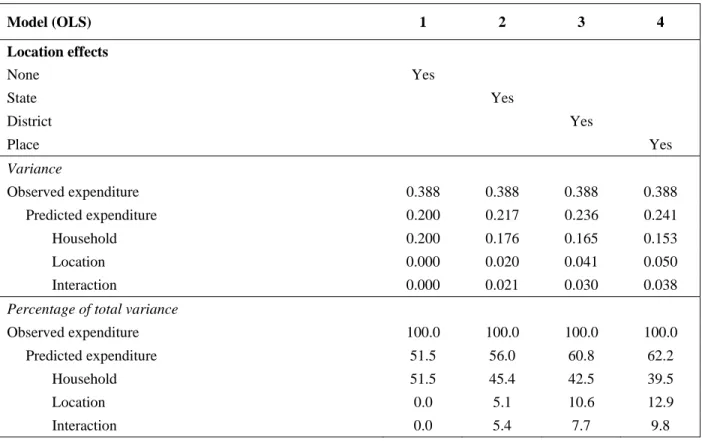
regression always increases the overall explanatory power of the model, but the increase is substantial in this case (Table 3). As a comparator to our benchmark specification, we estimate a model with only household characteristics. The household expenditure predicted by this model explains 51.5 percent of the overall variation in observed household expenditure. By contrast, the predicted expenditure of our benchmark specification with location effects at the place level explains 62.2 percent of the overall variation. For comparison purposes we also conduct two other regressions, with location effects defined at the state and the district levels.
Figure 2. Spatial correlation between average residuals by place
Small rural (with itself and others) Large rural (with itself and others)
Small urban (with itself and others) Large urban (with itself and others)
Figure 3. Spatial correlation between location effects
Small rural (with itself and others) Large rural (with itself and others)
Small urban (with itself and others) Large urban (with itself and others)
Introducing disaggregated location effects not only improves the overall fit of the model: it also corrects
biases in the estimated returns to household characteristics and highlights the correlation between those
characteristics and location effects. An intuitive explanation of this correlation is the sorting of households
through migration decisions. Cities do not attract a random sample of the rural population, but rather
specific population subsets, such as people whose educational attainment is above average. Migration is
not the only mechanism at play. Cities, especially functional ones, also make people with the same
characteristics, such as educational attainment, more productive (Moretti 2004a and 2004b). Conversely,
socially disadvantaged groups tend to concentrate in some of the least productive places. For example,
households belonging to Scheduled Tribes often live in forest areas in India. Not taking this sorting
explicitly into account results in overstating the negative impact of their social background on their household expenditure per capita.
Table 3. Variance decomposition
Model (OLS) 1 2 3 4
Location effects
None Yes
State Yes
District Yes
Place Yes
Variance
Observed expenditure 0.388 0.388 0.388 0.388
Predicted expenditure 0.200 0.217 0.236 0.241
Household 0.200 0.176 0.165 0.153
Location 0.000 0.020 0.041 0.050
Interaction 0.000 0.021 0.030 0.038
Percentage of total variance
Observed expenditure 100.0 100.0 100.0 100.0
Predicted expenditure 51.5 56.0 60.8 62.2
Household 51.5 45.4 42.5 39.5
Location 0.0 5.1 10.6 12.9
Interaction 0.0 5.4 7.7 9.8
Note: From our benchmark specification it follows that:
∙
∙ 2 ∗ ∙ ,
This point can be illustrated in a more formal way by decomposing the variance of observed household expenditure per capita. There are several ways to do this (see, for instance, Combes, Duranton, and Gobillon 2008). A relatively straightforward approach is to algebraically decompose the total variance into four components: 1) the variance of the returns on household characteristics, 2) the variance of location effects, 3) twice the covariance between returns to household characteristics and location effects, and 4) the variance of the residuals.
The contribution of these four components to the overall variation in household expenditure per capita
changes quite substantially as locations are introduced in the regression and disaggregated with increasing
granularity (Table 3). The contribution of household characteristics falls from 51.5 percent of the total
variance in a model without location effects to 39.5 percent in our benchmark specification. In parallel, the
explanatory power of location effects increases from 0 to 12.9 percent, whereas the contribution of the interaction term increases from 0 to 9.8 percent.
As a robustness check, we also decompose the explained variance under the various specifications following a framework based on the Shapley-value function (Huettner and Sunder 2012, and Shorrocks 2013). This methodology allocates the explained variance to the individual explanatory variables based on their marginal contributions. The results, available on request, confirm the growing importance of location as the spatial granularity of the analysis increases.
Locations effects not only attenuate the contribution of household characteristics: they also lead to statistically different estimates of their effects. To illustrate this point we classify household characteristics into four groups: demographics, skills, assets and housing, and social and religious background. For each group of characteristics, we compare the coefficients estimated with our benchmark specification to the coefficients estimated in the model without location effects. Chi-square tests confirm that the estimates are significantly different for all four groups of characteristics. The difference remains statistically significant when comparing with the other two models, in which location effects are defined at state and district levels.
This results suggest that conducting poverty or spatial analyses at the state or district levels yields biased results, and that further spatial disaggregation is required to analyze the rural-urban transformation.
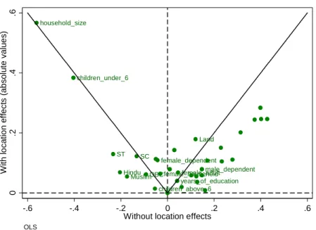
Introducing location effects at a disaggregated level also changes the interpretation of the contribution some household characteristics make to household expenditures per capita. We plot the absolute values of the estimated coefficients on household characteristics from our benchmark specification against the estimates from the model without location effects. For educational attainment, we report the marginal effect at the average years of schooling instead of the estimated coefficients. We do so because the square of education variable is also entered in the benchmark specification, to account for possible non-linearity in returns to skills. The estimated coefficients (and marginal effect) decline for 24 of the 35 household characteristics considered, and remain unchanged for only three of them (Figure 4).
One of the most dramatic changes concerns the estimated effects of the household’s social and religious background. Belonging to a Scheduled Tribe, a Scheduled Caste or Other Backward Castes has traditionally been associated with enjoying lower household expenditure per capita. Hindu, and especially Muslim households are also seen as faring worse than Christian households. However, when using our benchmark specification these “stigma” effects decline substantially, as shown in Figure 5. The estimated coefficient on being Hindu falls (in absolute terms) from -0.204 to -0.069, and the coefficient on being Muslim falls (in absolute terms) from -0.173 to -0.054. The drop is similar for the coefficient associated with belonging to Scheduled Tribes, which falls (in absolute terms) from -0.233 to -0.130. The estimated coefficients remain all statistically significant, but it is legitimate to wonder whether ever greater spatial granularity in the analyses would not make them fade away altogether.
6. Cities and catchment areas
The estimated location effects provide a useful metric to evaluate the performance of difference places
across India. To make this metric more intuitive, we rescale the location effects by subtracting the median
across all 1,406 places. The distributions of location effects are quite spread out. The value of the rescaled
Because household expenditures per capita are measured in log, these figures should not be interpreted as percentages. But they can be converted easily, and they imply that households with the same characteristics have expenditures per capita which are on average 131 percent above the median in the top locations, and 50 percent below the median in bottom locations.
Figure 4. Coefficients on household characteristics
Note: Coefficients on the left of the vertical dotted line are negative, while those on the right are positive. The solid line has a 45-degree slope, corresponding to the case where coefficients are identical.
Figure 5. Coefficients on social and religious backgrounds
household_size
children_under_6
ST Hindu
Muslim SC
OBC
children_above_6 female_dependent
female_household years_of_education
female_adult Land
male_dependent
0.2.4.6With location effects (absolute values)
-.6 -.4 -.2 0 .2 .4 .6
Without location effects
OLS
w/o Location w/ Location
w/o Location w/ Location
w/o Location w/ Location
w/o Location w/ Location
w/o Location w/ Location
-.25-.2-.15-.1-.050Estimated coefficients
Hindu Muslim OBC SC ST
OLS
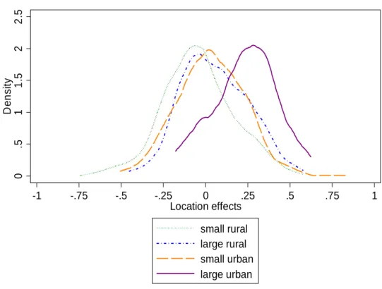
Unsurprisingly, location effects are generally higher in urban areas than in rural areas and in places with a larger population than otherwise, as shown in Figure 6. T-tests show that the mean of location effects for small rural areas is smaller than that for large rural areas, and the mean of location effects for small urban areas is smaller than that for large urban areas. Kolmogorov-Smirnov tests further confirm that the distribution of the location effects for the two rural groups differ significantly, as also do the distributions of location effects for the two urban groups.
Figure 6 Distribution of location effects, by population size groups
Note: Location effects are measured relative to the median place in India, and expressed in log. The percent equivalent of a location effect ∗ expressed in log relative to the median place is 100 ∙ ∗ 1
However, the ranking of places is not as straightforward as the notion of a rural-urban divide would suggest.
The four distributions have a wide common support, with location effects being sizeable in some rural areas, and clearly below the median in some urban areas. The notion of a rural-urban divide is further undermined by the fact that the distributions of location effects for large rural areas and for small urban areas are difficult to distinguish from each other. T-test cannot reject that the means of the location effects for the two groups are the same. Kolmogorov-Smirnov test cannot reject that the distributions of the location effects for the two groups are the same either. Thus, consistent with the findings by Chatterjee et al. (2015), India seems to be characterized by a rural-urban gradation more than by a rural-urban divide.
Location effects depend not only on the places themselves: they are also influenced by their neighborhoods.
0 .5 1 1. 5 2 2. 5 De n s it y
-1 -.75 -.5 -.25 0 .25 .5 .75 1
Location effects small rural large rural small urban large urban
nominal consumption based, OLS
to different population size groups. This suggests that distance, and especially “distance to what?” matters.
Because of this high spatial correlation, places near solid performers can be expected to perform well. This is in line with the idea of clustering, and of productive spillovers from the core of the cluster to its periphery.
It is also consistent with evidence from advanced economies where the effect of agglomeration economies attenuates with distance (Rosenthal and Strange 2004 and 2008, and Melo et al. 2009). Bottom locations tend to cluster as well, suggesting that improving their performance might be difficult, because that requires countering bad-neighborhood effects.
The importance of “distance to what?” can be illustrated by comparing the places surrounding Delhi and Faridabad to those surrounding Bangalore (Figure 7). Both urban agglomerations are among India’s best performers, although Bangalore (with a location effect of 0.512) arguably does better than Delhi and Faridabad (0.415 on average). However, the places surrounding Delhi and Faridabad register much higher location effects on average than those surrounding Bangalore. In fact, location effects for small urban and large rural places within 50 km of Delhi are on average stronger than the average location effect of Delhi and Faridabad. The spread of places with sizeable location effects is also much broader around Delhi and Faridabad than around Bangalore, exceeding 0.1 (a 10.5 percent premium) up to 200 km away from the core. In contrast, the location effects of small rural and large rural places surrounding Bangalore fall below 0.1 after 100 km. This comparison suggests that Bangalore is more productive than Delhi and Faridabad, but its periphery is less productive than the periphery of Delhi and Faridabad.
Figure 7. Delhi-Faridabad versus Bangalore
Delhi-Faridabad Bangalore
Note: Location effects are measured relative to the median place in India, and expressed in log. The dotted purple line represents the (average) location effects of the central cities. The other lines represent the average location effects of places surrounding the cities by 50km rings of distance.
Building on the insights from this comparison, we classify all 1,406 places into four tiers. We do so based on both their location effects and their neighborhoods, but ignoring their administrative classification as
-.2-.10.1.2.3.4.5.6Location effects
0 km 0-50 km 50-100 km 100-150 km 150-200 km
Distance to a mega city (km) small rural large rural small urban
nominal consumption based, OLS
-.2-.10.1.2.3.4.5.6Location effects
0 km 0-50 km 50-100 km 100-150 km 150-200 km
Distance to a mega city (km) small rural large rural small urban
nominal consumption based, OLS