Applications of high-resolution imaging for planetary systems

(1)

Applications of high-resolution imaging for planetary systems

A thesis submitted to attain the degree of DOCTOR OF SCIENCES of ETH ZURICH

(Dr. sc. ETH Zurich)

presented by Silvan Hunziker

Master of Science ETH in Physics ETH Zürich

born on July 12, 1987

citizen of Gontenschwil (AG), Switzerland

accepted on the recommendation of Prof. Dr. H. M. Schmid

Prof. Dr. S. P. Quanz Prof. Dr. A. Refregier

2020

(2)

(3)

— Douglas Adams,The Hitchhiker’s Guide to the Galaxy

(4)

(5)

Abstract

The first detection of an exoplanet around a solar-type star in 1995 has marked the beginning of a new field in astronomy that has since evolved into one of the most important and popular research fields. In only a few years, multiple techniques to detect and characterize planets around stars outside the Solar System have been identified and developed. One such technique is referred to as direct imaging, and it simply describes the technique of taking an image from a planet and being able to visibly separate it from its host star. Direct imaging requires very large telescopes like the VLT in Paranal/Chile with specialized instrumentation in order to achieve the high resolution and sensitivity, which is necessary to identify the faint signal of an exoplanet next to its much brighter host star. This thesis is divided into three parts, each of which discusses a project that concerns itself with a particular aspect of high contrast imaging of exoplanets or circumstellar disks with large ground based telescopes.

THE FIRST PARTis dedicated to modeling and subtracting the thermal infrared background in direct imaging observations of exoplanets. Imaging at longer wavelengths, upwards of 3µm, suffers from strong infrared (IR) background, which is caused by thermal photons from various sources. Instruments for imaging at these separations have to be cooled down to very low temperatures to not be overwhelmed by the background radiation, but components outside of the instrument, like the large main mirror of the telescope, cannot be cooled down. In addition, ground based observations suffer from the thermal background that is caused by the Earth’s warm atmosphere. The thermal background quickly starts being the limiting factor at long wavelengths and special techniques are required to limit its impact on the observations.

The usual procedures involve the observation of the empty sky close to the target, which in- creases the observation time without any direct contribution to the observation, but it allows to calibrate the IR background. Since the background can change significantly on short and long timescales, the IR background observations have to be repeated frequently to allow for the best possible calibration. Insufficient background sampling can have a significant negative impact on the quality of the reduced data. This work presents a new algorithm that can be applied to improve the subtraction of the IR background in existing and new direct imaging data. The algorithm is based on principle component analysis (PCA), which is applied to the background calibration images to produce a model of the IR background and subtract it from the data. Application of the algorithm to many different datasets has shown promising results, even when the background was sampled infrequently, and the algorithm was implemented as i

(6)

The work presented inTHE SECOND PARTis dedicated to the results of a direct imaging survey for reflected light from exoplanets around nearby bright stars. Reflected light refers to the light that was emitted by the host star and reflected on the planetary surface, contrary to the thermal radiation, which is emitted by the planet itself. The search aimed at the detection of mature planets that have evolved beyond their formation stage and have cooled down towards their respective equilibrium temperatures, just as observed for all Solar System planets. The thermal emission of such cold planets peaks at IR wavelengths>5µm and is therefore difficult to directly image, however, shorter wavelength observations are used to search for their reflected light signatures. The direct detection of an evolved exoplanet has not been achieved yet due to the expected large brightness contrast between the planet and its host star, but imaging of reflected light with modern instruments could make this possible. The survey described in this work made use of the Zurich Imaging Polarimeter (ZIMPOL) at the Very Large Telescope (VLT), which operates at 600-900 nm. ZIMPOL can distinguish between the polarized reflected light from a planet’s atmosphere and the largely unpolarized direct starlight of its host star.

The survey has not yet resulted in the detection of an exoplanet, but it concludes that the high sensitivity of ZIMPOL would enable the detection of a Jupiter sized planet around either star in Alpha Centauri in one observing night. This unprecedented performance has also lead to improved contrast limits for reflected light at visible wavelengths around all other stars in the survey.

THE THIRD PARTis a comprehensive study of the reflected light from the protoplanetary disk around the young stellar binary HD142527. Protoplanetary disks consist of gas and dust which are remnants of the star formation and slowly disappear during the first few million years of its lifetime. During this time, the dust size evolves and smaller grains coagulate into larger grains and eventually form comets, asteroids and planets. The careful study of such disks helps us to better understand the processes that lead to the formation of planets. Recent development of powerful adaptive optics (AO) systems for direct imaging with high sensitivity and resolution have revealed a number of such disks around young stars in nearby star forming regions. The detection of scattered light from protoplanetary disks is one problem, but the measurement of the scattered flux is even more challenging, because it involves a careful calibration of the instruments and consideration of a number of instrumental and physical effects that alter the observed signal. The study in this work shows how the reflected light and its degree of polarization can be measured with high precision and how certain instrumental and physical effects can change the measured result. It also shows how the reflected light measurements can be used to infer some of the optical properties of the dust in the observed disk and how the properties are correlated with each other. By comparing the measurements to simulations of light scattering processes it was possible to constrain some of the optical properties and relate them to physical dust properties. The physical properties show for example signs of dust growth due to the presence of large dust grains (>2.5µm) on the disk surface, which are absent in interstellar dust clouds. The study also discusses problems inherent to the observations ii

(7)

iii

(8)

(9)

Zusammenfassung

Die erste Detektion eines Exoplaneten um einen sonnenähnelichen Stern im Jahr 1995 hat den Beginn eines neuen Forschungsbereichs in der Astronomie markiert und sich seither weiterentwickelt zu einem der wichtigsten und populärsten Bereiche der Astronomie. In nur wenigen Jahren wurden mehrere Techniken zur Detektion und Beschreibung von Planeten ausserhalb des Sonnensystems erkannt und weiterentwickelt. Eine solche Technik ist die direkte Abbildung eines Planeten, also die visuelle Separation des Planeten von seinem Stern auf einem Bild. Für die direkte Abbildung eines Exoplaneten sind sehr grosse Teleskope wie das Very Large Telescope (VLT) in Paranal/Chile und spezialisiert Instrumente nötig, welche die hohe Auflösung und Sensitivität erreichen können, die nötig ist, um das schwache Signal eines Exoplaneten in der Nähe seines viel helleren Sterns identifizieren zu können. Diese Dissertation spaltet sich in drei Teile, welche sich alle mit einem speziellen Aspekt der Abbil- dung von Exoplaneten und zirkumstellaren Scheiben mit grossen erdgebundenen Teleskopen befassen.

DER ERSTETEILbefasst sich mit dem Modellieren und Entfernen der thermischen infraroten

(IR) Hintergrundstrahlung bei direkten Beobachtungen von Exoplaneten. Beobachtungen bei langen Wellenlängen von mehr als 3µm sind stark beeinträchtigt von Hintergrundstrahlung thermischer Photonen aus unterschiedlichen Quellen. Instrumente, welche im IR Bereich operieren müssen deshalb stark gekühlt werden, um die Hintergrundstrahlung zu minimieren. Komponenten wie der grosse Hauptspiegel des Teleskops, welche sich ausserhalb der Instrumente befinden, können allerdings nicht gekühlt werden. Eine zusätzliche Hintergrund- strahlung für Beobachtungen von der Erdoberfläche wird von der warmen Erdatomsphäre produziert. Die kombinierte thermische Hintergrundstrahlung ist oft der limitierende Faktor für Beobachtungen bei IR Wellenlängen und spezielle Techniken werden benötigt, um dessen Einfluss auf die Beobachtungen zu minimieren. Eine der Techniken beinhaltet die Beobach- tung des Himmels in der Nähe des Ziels, was die Beobachtungszeit vergrössert ohne zu der eigentlichen Beobachtung der Ziels beizutragen, es aber ermöglicht den IR Hintergrund zu kalibrieren. Da sich der IR Hintergrund auf kurzen und langen Zeitskalen verändern kann, müssen die Beobachtungen des Himmels regelmässig wiederholt werden, um eine gute Kali- brierung zu ermöglichen. Eine ungenügende Kalibrierung kann einen negativen Einfluss auf das Resultat der Beobachtungen haben. Diese Arbeit präsentiert einen neuen Algorithmus, der zur Modellierung und Entfernung des IR Hintergrunds in existierenden und zukünftigen v

(10)

Algorithmus wurde mit vielversprechenden Resultaten auf mehrere Datensätze angewandt, sogar wenn die Kalibrierungsbeobachtungen nicht regelmässig durchgeführt wurden, und wurde als zusätzliches Modul in den PynPoint Datenreduktionsalgorithmus implementiert.

Die Arbeit imZWEITENTEILbeschäftigt sich mit den Resultaten einer Studie zur Suche nach reflektiertem Licht von Exoplaneten um nahe, helle Sterne. Reflektiertes Licht bezieht sich auf jenes Licht, welches von einem Stern erzeugt und von einem Planeten in der Nähe des Sterns reflektiert wird, im Gegensatz zur thermischen Strahlung, welche vom Planeten selber erzeugt wird. Die Suche richtet sich nach älteren Planeten, lange nach ihrer Entstehungsphase, welche abgekühlt sind in die Nähe ihrer Gleichgewichtstemperatur, wie es zum Beispiel für alle Planeten im Sonnensystem der Fall ist. Die thermische Strahlung solcher kalter Planeten ist maximiert in IR Wellenlängen von>5µm und deswegen schwierig zu beobachten von der Erde. Beobachtungen bei kürzeren Wellenlängen können jedoch trotzdem Signale von reflektiertem Licht entdecken. Die direkte Abbildung eines entwickelten Planeten war bisher unmöglich durch den sehr hohen Helligkeitskontrast zwischen dem reflektierten Licht eines Planeten und dem direkten Licht seines Sterns, neu entwickelte hoch sensitive Instrumente könnten dies allerdings ermöglichen. Die hier beschriebene Studie nutzt das Zurich Ima- ging Polarimeter (ZIMPOL) am Very Large Telescope (VLT), welches in Wellenlängen von 600-900 nm operiert. ZIMPOL kann zwischen dem polarisierten Anteil des reflektierten Lichts eines Planeten und dem hauptsächlich unpolarisierten direkten Licht des Sterns unterschei- den. Die Suche nach einem Planeten in reflektiertem Licht mit ZIMPOL war bisher nicht erfolgreich, aber die vorläufigen Resultate zeigen, dass die hohe Sensitivität von ZIMPOL die Detektion eines Exoplaneten der Grösse von Jupiter um einen der Sterne in Alpha Centauri in einer einzigen Beobachtungsnacht möglich machen könnte. Diese beispiellose Leistung resultierte zusätzlich in verbesserten Limiten für die Detektion von reflektiertem Licht bei sichtbaren Wellenlängen für alle anderen beobachteten Sterne.

DER DRITTE TEIList eine umfassende Studie des reflektierten Lichts der protoplanetaren

Scheibe um den Doppelstern HD142527. Protoplanetare Scheiben bestehen aus Gas und Staub, den Überbleibseln aus der Entstehung des Sterns, welche in den ersten Millionen Jahren nach der Sternentstehung langsam aus dem System verschwinden. Die kleinen Staub- teilchen entwickeln sich in dieser Zeit zu grösseren Teilchen und schlussendlich zu Kometen, Asteroiden und Planeten. Das sorgfältige Studium solcher Scheiben ermöglicht Einblicke in die Prozesse dieser Entwicklung und verbessert unsere Verständnis der Planetenentstehung.

Die Entwicklung von leistungsfähigen adaptiven Optiken (AO) für grosse Teleskope ermöglicht Beobachtungen mit grossen Sensitivität und Auflösung, und hat über die letzten Jahre eine Fülle solcher Scheiben um junge Sterne in nahen Sternentstehungssystemen offenbart. Die Detektion solcher lichtschwachen Scheiben ist nicht einfach, aber die Messungen des reflektierten Lichts ist noch anspruchsvoller, da es eine sorgfältige Kalibrierung des Instruments vi

(11)

verfälschen können. Die hier präsentierte Studie zeigt, wie das reflektierte Licht und die Polarisation der grossen und hellen Scheibe um HD142527 mit hoher Präzision gemessen werden können, und wie die Messungen von instrumentellen und physikalischen Effekten beeinflusst werden. Die Studie zeigt ebenfalls, wie die Messungen einsetzt werden können, um die optischen Eigenschaften des Staubes zu einzuschränken und wie die einzelnen optischen Parameter miteinander korreliert sind. Dies war möglich durch den Vergleich der Messungen mit Simulationen von Lichtstreuung an optisch dicken Staubverteilungen und hat es ebenfalls ermöglicht die physikalischen Eigenschaften des Staubes in HD142527 einzuschränken. Die physikalischen Eigenschaften zeigen die Anwesenheit von grossen Staubteilchen (>2.5µm), welches als typischen Anzeichen für das Wachstum der Staubteilchen interpretiert wird, da solche grosse Staubteilchen normalerweise im interstellaren Staub nicht beobachtet werden. Die Studie diskutiert ebenfalls einige Probleme mit den Beobachtungen, die während der Analyse erkannt wurden und diskutiert Verbesserungsvorschläge für zukünftige Beobachtungen.

vii

(12)

(13)

1 Introduction

1.1 Direct imaging of extra-solar planetary systems

In the field of exoplanetary research, direct imaging refers to the classical way of directly detecting light from a source close to its host star (see Seager, 2010). This could be either an exoplanet or a circumstellar disk. Indirect methods, on the other hand, use the light of the star itself to infer the presence of objects in its vicinity (see Seager, 2010). Examples are the transit or radial velocity methods that were the first and are still the most successful methods for finding and characterizing exoplanets. In addition, the analysis of the stellar spectral energy distribution (SED) has proven to be very successful in detecting and characterizing circumstellar disks (Malfait et al., 1998). A direct detection would be preferable to any other methods because it provides the most complete set of information about the object. The information from direct imaging can be used to determine the orbital parameters as well as the emitted and reflected light spectrum of the exoplanet’s surface and atmosphere (e.g. Sudarsky et al., 2000). This can provide all the necessary information about the planetary orbit, size, mass and even the composition of its atmosphere. Similar measurements on circumstellar disks provide information about the composition and morphology of protoplanetary and debris disks (e.g. Quanz et al., 2011; Milli et al., 2019). Such disks are usually found around young stars and are places where planet formation is ongoing or has already happened in the past (Keppler et al., 2018).

Despite the great advantages of direct imaging, only few circumstellar disks and even fewer exoplanets have been directly observed to date because of a few great technical challenges.

One major problem is caused by the high resolution, which is necessary to be able to detect such faint objects located in close proximity to their bright host star. The theoretical resolution limit for a telescope with aperture sizeDobserving at a wavelengthλcan be calculated with the diffraction limit of the aperture 1.22λ/D. This corresponds to an angular resolution of around 30 mas for an observation at a typical wavelength of 1µm with an aperture size that corresponds roughly to the size of the Very Large Telescope (VLT). For a star at distance of 1

(18)

30 pc, this angular resolution translates into a spacial resolution of only∼1 astronomical units (AU). This shows, just from the resolution limit alone, how even today’s larges telescopes would struggle to directly image an Earth-like planet around a star at distances of only 30 pc. In reality, optical aberrations and other technical challenges often lead to an additional degradation of the resolution to values around 2−5λ/D(Schmid et al., 2018).

For ground based observatories, even this kind of resolution cannot be achieved without considerable technical efforts, because of atmospheric disturbances. Light from a distant source has to travel through the Earth’s atmosphere before arriving at the telescope. Density gradients and fluctuations in the atmosphere disturb the wavefront of the passing light and create what is commonly referred to as "seeing". The atmospheric seeing deteriorates the minimum resolution of any telescope to a value determined solely by the turbulence in the atmosphere, which is usually a resolution of order 1". This problem was solved with the development of adaptive optics (AO) systems. AO systems on large telescopes use wavefront sensors (WFS) and a deformable mirror (DM) to measure the aberrations of the wavefront that arrives at the telescope and correct the wavefront in real-time (Davies and Kasper, 2012).

This allows large ground based telescopes to operate much closer to the theoretical resolution limit, which is needed for the detection of exoplanets and circumstellar disks.

However, for the detection the faintest objects, it has been necessary to develop additional ways to distinguish between the stellar light and the light emitted or reflected by a planet or a circumstellar disk close to the star. Even with a perfect AO system, the resolution cannot exceed the theoretical limitations, which can still completely drown out objects with a large brightness contrast to the star. Coronagraphs have been used for a long time to mitigate this problem by physically blocking some of the stellar light, however, a range of differential imaging techniques have been developed in recent years to uncover even fainter objects. Differential imaging techniques exploit the different properties of the light emitted by the observed star and light from a source close to the star to improve the sensitivity of the observations. According to the property of the light that is exploited, these techniques are called angular differential imaging (ADI), spectral differential imaging (SDI) and polarimetric differential imaging (PDI). The principle of each method will be quickly discussed in Section 1.2.

1.1.1 Adaptive optics

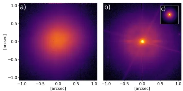
Fig. 1.1(a) and (b) show two images taken with the ZIMPOL/SPHERE instrument at the Very Large Telescope in visible wavelengths. The figure showcases the power of the extreme AO system SAXO (Petit et al., 2008) in SPHERE by comparing two images that were taken with and without active AO correction. The resolution of the seeing affected point spread function (PSF) is around∼0.5", with activated AO system the resolution improves significantly to∼0.03".

The DM in SAXO is equipped with 41×41 actuators that correct the shape of the mirror with a frequency of around 1 kHz (Fusco et al., 2006). This is fast enough to deliver an excellent correction of the wavefront if the timescale of the turbulence in the atmosphereτ0is roughly

2

(19)

Figure 1.1: Images of the star HD142527 with the VBB filter (∼735nm) of ZIMPOL/SPHERE at the VLT with logarithmic color scale. (a) was taken without AO correction due to a temporary failure of the AO system during the observation. (b) was taken with active and perfectly working AO system during the same observing run. (c) shows a simulation of the best possible resolution for a VLT sized circular aperture and with the VBB filter. The images of the star were taken during excellent observing conditions with an atmospheric seeing around 0.5", which is reflected in the size of the star without AO system. All frames have the same angular scale.

2 ms or above, which is usually the case at the site of the VLT. The AO correction is also limited spatially. Because of the finite amount of actuators of the DM, only the part of the light which is not too far from the center of the PSF can be focused into the peak of the PSF. In the case of SAXO, this distance is about 20λ/D¹. The effect of this can be seen in Fig. 1.1(b), where the AO correction produces a ring (AO control ring) with increased brightness at around 20λ/D separation from the central peak of the PSF and a dark hole at smaller angular separations.

The light at separations smaller than 20λ/Dcan be focused into the peak by the AO system, while the light outside is almost completely unaffected. As a result of that, the performance of an AO system can never perfectly reconstruct the best possible PSF shown in Fig. 1.1(c), which shows the Airy pattern of a VLT sized aperture convolved with the VBB filter curve. The performance of the AO system is often quantified with the Strehl ratio, which is defined as the ratio between the peak intensity of the PSF and the maximum possible peak intensity for the optical system. High Strehl ratios∼0.9 can be achieved in the near-IR but are difficult to achieve in the visible wavelengths (Schmid et al., 2018). Since light can only be focused up to an angular separation of 20λ/D, shorter wavelengths have a natural disadvantage with regard to the Strehl ratio.

1The angular separation is equal to^N_2D^λfor an AO system withN×Nactuators (see Traub et al., 2010).

3

(20)

Figure 1.2: The radial intensity profile of the VBB filter PSF shown in Fig. 1.1(a), compared to the total noise and the different noise contributions on the right. The total noise was measured as the standard deviation of the PSF intensity at different separations. The photon noise was calculated as the square-root of the intensity profile divided by the square-root of the detector gain. The read noise of the detector can be found in the SPHERE/VLT user manual. The residual noise was calculated by subtracting photon and read noise from the total noise and consist mainly of speckle noise.

1.1.2 Point spread function

The PSF is the image of a point source (usually a star) produced by the optical system of the telescope and its instruments. The perfect PSF of a telescope with a circular aperture would roughly look like the Airy pattern shown in Fig. 1.1(c), but a real system is affected by aberrations that additionally spread a fraction of the light (see Fig. 1.1(b)) across the field- of-view (FOV). The additional features of the PSF are major sources of noise and contribute to hiding faint signals in the vicinity of a star. In addition, the shape of the PSF can also be variable over very short timescales (∼1 ms), depending on the observing conditions and AO performance. The AO control ring at 20λ/Dcan be a significant limiting factor for observations as well, especially for observations of extended objects like circumstellar disks (see Chapter 4).

These problems are usually more significant at shorter wavelengths in the visible and near-IR, because the disturbing features are more pronounced at shorter wavelengths and the AO control ring is located at separations around∼1", where many of the interesting sources are located around stars in the closest star-forming regions.

1.1.3 Noise properties

Successful direct imaging observations and measurements require a good understanding of the main noise contributions and how the different contributions can be mitigated with specialized observing strategies and data reduction algorithms. Fig. 1.2 shows a summary of the dominant noise components, which were determined for the single VBB filter image shown in Fig. 1.1(b). The noise is calculated only as a function of the distance to the star, 4

(21)

because in most cases the PSF is close enough to being azimuthally symmetric for this sort of representation to be valid.

One of the main contributions is the photon noise from the stellar PSF, which is proportional to the square-root of the PSF intensity. In the best case scenario, the photon noise would dominate the noise at all separations because it is the fundamental statistical noise source that arises when photons are counted. In the photon noise dominated case, the signal to noise ratio (S/N) of an observed signal can only be increased by collecting more photons, i.e.

observing for a longer amount of time.

Far away from the center of the PSF, where photon counts are low, the dominating noise source is either detector read noise or, at least for longer wavelengths, the infrared background noise.

Read noise is generated by the detector electronics when the detector pixels values are read.

This is basically just an additional uncertainty, which is added to all pixel values and is roughly equal for each pixel even when no photons were registered. The infrared background noise is produced by thermal photons emitted by the sky, the telescope or the instrument itself, and is therefore mostly a problem for observations at longer near- and mid-IR wavelengths. The background is roughly constant across the FOV as well but it can be time dependent. The thermal background can partially be mitigated by cooling down the instrument to very low temperatures. In the example of the visible light observation shown Fig. 1.2, the constant noise contribution is completely dominated by read noise at all separations>0.5".

The last important source of noise is usually called speckle noise and it dominates at separations closer to the center of the PSF. Speckles are caused by wavefront errors from the imperfect optics and correction of the AO system, which appear in the image as faint copies of the stellar PSF (Traub et al., 2010). Their intensity can vary on very short timescales (transient speckles), usually of order∼1ms, or they can stay in the same place for a long time (pinned speckles). For the example presented in Fig. 1.2, speckle noise is the dominating source of noise at separations<0.5". The speckle noise quickly decreases with increasing separation from the star, however, since most of the interesting objects in exoplanetary science are very close the star, it remains a major problem in direct imaging. The differential imaging strategies which will be discussed quickly in Section 1.2 were developed with the purpose of reducing speckle noise in direct imaging observations.

1.2 Differential imaging techniques

The limit of how faint a source can be with respect to the star and still be detectable is commonly referred to as the contrast limit. Since most of the noise in the vicinity of the star is caused by light of the star itself, subtracting the light of the star results in an image with significantly less noise and improved contrast limits. Differential techniques are designed to achieve this goal by taking advantage of knowledge about the differences of the light from the on-axis source (star) and any faint off-axis objects. The different techniques are grouped and named according to the property of the data that is exploited to achieve this goal. All 5

(22)

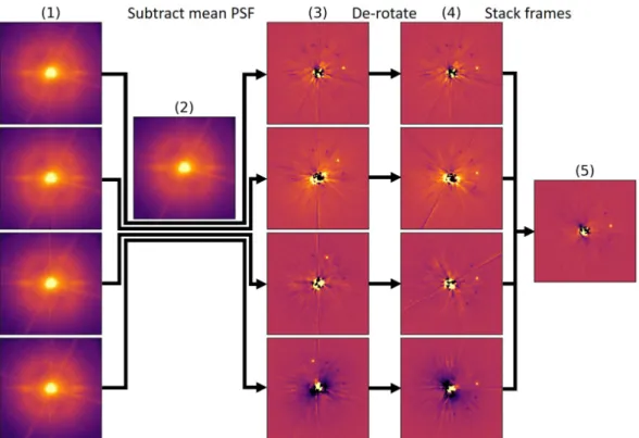
Figure 1.3: Illustration of the angular differential imaging method with real data from SPHERE/ZIMPOL in the VBB filter but with an artificially added point source with a brightness 5·10⁻⁴times weaker than the star, seen at four different field rotations. The five columns illustrate the main steps of this method. (1) The star is observed at different field rotations.

(2) The average over all frames with different rotations is used to produce a general model of the stellar PSF. (3) The model is subtracted from each observation in (1) separately. (4) The observations are de-rotate to a common parallactic angle. (5) The de-rotated frames are stacked to reduce noise while conserving the signal of the point source.

techniques rely on specialized observation techniques and use specialized data reduction algorithms. However, for achieving the best results, specialized instruments are needed as well to perform the observations in the most optimal way and limit the number of systematic noise sources. Additional information about differential techniques for direct imaging can be found in various reviews like Seager (2010).

1.2.1 Angular differential imaging

Instruments at ground based telescopes like the VLT are often equipped with a de-rotator that optically rotates the image from the telescope into the equatorial coordinate system before it arrives at the detector. This allows to perform long exposures without circumstellar signals being smeared out by the apparent rotation of the sky and consecutive images can be combined without first having to de-rotate them into the same coordinate system. However, ADI relies on the rotation of the Earth to help produce a model of the stellar PSF and some 6

(23)

of the static aberrations from the instrument. This model is then subtracted from the data to remove the PSF along with the static noise features, which improves the contrast limits of the data significantly (Marois et al., 2008). The situation is illustrated in Fig. 1.3 for an artificial point source that simulates the signal of a planet close to the host star. In the four consecutive images, the planet signal seemingly rotates by 20^◦in each frame due to the rotation of the sky during the night. The PSF of the star and most of the static aberrations, however, stay roughly the same if the AO performance and observing conditions do not change significantly in between consecutive exposures. As a result of that, the average PSF can be used as a model for the PSF and the static aberrations. The model can then be subtracted from the initial observations, which removes a large fraction of the noise from each image individually. The individual images are then de-rotated into a common equatorial coordinate system to compensate for the sky rotation and combined to further reduce the noise while simultaneously conserving the signal of the point source.

One of the main problems of this method is the self-subtraction of the circumstellar signal, especially for extended sources like face-on circumstellar disks (Milli et al., 2012). Since the observations, that are used to model the noise, contain the signal as well, the model of the noise which is subtracted from the data always contains a fraction of the signal. This results in a partial subtraction of the signal. This effect interferes with the detection of point sources as well as extended sources like circumstellar disks and adds a bias to measurements of the flux from the planet/disk. The problem can be partially mitigated by performing reference star observations, which are then used to model the stellar PSF instead of the actual science observations. This variation of the method is called reference star differential imaging (RDI).

In recent years, a lot of effort and know-how from the fields of data analysis and image processing has been invested in the development of better algorithms that deliver more detailed models of the noise in each individual frame, but the basic principles are still the same. Most of these advanced ADI methods are based on the Principal Components Analysis (PCA; Amara and Quanz (2012); Soummer et al. (2012)) or the Locally Optimized Combination of Images (LOCI; Lafrenière et al. (2007b)).

1.2.2 Spectral differential imaging

The SDI technique relies on the fact that the separation of the speckles from the star is proportional to the observed wavelength but the signal of a planet or disk stays in the same place. This allows to differentiate between a real signal and the noise introduced by speckles if multiple images of the same object are taken at different wavelengths and compared. If these images are scaled radially to a common wavelength and subtracted from each other, the speckles cancel each other and the planet will show up in the residuals as a radially shifted positive and negative feature. Since this technique relies on distinguishing between theses small differences, it can be applied to reveal point sources, but it is not well suited for the detection of extended structures like circumstellar disks. In addition, SDI has the ability to

7

(24)

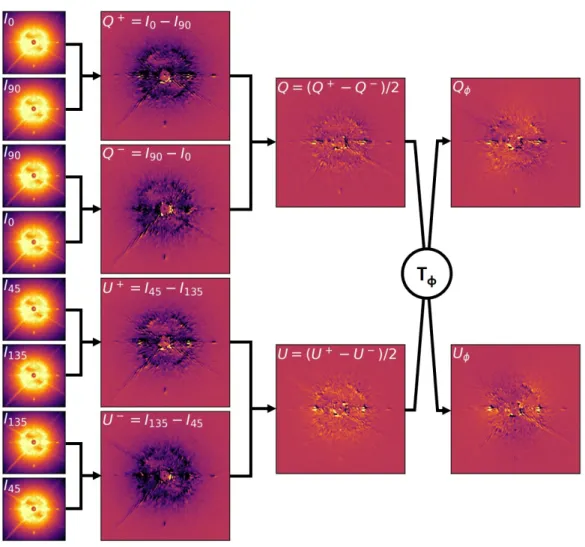
Figure 1.4: Illustration of the polarimetric differential imaging method with real data from SPHERE/ZIMPOL in the VBB filter.

detect features in the spectrum of an object that are not present in the spectrum of the star.

For example, the Hαemission produced by accretion of matter onto the surface of a planet, which can be very strong for young giant planets (Cugno et al., 2019).

This method can be extended with the use of an integral field spectrograph (IFS). An IFS allows to take resolved spectra of the environment around a star, which enables it to discern between the spectral behavior of the light from the speckles and the signal of a planet. However, with the currently available telescopes, planets that are bright enough to be directly imaged are rare or not bright enough to allow extensive studies in narrow filter bands. As a result of that, the method can rarely be applied today but it is a very promising technique for future instruments like the James Webb Space Telescope (JWST; Danielski et al. (2018)).

8

(25)

1.2.3 Polarimetric differential imaging

Polarimetry is possibly the most successful technique for suppressing the speckle noise produced by stellar light to date and is widely used for imaging of reflected light from circumstellar disks (e.g. Avenhaus et al., 2018). It relies on the fact that stellar light usually only exhibits weak linear polarization, while reflected stellar light from an object close to the star often exhibits a much larger degree of polarization. This means that removing the unpolarized fraction of the light in an image effectively suppresses the majority of the stellar light but keeps a large fraction of the scattered light, which results in a boost for the S/N of any object around a star that reflects stellar light. In practice, this is achieved by measuring the StokesI,Q andU parameters of the light by using an imaging polarimeter like the Zurich IMaging POLarimeter (ZIMPOL; Schmid et al. (2018)). The instrument effectively measures the intensity of the linearly polarized light along the position angles 0^◦, 45^◦, 90^◦and 135^◦, which are then used to calculate the Stokes parameters with:

Q=Q⁺−Q⁻

2 =(I0−I90)−(I90−I0) 2

U=U⁺−U⁻

2 =(I45−I135)−(I135−I45) 2

(1.1)

The ’+’ and ’-’ indices refer to an inversion of the instrument polarization by a half-wave plate inside the instrument. As a result of this inversion, the double difference in Eq. 1.1 removes most of the instrument polarization. This is a widely-used method in high-precision polarimeters to deal with the fraction of the linear polarization that is produced by the optical elements in the instrument itself. The technique is illustrated in Fig. 1.4 for an observation with SPHERE/ZIMPOL. More detailed information about polarimetric techniques can be found in Tinbergen (2005). TheQ andU parameters are usually transformed into the azimuthalQ_φ andU_φbasis with Eq. 1.2, whereφis the position angle with respect to the observed star.

Q_φ= −Qcos¡ 2φ¢

−Usin¡ 2φ¢ U_φ=Qsin¡

2φ¢

−Ucos¡

2φ¢ (1.2)

Since reflected light is usually polarized along the azimuthal direction,Q_φcontains the majority of the polarized signal andU_φis zero. The amplitude of the polarized signal would usually be calculated withP=p

Q²+U², however, this calculation introduces a bias into the signal for low S/N observations (Schmid et al., 2006b), because the result of this calculation is strictly positive while the noise can be either negative or positive. This problem is avoided by using Eq. 1.2, but it is important to note that usingQ_φinstead ofP can lead to discrepancies in special cases where the polarization does not strictly point in the azimuthal directionφ.

9

(26)

Most imaging polarimeters are built to so that they can record both orthogonal polarization states, e.g. I0andI90, simultaneously. This is necessary for a good suppression of the stellar PSF because of short timescale PSF variability. Polarimetry is very efficient for the suppression of unpolarized stellar light but it also introduces a few additional difficulties. For example, it can only be used to observe scattered light with a reasonably high degree of polarization, otherwise the PDI technique removes most of the scattered light as well. Other additional difficulties with polarimetry and their solutions are discussed within the scope of this thesis, including some instrumental problems which are specific to the ZIMPOL instrument.

1.3 Properties of emitted and scattered light

The two main sources of light, which are important for the direct observation are the emission of the thermal photons and the reflection of stellar light. Depending on the observed target, one of these sources of light often dominates and determines how the observations can be performed. If the temperatureT of an object is known, Wien’s displacement law (Eq. (1.3)) provides the wavelengthλmaxwhere the maximum brightness of the thermal emission for this object is located.

λmax≈2.898·10⁶nm·K

T (1.3)

This is crucial for observations in visible and near-IR, becauseλmaxis larger than 5µm for objects colder than∼600 K. This makes it almost impossible to detect thermal emission from such objects, because forλ<λmaxthe brightness decreases exponentially according to the black-body spectrum. Therefore, the thermal emission from colder objects has to be observed at longer wavelengths. However, ground based observations become increasingly more difficult at long wavelengths because of the drastically increasing IR background noise. This is why direct imaging of cold objects like circumstellar disks is preferably done by observing the reflected light at shorter wavelengths, where observations are less affected by thermal noise.

On the other hand, warm objects like young giant exoplanets are usually observed via their bright thermal emission in the near- of mid-IR, where observations are more difficult but this is more than compensated by the additional brightness of the planet.

In this section, I will discuss some of the properties of the thermal light emission and scattered light concepts that are relevant for this thesis.

1.3.1 Thermal emission

Several detections of thermal emission from exoplanets have been achieved with direct imaging from ground based telescopes in visible and near-IR wavelengths, but currently this is

10

(27)

only possible for young giant planets (e.g. Lafrenière et al., 2007a; Chauvin, 2010; Heinze et al., 2010; Rameau et al., 2013b; Biller et al., 2013; Nielsen et al., 2013; Wahhaj et al., 2013;

Chauvin et al., 2015; Meshkat et al., 2015; Reggiani et al., 2016), because they can be very bright and self-luminous from the still ongoing formation process. Planets with temperatures far exceeding∼1000 K have been found in the past, for example in the case of the giant planet βPictoris b (Lagrange et al., 2009b), which places the maximum of its thermal emission (see Eq. 1.3) at a wavelength that can still comfortably be observed with ground based telescopes.

However, surveys in recent years have concluded that giant planets in general are not common (e.g. Fressin et al., 2013) and the nearest star forming regions, which contain young stars and exoplanets, are located relatively far away from the sun (100-200 pc). This has severely limited the number of direct detections so far.

Direct imaging of thermal emission from older, evolved planets is nearly impossible for instruments and telescopes that exist today because of their low temperatures. Using the energy equilibrium of the stellar irradiation and assuming that the planet re-emits the energy like a black-body allows to calculate its equilibrium temperatureTequwith Eq. 1.4 (Traub et al., 2010).

Tequ=

µ1−AB

4f

¶1/4

³rS

d

´1/2

TS (1.4)

This is a rough estimate for the effective temperature of a planet with Bond AlbedoAB at a separationdfrom a star with stellar radiusrSand temperatureTS. The parameterf describes the re-distribution of heat on the planet surface. For effective heat re-distributionf is equal to 1 and for tidally locked planetsf is roughly∼0.5. This formula provides a very good estimate for the temperatures of almost all solar system planets. Only the giant planets outside of Saturn have effective temperatures slight aboveTequbecause they still have non-negligible internal heat sources (Traub et al., 2010). From Eq. 1.4 we learn that an evolved planet needs to be located closer than∼0.15AU²to a solar type star to exhibit a temperature of 600 K and therefore barely be observable from its thermal emission alone. Even if such a planet would be located around a star at a distance of only 1 pc, the angular separation from its host star in combination with its low brightness would be too small to allow a detection with any instrument that exist today.

The solution to this problem lies in the construction of extremely large telescopes like the ELT (Kasper et al., 2010; Keller et al., 2010), which would allow to observe at a significantly better resolution and in the construction of large aperture, space-based observatories. Large space- based instruments like HabEx (Gaudi et al., 2020) or the Origins Space Telescope (Staguhn et al., 2019), which could be built in the future, have the advantage of lower thermal background noise at long wavelengths due to the absence of Earth’s atmosphere and therefore have a

2Assumingf=1 andA_B=0.5

11

(28)

natural advantage for the search cold evolved exoplanets.

1.3.2 Scattered light

For the interpretation of scattered light from an object, it important to consider a few basic principles, which govern the scattering process, because the scattered light depends strongly on the dominating scattering processes at the particular wavelength of the observations. More general studies of this subject can be found for example in the books from van de Hulst (1980) and Bohren and Huffman (1983), which were used as a source for the explanations in this work.

On a macroscopic scale, scattered light can behave very differently depending on the sizeaof the object that scatters the light, and also its surface properties and composition. Especially important is the size of the particle with respect to the scattered wavelength. Therefore, different scattering regimes are usually identified with the dimension-less size parameterx:

x=2πa

λ (1.5)

The exact calculation of the scattering solution for an electromagnetic plane wave that scatters on a complex particle is numerically very challenging. However, for certain regimes there are approximations which can simplify the calculations significantly. For very small particlesx¿ 1, scattering is dominated by the Rayleigh mechanism, which has a simple analytical solution.

Scattering on larger particles with sizes similar to the wavelengthx≈1 or large particles withxÀ1 is often calculated with the Mie theory or with discrete dipole approximation (DDA; Zubko et al. (2009)) and effective medium theory (EMT) for objects with complicated structures.

Basic principles

Monochromatic light at a sufficiently large distance from the source can be modeled as an electromagnetic plane wave with an electric field determined by:

E(r,t)=E₀e^{i(k r}^−ω^t) (1.6)

For simplicity it can be assumed that the wave propagates in z-direction and oscillates in the x-y plane. The wave vector then reduces tok=^2π_λ ez. The frequency of the light isν=_2π^ω and the amplitude isE0=E0,xex+E0,yey. This model for a plane wave assumes implicitly that the light is not circularly polarized, which is a reasonable assumption for all applications discussed here.

12

(29)

The thermal emission from a sufficiently homogeneous and spherical body like a star is largely unpolarized. This does not apply to a single plane wave or photon, since single photons are always polarized, but to the collection of all emitted photons. Thermal emission of a star, for example, produces photons with randomly oriented linear polarization, therefore the average polarization of all photons is zero. In astronomy, light is often said to be unpolarized or partially polarized, which refers to the average direction of the linear polarization from photons collected from a source over a sufficiently long time. Unpolarized light can then become partially linearly polarized due to anisotropic effects like scattering or by being emitted by an anisotropic body. This is the basis on which polarimetric differential imaging is built upon.

For the analysis of light scattering processes, it is useful to separate the electromagnetic wave of the incident light into two components withEi=E_⊥e_⊥+E_∥e_∥. This separation treats the incident waveEi as a superposition of the part of the wave which is perpendicular to the scattering planeE_⊥e_⊥and the part which is parallel to the scattering planeE_∥e_∥. The relation between the incident waveEiand the scattered waveEscthen simplifies to

ÃE_∥sc

E_⊥sc

!

=e^{i k(r−z)}

−i kr

ÃS2 S3

S₄ S₁

! ÃE_∥i

E_⊥i

!

(1.7)

for an incident waveEitraveling in z-direction and a scattered waveEsc observed at a large distancekrÀ1 from the light scattering particle or body (see Bohren and Huffman (1983)).

The entriesS_1..4 of the scattering matrix depend on the scattering angle and the particle properties. The scattering angle θis defined as the angle between the scattered and the incident wave∠^(Esc,Ei). In this work I useθ=0^◦for forward scattering andθ=180^◦for backward scattering. This definition is common in the literature related to exoplanets and circumstellar disks, but the reverse definition is used as well in literature concerning interstellar dust and interplanetary dust inside the Solar System.

CCD detectors in cameras only measure what is usually referred to as the intensity of the light or the StokesI parameter, which can be calculated asI= |E|². Polarimeters then use linear polarizers or equivalent optical elements upstream of the detector, which allows to measure the intensity along certain axis and subsequently the construction of the other Stokes parameters withQ=I₀◦−I₉₀◦andU=I₄₅◦−I₁₃₅◦. The circular polarization, represented by the StokesV parameter can be neglected in the applications of this work, therefore the amplitude of the polarized intensity is given byP=p

Q²+U².

The intensity of the scattered waveIscis proportional to the scattering cross-sectionσscand

13

(30)

the scattering phase functionp_sc(θ,φ) (SPF):

Isc∝σscpsc(θ,φ) (1.8)

The SPF describes the amount of light, which is scattered into a unit solid angle for each direction and is therefore a normalized distribution function with

Z

θpsc(θ,φ)dΩ=1 (1.9)

Since scattering discussed in this work happens on distributions of particles that are not aligned or extended in preferred directions, the SPF only depends on the scattering angleθ, and the normalization can be rewritten as:

2πZ _π

0

p_sc(θ) sinθdθ=1 (1.10)

Diffraction effects can result in complex shaped SPFs, especially if the size of the particles that scatter the light and the wavelength of the scattered light are of similar order (x≈1). However, for simplicity, SPFs are often classified according to their preferred scattering angles by using the asymmetry parameterg. The asymmetry parameter is defined as the average cosine of the scattering angle with:

g= 〈cosθ〉 =Z

4πp_sc(θ) cosθdΩ (1.11)

The asymmetry parameter is zero ifpsc(θ) is symmetric atθ=90^◦, i.e. forward and backward scattering show the same behavior. If the majority of the light is scattered toward the forward direction,g is positive andg is negative if the majority of the light is scattered toward the backward direction.

The polarized intensityP(θ) of the reflected light is proportional to the scattered light intensity I_scand the fractional polarizationp_pol(θ):

P(θ)=p_pol(θ)Isc (1.12)

14

(31)

The fractional polarizationp_pol(θ) describes the scattering angle dependency of the polarized intensity amplitudeP(θ) and also depends only on the scattering angleθ as long as the scattering particles are not aligned in any preferred direction. In this work,p_pol(θ) will be either referred to as the degree of polarization or the fractional polarization.

In the same way, that the angle dependency of the scattered light intensityI_scis described by the SPF, the polarized intensityP(θ) is described by the polarized scattering phase function (pSPF), which is defined by the combination of the SPF and the fractional polarizationpsc(θ)· p_pol(θ). For symmetry reasons, the fractional polarization for forward scattering (θ=0^◦) and backward scattering (θ=180^◦) is always zero. The scattering angleθmax, which refers to the angle where the polarization of the scattered light reaches its maximum polarizationpmax, is usually located around 90^◦, while the direction of the polarization is oriented parallel to the scattering planee_∥.

Scattering phase functions

Light scattering on polarizablesmall particles(x¿1) is described by the Rayleigh scattering approximation. Rayleigh scattering assumes that the electromagnetic waves of the light induce an electric field into the particles that turns them into small oscillating dipoles. The particles then oscillate with the frequency of the incident radiation and therefore re-emit radiation with an identical frequency, which results in an elastic scattering process. Rayleigh scattering is one of the few physical models for which a solution for the SPF can be calculated analytically:

IRa y∝λ⁻⁴(1+cos²θ) (1.13)

The cross-sectionσscfor Rayleigh scattering is inverse proportional to the fourth power of the scattered wavelengthλ. As a result of that, Rayleigh scattering particles are said to be blue, because they scatter blue light much more efficiently than red light. The SPF for Rayleigh scattering is shown in Fig. 1.6(a) along with a few other examples, it is proportional to (1+cos²θ) and therefore slightly anisotropic with light being scattered preferentially in the forward and backward direction. Even though Rayleigh scattering is not isotropic, the asymmetry factorgis equal to zero because forward and backward scattering behavior are identical.

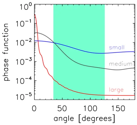
Light scattering onmedium sized particles(x≈1−10) is often calculated with Mie theory (Mie, 1908). Mie theory describes the exact solution of Maxwell’s equation for scattering on spherical particles. It is frequently used, for example, to calculate light scattered by particles in circumstellar disks (e.g. Mulders et al., 2013; Perez et al., 2015; Marino et al., 2015; Price et al., 2018). The main advantage of this theory is its simplicity, since the only free parameter is the particle size. As a result of that, the exact solution to the scattering process is not excessively expensive to calculate numerically. Fig. 1.5 shows a few examples of SPFs for Mie scattering on 15

(32)

Figure 1.5: Solutions for the SPF of dust particles with different sizes, calculated with Mie theory (Source: Mulders et al. (2013)).

particles with different sizes with respect to the scattered wavelength. The different SPFs show that Mie scattering is characterized by a forward scattering peak, which grows increasingly stronger with larger particle sizes.

The forward scattering peak is a result of diffraction, with the forward peak corresponding to the "zero-order mode" of the diffraction pattern. Higher order modes are usually visible as well (see Fig. 1.5, large particle size) for scattering with one single size parameterx, but are in reality washed out due to the presence of particles with different sizes and due to observations being performed in broad-band filters. Mie theory is often used because of its simplicity but increasingly accurate measurements have revealed that the results often do not match with the observed phase functions for astrophysical dust (e.g. Pinte et al., 2008; Perrin et al., 2009). As a result of that, the micron sized dust in circumstellar disks is expected not consist of compact particles, but rather dust aggregates with potentially high porosity, which is caused by coagulation of smaller dust grains (e.g. Beckwith et al., 2000; Dominik et al., 2007; Natta et al., 2007). This causes "fluffy" particle morphologies that are very different from the compact spheres assumed in the Mie theory. Scattering solutions for porous aggregates have been calculated using effective medium theory (EMT) and discrete dipole approximation (DDA;

Zubko et al. (2009)), which are more computationally expensive but have shown to reproduce the observed signals more accurately than Mie theory (e.g. Pinte et al., 2008).

16

(33)

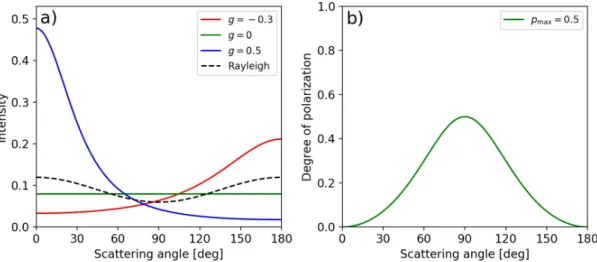
Figure 1.6: (a) A few examples of SPFs calculated with the Henyey-Greenstein function (solid lines) compared to the PSF that results from Rayleigh scattering (dashed line). Positivegvalues result in forward scattering with a maximum atθ=0^◦and negativegvalues result in backward scattering with a maximum atθ=180^◦. (b) The angle dependent fractional polarization as derived for Rayleigh scattering but with the maximum polarizationpmaxatθ=90^◦set to a value of 0.5.

The continuation for the scattering response oflarge particles(xÀ1) is described by geomet- ric optics. The SPF in this regime is characterized by a large but extremely narrow diffraction peak in the forward direction and some amount of backward scattering, which is caused by the illumination of the large particles (Min et al., 2010). This behavior is similar to the reflected light intensity observed for the Moon or other large Solar System bodies at different phases.

Even large bodies like the Moon exhibit diffraction, which scatters a large amount of light in the forward direction, but with a diffraction peak so narrow that it is only visible for scattering angles very close to 0^◦.

For simple model calculations it is often unreasonable to calculate complex SPFs, especially if the properties of the simulated material are not well known. In such cases, it is more practical to use an analytic approximation that can be tuned to have a similar angular dependency as expected for a real SPF. The Henyey-Greenstein (HG) function (Henyey and Greenstein, 1941) is such a convenient 1-parameter phase function of the form:

p_HG(θ,g)= 1 4π

1−g²

(1+g²−2gcosθ)^3/2 (1.14)

Its only free parametergallows to change the asymmetry of the distribution between isotropic scattering forg=0, forward scattering for 1>g>0 and backward scattering for−1<g<0.

Fig. 1.6(a) shows examples for HG functions compared to the Rayleigh SPF, which also has 17

(34)

an asymmetry parameter ofg=0 but is not part of the HG functions. The HG functions are widely used to model the angular distribution of scattered light in circumstellar disks and are simple and decent models for the forward scattering dust grains that can be found in debris disks (e.g. Engler et al., 2017, 2018; Milli et al., 2019).

Angle dependent fractional polarization

The angle dependent fractional polarizationppol(θ) describes the degree of polarization of scattered light at different scattering angles and it can be determined byp_pol(θ)=P(θ)/Isc(θ) after measuring the angle dependent polarized intensityP(θ)≈Q_φand total intensityI_sc(θ) of the scattered light. For a pure Rayleigh scattering material, it is again possible to determine the solution for the fractional polarization analytically:

p_pol(θ)=1−cos²θ

1+cos²θ (1.15)

The maximum degree of polarizationpmaxfor Rayleigh scattering is located at a scattering angle of exactly 90^◦withpmaxequal to 100%. Since the fractional polarization for Rayleigh scattering is simple, analytically determined and its angle dependence shows the typical features of many of the more complex materials, it can be used as a decent approximation for a material with unknown composition (e.g. Engler et al., 2017, 2018; Milli et al., 2019). For that purpose, Equ. 1.15 is usually additionally multiplied by a free parameterpmaxto account for the fact that most materials produce much less than 100% maximum polarization. An example of such a Rayleigh like fractional polarization withp_max=0.5 is shown in Fig. 1.6(b).

The fractional polarization caused by light scattering other materials has also been calculated with Mie theory in the past but comparisons with measurements have shown that the often measured high polarizations (∼30%) in combination with the observed, relatively large particle sizes (∼1µm) are often not compatible with the low polarization prediced by Mie theory.

Solutions have been proposed that involve again the presence of porous aggregate particles (Pinte et al., 2008; Perrin et al., 2009). Calculations have shown that such large particles in combination with sufficiently high porosity can produce high maximum polarization levels, because light is then effectively scattered by smaller scale structures of the large particles.

The fractional polarization is a useful parameter because it provides additional information about the optical properties of the light scattering material, but also because it is a normalized quantity. Being a normalized quantity means that the degree of polarization, other than absolute quantities likeP(θ) and I_sc(θ), is independent on many parameters that can be difficult to determine for an astronomical object, like the density of the observed material.

The downside is, that bothP(θ) andIsc(θ) have to be measured for an object, which is often difficult for for objects outside the Solar System due to instrumental limitations but have been

18

(35)

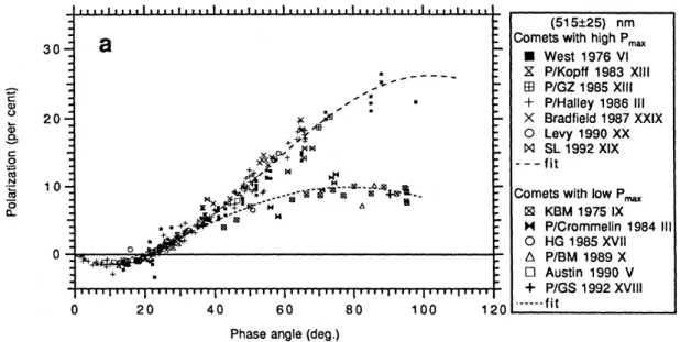
Figure 1.7: Measurements for the fractional polarization of light reflected by cometary dust at different scattering angles at visible wavelengths. The phase angle in this plot was defined so that 0^◦corresponds to backward instead of forward scattering. The polarization measurements reveal a negative backward scattering branch at small phase angles. Negative polarization means that the polarization of the scattered light is oriented perpendicular to the scattering plane instead of parallel, which is considered the usual orientation. (Source: Levasseur- Regourd et al. (1996))

successfully achieved a small number of times (Canovas et al., 2013; Avenhaus et al., 2014).

However, precise measurements of the fractional polarization for circumstellar disks are still rare because of this difficulty. Modern instruments with PDI capabilities have allowed do determine partial pSPFs of certain disks (e.g. Milli et al., 2017, 2019) but the simultaneous measurement of the SPF is complicated by the fact that separating the disk signal from the bright star (e.g. with ADI) often introduces large systematic measurement errors. For determining a phase function, it is also important that the reflected light can be measured for a large range of different scattering angles, which is only possible for circumstellar disks that are sufficiently inclined with respect to the line of sight. Even then, scattering angles close to 0^◦and 180^◦are inaccessible for observations of scattered light outside of the Solar System because they coincide with the observed star being directly behind or in front of the light scattering material, respectively. More intensive studies have been done on the optical properties of cometary dust particles within the Solar System. Comets are suspected to be remnants of the early Solar System and are therefore expected to show properties similar to the dust found in the disks around young stellar systems. Fig. 1.7 shows a series of measurements of the angle dependent fractional polarization for different comets. Some of which show a relatively highpmaxthat was also found in measurements of certain circumstellar disk. More importantly, extensive analysis of the angle dependent fractional polarization for cometary dust (e.g. Zubko et al., 2014) have shown that it exhibits various features which can be used as 19