Abstract
Gravitational sinking of photosyntheticallyfixed particulate organic carbon (POC) constitutes a key component of the biological carbon pump. The fraction of POC leaving the surface ocean depends on POC sinking velocity (SV) and remineralization rate (Cremin), both of which depend on plankton community structure. However, the key drivers in plankton communities controlling SV andCreminare poorly constrained. In fall 2014, we conducted a 6‐week mesocosm experiment in the subtropical NE Atlantic Ocean to study the influence of plankton community structure on SV andCremin. Oligotrophic conditions prevailed for thefirst 3 weeks, until nutrient‐rich deep water injected into all mesocosms stimulated diatom blooms. SV declined steadily over the course of the experiment due to decreasing CaCO3ballast and—according to an optical proxy proposed herein—due to increasing aggregate porosity mostly during an aggregation event after the diatom bloom. Furthermore, SV was positively correlated with the contribution of picophytoplankton to the total phytoplankton biomass.Creminwas highest during a Synechococcusbloom under oligotrophic conditions and in some mesocosms during the diatom bloom after the deep water addition, while it was particularly low during harmful algal blooms. The temporal changes were considerably larger inCremin(max.fifteenfold) than in SV (max. threefold). Accordingly, estimated POC transfer efficiency to 1,000 m was mainly dependent on how the plankton community structure affectedCremin. Our approach revealed key players and interactions in the plankton food web influencing POC export efficiency thereby improving our mechanistic understanding of the biological carbon pump.
1. Introduction
Phytoplanktonfix approximately 50‐Gt carbon per year, which is comparable to the annual primary produc- tion of the terrestrial biosphere (Field et al., 1998; Longhurst et al., 1995). The majority of the organic biomass generated by phytoplankton is consumed and remineralized in the surface ocean, while 11–27%
is exported below the euphotic zone (Field et al., 1998; Henson et al., 2011). This exportflux maintains a permanent surface‐to‐depth CO2gradient, which allows the ocean to store significantly more atmospheric CO2than it would without this biological carbon pump (BCP; Volk & Hoffert, 1985). The BCP is driven by (1) gravitational sinking of particulate organic carbon (POC), (2) downwelling of POC and dissolved organic carbon (DOC), and (3) zooplankton‐mediated active transport (Ducklow et al., 2001; Hansell &
Carlson, 2001; Steinberg et al., 2008). Among these mechanisms, gravitational sinking is considered the most important pathway, although this is still a matter of debate (Boyd et al., 2019; Hernández‐León et al., 2019;
Steinberg & Landry, 2017; Stukel et al., 2018).
The efficiency of the BCP through gravitational sinking can be determined empirically byfitting a power law function to, for example, depth‐resolved sediment trapfluxes (Martin et al., 1987). This provides thebvalue, which quantifies the transfer efficiency from the surface to the deep ocean. However, it is also possible to determine BCP efficiency mechanistically by assessing the ratio of carbon‐specific remineralization rates (Creminin d−1) and particle sinking velocity (SV in m d−1; Sanders et al., 2014). This ratio is known as the remineralization length scale (RLS in m−1) and quantifies the fraction of carbon within an aggregate that is remineralized per meter sinking (e.g., Belcher et al., 2016; Iversen et al., 2010). Densely packed and heavily ballasted particles will sink rapidly and provide relatively little surface area for bacterial remineralization
©2019. The Authors.
This is an open access article under the terms of the Creative Commons Attribution License, which permits use, distribution and reproduction in any medium, provided the original work is properly cited.
a considerably larger influence on particle remineralization rate than on sinking velocity
Supporting Information:
•Supporting Information S1
Correspondence to:
L. T. Bach,
lennart.bach@utas.edu.au
Citation:
Bach, L. T., Stange, P., Taucher, J., Achterberg, E. P., Algueró‐Muñiz, M., Horn, H., et al. (2019). The influence of plankton community structure on sinking velocity and remineralization rate of marine aggregates.Global Biogeochemical Cycles,33, 971–994, 971–994. https://doi.org/10.1029/
2019GB006256
Received 14 APR 2019 Accepted 25 JUL 2019
Accepted article online 1 AUG 2019 Published online 12 AUG 2019
(low RLS). Conversely,fluffy aggregates with plentiful easily degradable organic matter will sink slowly and be largely decomposed before they reach depths below the winter mixed layer (high RLS; Francois et al., 2002). Assessing the fraction of POC transferred below winter mixed layer depth is important because par- ticles that successfully carry POC down there will likely lock CO2in water masses, which have no exchange with the atmosphere for centuries to millennia (Kwon et al., 2009). Both SV andCreminare determined by surface ocean plankton communities as they form the sinking POC and set its initial properties although SV andCreminare modified in deeper water (Fischer & Karakaş, 2009; Henson, Sanders, et al., 2012; Lam et al., 2011; Laurenceau‐Cornec et al., 2015; Lomas et al., 2010).
Observations based on sediment trap deployments led to the hypothesis that the availability of ballast miner- als largely controls the transfer of POC through the mesopelagic (Armstrong et al., 2002; Francois et al., 2002; Klaas & Archer, 2002). However, more recent assessments of sediment trap data challenged theballast ratio hypothesis(Armstrong et al., 2009) by indicating that the global correlation between ballast and POC fluxes is an artifact of the large degree of spatial averaging (Wilson et al., 2012). Deviations from this correla- tion exist regionally, indicating that ballast can be very important under certain conditions but other factors such as particle (re)packaging and POC refractiveness against remineralization should also be taken into account to fully understand regionally and temporally changing patterns of CO2sequestration efficiency through gravitational sinking (Boyd & Trull, 2007; Le Moigne et al., 2016; Passow & De La Rocha, 2006;
Wilson et al., 2012). Particle properties that determine SV andCreminare largely controlled by the plankton community, and therefore, it is essential to understand the ecological processes that form and reprocess sink- ing POC (Bach et al., 2016; Henson, Lampitt, et al., 2012; Herndl & Reinthaler, 2013; De La Rocha & Passow, 2007; Lam et al., 2011; Lam & Bishop, 2007; Siegel et al., 2014).
However, investigating the links between surface ocean plankton communities and POC exported to depth faces several problems. These are primarily related to the lateral advection of POC during sinking and the time lag between primary production and export. Both must be taken into account to correctly link particles collected at depth with the plankton communities that actually produced them (Henson et al., 2015;
Prahl et al., 2000; Stange et al., 2017). In situ mesocosms have been suggested as an important tool to overcome the spatial and temporal challenges associated with oceanic sampling (Bach et al., 2016;
Legendre et al., 2018; Sanders et al., 2014). Although mesocosms largely exclude the physical complexity of the marine realm, they enclose the same plankton communities for long times and therefore simulate a Lagrangian system. This allows us to link processes in the plankton community with export‐relevant para- meters without the ambiguity caused by unconstrained advection or unknown time lags. Indeed, previous in situ mesocosm experiments have proven to be useful for this purpose (Bach et al., 2016; Bressac et al., 2014;
Gazeau et al., 2017; Knapp et al., 2016; Stange et al., 2018).
In a recent in situ mesocosm experiment at the Norwegian coast, we investigated the influence of processes in the plankton community on SV (Bach et al., 2016). We found that enhanced ballasting of particulate organic matter by minerals did not necessarily lead to faster sinking of particles. Instead, aggregate porosity played an equally important role, which in turn was dependent on the trophic state of the food web. These results support the notion that plankton community structure is important in controlling SV. However, SV is only one side of the coin and to assess the influence of plankton on BCP efficiency, it is essential to measure SV andCreminsimultaneously. We therefore conducted an in situ mesocosm experiment in the oligotrophic NE Atlantic where these two measurements and a detailed examination of the plankton community were combined.
2. Material and Methods
2.1. Experimental Design
On 29 September 2014, we deployed nine units of the Kiel Off‐Shore Mesocosms for Future Ocean Simulations (M1–M9; Riebesell et al., 2013) in Gando Bay, Gran Canaria (27°55′41″N, 15°21′55″W). The mesocosms consisted of a cylindrical bag made of transparent polyurethane foil (13 m long, 2 m in diameter), which was suspended in an 8‐m highfloatation frame. Each bag was equipped with a 2‐m‐long funnel‐
shaped sediment trap (Boxhammer et al., 2016).
lating the water mass. This marked the beginning of the experiment.
Between days 0–6 and on days 21 and 38, seven of the nine mesocosm units were enriched with CO2aerated seawater to reachpCO2values of 369, 352 (M1 and M9 both untreated control mesocosms), 563 (M3), 668 (M7), 716 (M4), 887 (M2), and 1,025 (M8)μatm. The influence ofpCO2on SV andCreminwas not further explored in our analyses because of three reasons. First, our initial data exploration indicated no clear CO2
effect. Second,pCO2cannot influence SV directly because sinking is a physical process, although it can influ- ence SV by changing plankton communities (Bach et al., 2016). Third,Cremincan be influenced directly by pCO2by changing metabolic rates of heterotrophs (Piontek et al., 2010) but also by changing plankton com- munities (Stange et al., 2018). Our setup does not allow us to distinguish thisphysiologicalfrom theecological component, but we would expect a much more consistent CO2dependency if physiology had been the domi- nant factor. We therefore focus in this paper on the links between plankton communities and SV andCremin
as they seem to be more important, and thefindings are also applicable in a more general context (such as coupling ecological processes with exportfluxes). Please note, however, that we investigated the influence of pCO2on export massfluxes and organic matter stoichiometry in a separate paper (Stange et al., 2018).
On day 23 we collected ~85 m3of natural nutrient‐rich seawater from a depth of 650 m with a specifically designeddeep water collection bag. The bag was lowered to the target depth at a location 4 nautical miles off- shore Gran Canaria, where the ocean is ~1,000‐m deep, andfilled with a remote‐controlled propeller system.
Once the bag was full, a 300‐kg weight was released so thatfloatation panels mounted at the top of the bag brought it back to the surface. Afterward, the bag was gently towed to the mesocosm deployment site with the vessel SAPCAN IV and moored next to the mesocosms. About 20% (~7 m3) of the water was pumped out from each mesocosm and replaced with deep water, which was injected evenly into the water columns of the mesocosms with a specifically designed distribution device during the night from day 24 to 25. Please note that mesocosm 6 was irreparably damaged on day 26 and therefore only included in the analyses until that day. A detailed description of all technical operations is provided in the overview paper accompanying this mesocosm campaign (Taucher et al., 2017).
2.2. Sampling and Sample Processing of Water Column Parameters
Suspended particulate material and nutrients in the mesocosm water columns were sampled with two dif- ferent devices every other day between 09:00 a.m. and 12:00 p.m. from small boats. Chlorophylla(chl‐a), PM, and phytoplankton were sampled with a specifically designed vacuum pumping system, which effi- ciently collected equal amounts of water from each depth between 0 and 13 m (Taucher et al., 2017).
Nutrient and microzooplankton samples were collected with depth‐integrating water samplers (IWSs, Hydro‐Bios, Kiel). The IWSs are equipped with pressure sensors and gently take in a total volume of 5 L uni- formly distributed over 0–13 m.
Seawater collected with the vacuum system was stored in 20‐L carboys and transferred into a temperature‐ controlled room (set to 15 °C) immediately after arriving at the land‐based laboratory facilities of Plataforma Oceánica de Canarias (PLOCAN), which is located next to Taliarte harbor and hosted our study. The 20‐L carboys were gently mixed before taking subsamples for the individual measurements. Subsamples for chl‐a and POC were filtered (Δpressure = 200 mbar) on glass fiber filters (GF/F nominal pore size = 0.7μm). Chl‐asamples were immediately frozen to−80 °C and later analyzed using reverse‐phase high‐ performance liquid chromatography following van Heukelem and Thomas (2001). POCfilters were stored in glass Petri dishes and immediately frozen to−20 °C afterfiltration. POC samples were fumed in hydro- chloric acid (37%) for 2 hr before measurement. POC concentrations were determined using an elemental analyzer (EuroEA) following Sharp (1974). Flow cytometry subsamples were taken directly from the 20‐L
carboys and measured within 3 hr using an Accuri C6flow cytometer (BD Biosciences). Gates were set based on the forward scatter (FSC‐A) and redfluorescence (FL3‐A) signals except for theSynechococcusgroup where the orange (FL2‐H) instead of FL3‐A signal was used to distinguish them from bulk phytoplankton.
The size of different phytoplankton groups was determined by fractionation with a variety of polycarbonate filters (0.2, 0.8, 2, 3, 5, and 8μm) following Veldhuis and Kraay (2000). We distinguished between picoeukar- yotes (Peuks; 0.2−2μm),Synechococcus‐like autotrophs (Synechococcus; 0.6−2μm), small nanoautotrophs (Nano I; 2−5μm), larger nanoautotrophs (Nano II; 5−8μm), and microautotrophs (Micro; >8μm). We then calculated the relative redfluorescence contribution of each of these groups to the total redfluorescence as described by Bach et al. (2018). A significant linear correlation between FL3‐A and chl‐a concentration confirmed that the redfluorescence measurement is a useful proxy for chl‐a(Figure S1 in the supporting information). Accordingly, FL3‐A was converted to chl‐aand used thereafter to calculate the percentage each of the above mentioned groups contributed to the total chl‐aconcentration. Samples for transparent exopolymer particles (TEP) werefiltered onto polycarbonatefilters (0.4‐μm pore size) and subsequently stained with Alcian Blue (Passow & Alldredge, 1995). TEP concentrations were determined colorimetrically with a spectrophotometer through absorption at 787 nm. The dye solution had previously been calibrated using Gum Xanthan, and the concentrations of TEP are expressed as microgram Gum Xanthan equivalents per liter (μg GXeqL−1).
IWS microzooplankton samples were transferred into brown glass bottles (250 ml), preserved with acidic Lugol's solution (1–2%final concentration), and stored in the dark until measurement. Abundances of the major groups, that is, ciliates and heterotrophic dinoflagellates, were determined using a Zeiss Axiovert 25 inverse light microscope (Utermöhl, 1958). Seawater collected with the IWS for nutrients were transferred into acid‐cleaned (10% HCl) plastic bottles (Series 310 PETG) andfiltered using 0.45‐μmfilters (cellulose acetate, Whatman) directly after arrival at PLOCAN. NO3−+ NO2−(NOx−), Si (OH)4, and PO43−concentra- tions were determined photometrically (Hansen & Koroleff, 1999; Murphy & Riley, 1962), while NH4+
con- centrations were determined fluorometrically (Holmes et al., 1999). The applied analytical tools and specifications to analytical procedures are described with more detail by Taucher et al. (2017).
Mesozooplankton samples were collected every eighth day (2 to 4 p.m. local time) with vertical net hauls using an Apstein net (55‐μm mesh size, 17‐cm diameter opening) equipped with a closed cod end. The sam- pling depth was restricted to 13 m to avoid contact of the net with the sediment trap material accumulating at the bottom of the mesocosms. Samples were rinsed on board the sampling boats, collected in containers, and stored in cool boxes until arrival at PLOCAN. Back in the laboratories, samples were preserved in dena- tured ethanol and quantified and classified to the lowest possible taxonomic level using a stereomicroscope (Olympus SZX9) as described by Algueró‐Muñiz et al. (2019)
In situ sizes of aggregates were measured inside the mesocosms with vertical casts of the profiling under- water camera system KIELVISION (Taucher et al., 2018). The camera is equipped with a 12 megapixel sen- sor, has a resolution of 25μm per pixel, and photographs a volume of 120 ml per picture. Camera profiles were obtained by manually lowering the system at∼0.5 m/s and recording images from downcasts only.
Image acquisition was triggered by an integrated pressure sensor, which was set to obtain one image frame per 0.1‐m depth interval, resulting in a total sample volume of∼13–14 L per mesocosm profile. A detailed description of the camera system and the evaluation procedures is provided in the paper by Taucher, Arístegui, et al. (2018).
2.3. Sampling and Processing of Sedimented Particulate Organic Matter
Particulate matter (PM) that settled into the terminal sediment traps at the bottom of the mesocosms was recovered every other day between 08:00 and 09:00 a.m. with the vacuum method described by Boxhammer et al. (2016). Briefly, the collection cylinder at the bottom of the sediment trap was connected to the surface with silicon hose. By applying a weak vacuum to the hose, we sucked all material accumulated in the sediment traps up to the surface and collected this in 5‐L glass bottles (Schott Duran). The bottles were stored in cool boxesfilled with seawater until arrival in the laboratories at PLOCAN in the early afternoon.
Back on shore, we homogenized the samples by gently rotating the glass bottles and took a 60‐ml subsample (1–5% of the total sample) with a serological pipette for the determination of SV andCremin(see sections 2.4 and 2.5). The remaining particle suspension was concentrated by centrifugation, freeze‐dried, and ground with a ball mill to transform the sample into a homogenous powder (Boxhammer et al., 2016). Total
transferred into 40‐ml plastic vials and heated for 135 min with NaOH (0.1 M) at 85 °C. Subsequently, sam- ples were neutralized using H2SO4(0.05 Molar) and analyzed spectrophotometrically following Hansen and Koroleff (1999).
We typically report PM massflux to the sediment trap inμmol/L per 48 hr (Gmeasured) as this value is useful to calculate elemental budgets and can be easily calculated from known PM massflux to the sediment traps and mesocosm volumes (Boxhammer et al., 2018). Here, we report PM massflux in mmol/m2per 48 hr (Gcor) as this is more easily comparable to the sediment trap and thorium literature (Buesseler, 1998;
Honjo et al., 2008). The problem here is that the mesocosm volume varied between 30.8 and 36.8 m3because of theflexible nature of the bags even though the diameter of the stabilizing rings was identical (2 m). Thus, to correct the massflux, we had to normalize the measured massflux to the average mesocosm volume (Vaverage) as
Gcor¼Gmeasured×Vmesocosm×Vmesocosm
Vaverage =πr2 (1)
whereVmesocosmare the individual volumes of the nine mesocosms determined as described by Taucher et al. (2017) and r is the radius of the cylindrical mesocosm bags (1 m).
2.4. Measurement of Carbon‐Specific Remineralization Rates (Cremin)
Seawater used for dissolved oxygen (O2) consumption assays was collected from each mesocosm with IWS hauls on days 11, 19, 23, 29, 33, 37, 41, 47, and 53. Samples from each mesocosm werefilled headspace‐free (allowing significant overflow) into seven 250‐ml Schott Duran bottles. No mesh was applied during thefill- ing procedure. The 63 bottles per sampling day were stored in dark plastic boxes and covered with aluminum foil inside cool boxes. Upon arrival in the laboratory (~3–6 hr after taking the samples), all bottles were trans- ferred into a water bath at in situ temperature (22 °C) and stored there in the dark for max. 2 hr until the incubation assays started.
To initiate the incubations, we added 1–3 ml of the PM suspension collected in sediment traps into four of the seven bottles per mesocosm. Unlike in previous experiments (e.g., Bach et al., 2016), the suspension was homogeneous so that 1–3 ml were representative for the bulk sample. The three remaining bottles per mesocosms were not enriched with sediment trap material and served as blank incubations to correct for the O2consumption in the natural unfiltered seawater. Care was taken to exclude air bubbles from the incubations. All bottles were placed on a slowly rotating plankton wheel (~1 rpm) and incubated in the dark for up to 39 hr in a temperature‐controlled room set to the in situ temperature (22 °C) of surface water (0–15 m) in Gando Bay.
O2consumption inside the bottles was measured using noninvasive O2sensitive microsensor spots (PSt3‐ NAU spots, PreSens) mounted with silicon glue inside the 250‐ml incubation bottles. The applied sensor spots were two‐point calibrated with air‐saturated and anoxic water. They had a measurement range of 0–1,400μmol/L O2, a resolution of ±1.4μmol/L O2at 283μmol/L O2, and a response time of <40 s. The O2concentrations were read 6–7 times during each incubation through the glass walls of the bottles using a handheld optical O2meter (Fibox 4, PreSens, Germany). Thefirst measurement was always conducted immediately after the addition of PM to the replicate bottles. The second measurement was taken approxi- mately 2 hr after the start to have a second measurement early during the assay. Subsequent measurements were performed in 8‐hr intervals. The Fibox4 handheld O2meter automatically corrects for salinity and tem- perature. We used the daily average salinity determined with a conductivity, temperature, depth (CTD)
probe on the day of incubation (Taucher et al., 2017). Temperature was measured in a dummy bottle that was treated similar to the incubation bottles.
After the incubation period, the entire content of the bottles wasfiltered (Δpressure = 200 mbar) onto com- busted glassfiberfilters (pore size 0.7, GF/F, Whatman). Allfilters were fumed with hydrochloric acid (37%) for 2 hr to remove inorganic carbon and dried at 50 °C overnight. POC on thesefilters was determined as described in section 2.3. The O2consumption in each bottle was calculated with linear regressionsfitted to the decline in O2concentrations over time (Figure S2). The mean O2consumption rate measured in the three control bottles (which contained mesocosm water but without the addition of sediment trap mate- rial) was subtracted from the O2consumption measured in the bottles including sediment trap material (Figure S2). Great care was taken to add sufficient sediment trap material to measure a detectable O2con- sumption over time but at the same time avoid more than ~20 % O2consumption during the incubation.
Minimizing concentration changes in the course of the incubation is important because the O2concentra- tions itself has an influence on the measured rate (Holtappels et al., 2014; Ploug & Bergkvist, 2015). O2con- sumption rates (μmol · O2· L · day) were converted to CO2production rates (μmol · C · L · day) assuming a widely used respiratory quotient (RQ) of 1‐mol O2consumed: 1‐mol CO2produced (Belcher et al., 2016;
Cavan & Boyd, 2018; Iversen & Ploug, 2013; Ploug & Grossart, 2000). The C‐specific remineralization rate (Creminin d−1) was calculated as
Cremin¼ðrsediment−rcontrolÞRQ POCinc
(2) where POCincis the POC content (μmol · C · L) measured in the incubation bottles andrsedimentandrcontrol
are the O2 consumption rates in the bottles with and without sediment trap material, respectively (Figure S2). We approximated the relative uncertainty involved in theCreminbioassay to be ~±35% based on an error propagation applying the following individual uncertainties: ±20% for RQ based on assessments by (Berggren et al., 2012); ±10% for POCincbased on our experience with sampling and measurement errors associated with elemental analysis; and ±20% forrsedimentandrcontrol, respectively, based on the approxi- mate variation among replicates (Figure S2).
2.5. Measurement of SV
SV and optical properties of sinking particles recovered from the sediment traps were measured with a FlowCam as described in the method paper by Bach et al. (2012). Briefly, the sediment trap subsample was transferred with pipettes into a settling chamber (1 × 1 cm), which was vertically mounted in the FlowCam. We used a larger settling chamber compared to earlier studies (Bach et al., 2016), to enable the measurements of particles with a maximum equivalent spherical diameter (ESD) of 1,000μm (with the ear- lier setup we were restricted to maximally 400μm). Sinking particles were recorded individually at in situ temperatures of 22 °C for 20 min. The settling chamber was ventilated with a small fan to avoid convection through heat accumulation near the FlowCam electronics.
SV and optical properties recorded with the FlowCam were extracted from the raw data with the MATLAB script described by Bach et al. (2012). For the analysis of SV and particle properties, all particles were grouped into six classes according to their ESD (40–90μm, 80–130μm, 120–180μm, 170–260μm, 240–400 μm, and 380–1,000μm). The overlap between classes was necessary in order to avoid exclusion of particles exactly on the borders (Bach et al., 2012). Particles out of focus were removed from the analyses based on their edge gradient. The uncertainty of the mean SV was estimated to be ±15% based on our experience with replicate measurements (Bach et al., 2012).
2.6. Using Optical Properties as a Proxy for Particle Porosity
The FlowCam records 46 optical properties for each particle among which the ESD andparticle intensity (Int) were useful to estimate porosity. ESD is a commonly used metric to assess the diameter of nonspherical particles (Stemmann & Boss, 2012). The FlowCam calculates the ESD as the average of 36 perpendicular dis- tances between parallel tangents touching opposite sides of the particle.Intis defined as the grayscale sum divided by the number of pixels making up the particle.Intcan range between 0 and 255 where higher num- bers depict brighter particles. The underlying assumption of our porosity approximation is that aggregates have a higherIntin a back‐light‐illuminated system like the FlowCam (i.e., they appear brighter) when
more of the light passes through the photographed aggregate. This should be the case when the aggregate is porous and relatively little solid matter attenuates the light beam (Figure 1). However, light attenuation also scales with ESD of the aggregate because the longer the light path through the aggregate, the more light can be absorbed (Stemmann & Boss, 2012). Thus, to serve as a useful proxy for porosity (Pint),Intneeds to be scaled with ESD (inμm) as
PInt¼ðInt=255Þ2*ESD (3)
whereIntwas normalized to its theoretical maximum of 255. Furthermore, we squaredIntas its measured range is small compared to the measured range of ESD and would therefore have had only a marginal influ- ence ofPintwithout squaring. The usefulness ofPintas an optical proxy for porosity will be discussed in section 4.1.
2.7. Calculation of the RLS
The RLS was calculated by dividingCremin(unit = d−1) by the SV (unit = m/day). Accordingly, RLS can be considered as aturnover length, which says how much carbon is respired per meter while POC is sink- ing to depth. A complicating factor of this calculation was that we had several particle size classes for SV but only the bulk (and not size‐dependent) respiration rates. To account for this, wefirst calculated the individual size dependencies of SV for every mesocosm and day with linear regressions. Second, we used the aggregate size data that were measured on every sampling day with the profiling camera system KIELVISION (see section 2.2). By combining the in situ size of particles measured in each mesocosm on each sampling day with the individual linear regressions calculated in step 1, we calculated the SV for the average size of in situ particles (SVin‐situ).
2.8. Estimation of Carbon Transfer Efficiency Through the Mesopelagic
Transfer efficiency (Teff) is defined here as the percentage of sinking POC that makes it from the bottom of the mesocosms (15 m) through the mesopelagic and reaches 1,000 m.
Teff ¼ POC1000
POC15
*100 (4)
To calculateTeff, we used the following equation derived in Bach et al. (2016):
POCð Þ ¼z POCðz−1Þ− POCðz−1Þ Cmodel
SVmodel
z−ðz−1Þ
ð Þ
(5) wherezis the depth (m),Cmodelthe model remineralization rate (d−1), and SVmodelthe SV parameterization in the model (m/day).Cmodeldecreases with depth due to decreasing temperature (T) followingQ10kinetics:
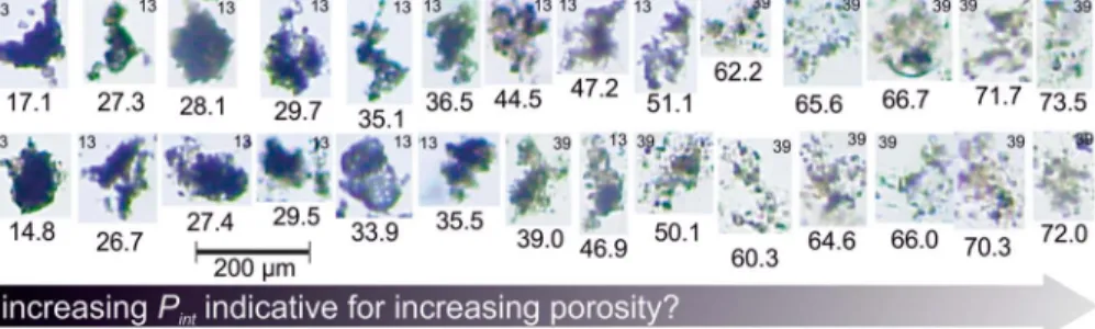
Figure 1.Pint, our proxy for aggregate porosity, can be considered as a size‐normalized measure of particle intensity (equation (3)) where intensity reflects particle transparency. Shown here are randomly taken FlowCam pictures of sinking particles collected in M3 during two sampling days (days 13 and 39 as noted on each picture at the top). The associatedPintvalues (dimensionless) are given below each picture.Pintis higher when the particles are brighter and more transparent, which should be indicative for increased particle porosity (i.e., lower compactness). LowPintparticles on the left side of thefigure were produced under oligotrophic conditions (day 13), while highPintparticles on the right were collected during the massflux event (day 39).
Cmodel¼bbioCreminTz (6) whereCreminis the turnover rate measured in this study andbbiois a scaling factor to achieve a realisticflux attenuation (see below forbbioparameterization). ForTwe used a profile measured near Gran Canaria at the European Station for Time‐Series in the Ocean (29.17°N;−15.50°W; Figure S3) on 26 February 2014 during a cruise with R/VPoseidon(P465). SVmodelincreases with depth according to
SVmodel¼0:04zþSVin−situ (7)
The equations forCmodeland SVmodelwere taken from Schmittner et al. (2008), and their application was justified in Bach et al. (2016). With the averageCremin(0.054 day) and SVin‐situ(37.5 m/day) measured herein (see results) we calculate a mean transfer efficiency from 100 to 1,000 m of 13% with the standardbbio
value of 1.066 used earlier (Bach et al., 2016; Schmittner et al., 2008). Thisflux attenuation is similar to a widely usedMartin bvalue of 0.86 (Martin et al., 1987; please note that we used transfer efficiency 100 to 1,000 m [and not 15 to 1,000 m]) in this case to more easily compare the outcome to those by Martin et al.
(1987). However, attenuation varies seasonally and regionally (Berelson, 2001) and previous studies reported higher or lowerbvalues for the subtropics than 0.86 (Henson, Sanders, et al., 2012; Marsay et al., 2015;
Weber et al., 2016). A comprehensive analysis of regionalizedflux attenuations calculated 897bvalues from underwater camera imaging and 1,971bvalues from POCflux data and found that the medianbvalue in the subtropical NE Atlantic to be ~0.6 (Guidi et al., 2015). Thus, we decreasedbbioin equation (6) from 1.066 to 1.038 to achieve a mean transfer efficiency from 100 to 1,000 m of 25%, which is equivalent to a Martinb value of 0.6 (Guidi et al., 2015; Henson, Sanders, et al., 2012).
The POC massflux to 1,000 m (POC1000) was calculated as POC1000¼POC15
Teff
100 (8)
where POC15is the measured POC massflux at the bottom of the 15‐m deep mesocosms.
3. Results
3.1. Developments in the Plankton Community
The experiment started in oligotrophic conditions with concentrations of all inorganic nutrients close to detection limits (Figure 2). Chl‐a, POC, and BSi concentrations were low during this period and averaged at approximately 0.1μg/L, 9μmol/L, and 0.09μmol/L, respectively (Figure 2). Deep water was added to all mesocosms on day 24, which increased inorganic nutrient concentrations to 3.15, 0.17, and 1.60 mol/L for NOx−, PO43−, and Si (OH)4, respectively. This stimulated a phytoplankton bloom with peak chl‐acon- centrations of 2.61μg/L on day 28. POC increased correspondingly with a slight delay of about 1–2 days (Figure 2). POC concentrations remained at an elevated level after the bloom and decreased only slowly, while chl‐adecreased within a few days after the peak. The decline of BSi after the bloom occurred at a rate ranging between those of chl‐aand POC (Figure 2). TEP concentrations were quite stable and on average 120 μg GXeq L−1before the deep water addition but increased rapidly thereafter right at the point where chl‐a peaked and nutrients were almost exhausted. TEP declined after peak concentrations but remained at ele- vated levels until the end of the experiment. The maximum TEP buildup varied considerably between meso- cosms, ranging from ~300 (M1) to almost 1100 (M9)μg GXeq L−1.
The phytoplankton community was dominated by picophytoplankton and nanophytoplankton during oligo- trophic conditions (days−3 to 24; Figure 3). A bloom ofSynechococcus(0.6–2μm) developed during this phase, which peaked around day 11 (Figure 3b).Synechococcusabundances declined toward the end of Phase I, while picoeukaryotes (0.2–2μm) became more important (Figure 3a). Nanophytoplankton made a stable and significant contribution to chl‐a, while microphytoplankton contributed very little (Figures 3c–3e). The nanophytoplankton contribution remained comparatively stable even after the deep water addition, whereas the relative contribution of picophytoplankton and microphytoplankton reversed.
Microphytoplankton was mostly represented by large chain‐forming diatoms (Leptocylindrus sp., Guinardia sp., and Bacteriastrum sp.) and the prymnesiophyte Phaeocystis sp. (Taucher et al., 2018).
Exceptional to this general pattern were mesocosms M2 and M8 where the toxic phytoplankton species Vicicitus globosus(Dictyochophyceae; Chang et al., 2012) contributed majorly to the deep water‐induced phytoplankton blooms (Riebesell et al., 2018; Figure 3f).
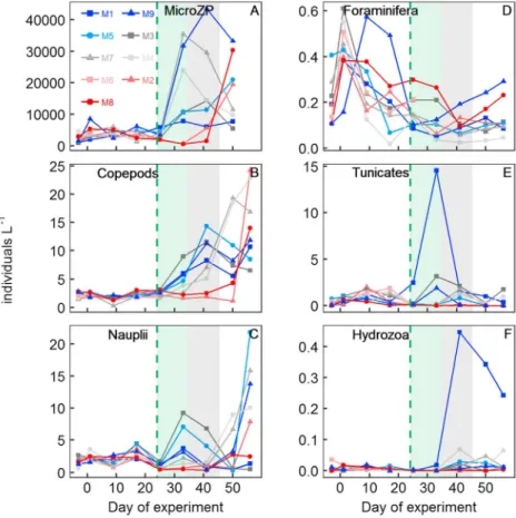
The zooplankton community comprised protists and metazoa. Protists (i.e., microzooplankton, Figure 4a) were mainly represented by aloricate ciliates and small‐sized dinoflagellates (<25μm). Planktonic foramini- fera were an abundant calcifying protist group with all individuals belonging to the family Globigerinidae (Lischka et al., 2018). The most abundant metazoa were copepods, represented primarily by the genera Paracalanus,Clausocalanus,Oithona, andOncaea. Gelatinous zooplankton comprised Hydrozoa with unre- solved taxonomic affiliation and tunicates, represented byOikopleura dioicaandDoliolumsp. A detailed analysis of the zooplankton community can be found in the papers by Lischka et al. (2018), Taucher, Stange, et al. (2018), and Algueró‐Muñiz et al. (2019).
Zooplankton abundances were lower during oligotrophic conditions than after the deep water addition except for foraminifera (Figure 4). Most groups responded to the deep water addition with significant Figure 2.Development of relevant biogeochemical parameters during the experiment. (a) NO3−+ NO2−, (b) PO43−, (c) Si (OH)4, (d) NH4+, (e) chlorophylla, (f) total particulate carbon, (g) biogenic silica, and (h) transparent exopolymer particles. The green dashed line marks the day of the deep water addition. The green‐shaded and the gray‐shaded backgrounds denote the time of the phytoplankton bloom and the diatom massflux event, respectively.
population growth although the response varied profoundly among mesocosms. For example, microzooplankton and copepods (including nauplii) did not respond positively to the deep water addition in M2 and M8 until the bloom of the toxic phytoplanktonV. globosusvanished (compare Figures 3f and 4a–4c). The reason for the large variability of microzooplankton and copepod abundances among the remaining mesocosms is unclear at present. Other important differences were the significant blooms of tunicates (Doliolum sp.) and hydrozoa in M1. Neither of them grew to high abundances in any other mesocosm, although they were present in all of them (Figures 4e and 4f).
3.2. Mass Flux to the Mesocosm Sediment Traps
The massflux of biogenic material (Gcor) can be separated into three phases. Thefirst one comprises the oli- gotrophic conditions and thefirst 10 days after the deep water addition when phytoplankton formed a bloom but the generated biomass was not yet sinking out (days−3 to 34.5). During this initial period, POC, PIC, and BSi massfluxes averaged at 2.93, 0.32, and 0.14 mmol/m2per 48 hr. The second phase lasted for 11 days start- ing 10 days after the deep water addition when the major diatom (orV. globosusin M2 and M8) bloom was sinking out (days 34.5–45.5). POC, PIC, and BSi massfluxes averaged at 29.7, 0.84, and 2.06 mmol/m2per 48 hr during this major sedimentation event. The third phase at the end of the study includes the time after the sedimentation event (days 45.5–55). POC, PIC, and BSi mass fluxes decreased considerably to Figure 3.Phytoplankton groups distinguished by means offlow cytometry. Shown here is the contribution of each group to the total concentration of chlorophyllain the water column. (a) Picoeukaryotes (0.2–2μm), (b) picocyanobacteria (most likelySynechococcusspp.; 0.6–2μm), (c) smaller nanophytoplankton (2–5μm), (d) larger nanophytoplankton (5–8μm), (e) microphytoplankton (≫8μm), and (f) the toxic phytoplanktonVicicitus globosus(~20–30μm). Please note that size range given here accounts for the majority of the gated population but some particles will always be larger or smaller. The plots also show data measured in the Atlantic (black dots) directly next to the mesocosms to illustrate how the enclosure destabilizes the phytoplankton community (section 4.4). The green dashed line marks the day of the deep water addition. The green‐shaded and the gray‐shaded backgrounds denote the time of the phytoplankton bloom and the diatom massflux event, respectively.
time‐integrated averages of 11.34, 0.29, and 0.42 mmol/m2 per 48 hr during the three phases, respectively (Figures 5a–5c).
CaCO3 relative to POC export (i.e., PIC:POC) was initially high (~0.4) but decreased exponentially to reach an average ratio of 0.03 after the deep water addition (Figure 5d). Maximum BSi:POC export ratios were considerably lower than PIC:POC and generally more variable (Figure 5e). BSi:POC averaged at 0.075 from days−3 to 1 and dropped to 0.05 thereafter until day 34. BSi:POC increased during the major sedimentation event (average = 0.067), although with quite a large spread among mesocosms (Figure 5e).
BSi:POC was lowest after the sedimentation event, averaging at 0.04.
3.3. Particle SV, ESD,Pint,Cremin, and RLS
We measured SV, ESD, andPintof 62,481 particles during this study. The SVs of the six designated size classes were 26 ± 7.8 (SV40‐90), 28.2 ± 8 (SV80‐130), 30.8 ± 10 (SV120‐180), 35.6 ± 13.4 (SV170‐260), 43.5 ± 16.8 (SV240‐400), and 62.2 ± 21.4 m/day (SV380‐1000), when averaged over all mesocosms and for the entire experiment. The development of SV over time was slightly different among the different size classes but fol- lowed a similar overarching pattern (Figures 6a–6f). There was a quite pronounced decline in all size classes after thefirst measurement day (day 1). Afterward, SV either remained stable (size classes <130μm) or declined slightly until around day 15. There was a minor peak in SV around day 20 but not in all mesocosms.
SV declined from around day 20 until day 45. The decline in this period was particularly pronounced in some size classes during the major bloom sedimentation event (days 34.5–45.5; e.g. 80–130 µm). SV increased thereafter in all size classes (Figures 6a–6f). The temporal development of SV calculated for the average in situ particle size (SVin‐situ) largely resembled the developments of the largest three size classes (i.e., >170 μm; compare Figures 6d–6f with 7b).
Figure 4.Major zooplankton groups. (a) Microzooplankton, (b) adult copepods and copepodites, (c) nauplii, (d) forami- nifera, (e) tunicates, and (f) hydrozoa. The green dashed line marks the day of the deep water addition. The green‐shaded and the gray‐shaded backgrounds denote the time of the phytoplankton bloom and the diatom massflux event, respectively.
Mean ESDs of particles within the different size classes were 59 ± 6 (40–
90 μm), 101 ± 3 (80–130 μm), 145 ± 4 (120–180 μm), 208 ± 8 (170– 260 μm), 305 ± 14 (240–400μm), and 532 ± 52μm (380–1,000 μm).
The mean values changed only marginally during the experiment (Figures 6g–6l). Thus, changes of mean particle ESD within a size bin can- not explain the pronounced changes in SV of the corresponding size classes. At this point it is important to emphasize that the particle size spectrum determined during the SV measurements is not correctly repre- senting the in situ particle size spectrum. This is because particles used to determine SV have been recovered from the sediment traps through vacuum pumps and have been treated several times before measuring SV in the settling columns (discussed in detail in Bach et al., 2016). To cir- cumvent this problem, we applied a profiling in situ camera system to measure aggregate size spectra in the water column (Taucher, Arístegui, et al., 2018). These measurements revealed that the average size of aggre- gates between 125 and 3,000μm was within a range of 200–260μm for most of the study except for the period of the major sedimentation event where aggregates were larger (Figure 7a). SVin‐situwas affected only to a very small degree by this size increase (Figure 7b).
Mean Pint (dimensionless) increased with size: 17.7 ± 1.5 (40–90 μm), 28.1 ± 4.1 (80–130 μm), 37.3 ± 7 (120–180 μm), 48 ± 10.2 (170–
260 μm), 64 ± 15.7 (240–400 μm), and 99.6 ± 25 (380–1,000 μm).
Accordingly,Pintreproduces the expected increase of porosity with size (Burd & Jackson, 2009; Logan & Wilkinson, 1990) due to the depen- dency ofPinton ESD (see equation (3)).Pintwas increasing in most size classes until the major bloom sedimentation event (Figures 6m–6r). The increase was larger in the smaller size classes, and hardly any change was observed in the two largest size classes. Pint increased rapidly at the onset of the sedimentation event. Conversely to the trends prior to this event, the increases were more pronounced in the larger size classes. In this case, no increase was observed in the smallest size class.
Pint decreased to a variable degree in all size classes after the bloom sedimentation (Figures 6m–6r). SVs of all size classes were negatively correlated withPint(Figure 9a).
POC remineralization (Cremin) was determined on nine occasions during the mesocosm experiment (Figure 7c). Unfortunately, technical problems with the equipment prevented us from doing incubations before day 11.
The estimatedCreminuncertainty of 35% (section 2.4) and the lower tem- poral resolution of this data set complicated the detection of trends over time since only very clear changes can be distinguished from noise (Figure 7c). On average,Creminwas higher during thefirst incubation with the highest value in M9 (0.125 day), while the lowestCreminwas observed in M8 during the phytoplankton bloom (0.007 day). High values were also measured during the major sedimentation event (days 37 and 41), although only in M3, M5, and M7.Cremindeclined in almost all meso- cosms after the sedimentation event (Figure 7c).
RLS ranged between 0.0002 and 0.004 m−1, and the temporal develop- ment largely resembled the development ofCremin(compare Figures 7c and 7d). The influence of Cremin on RLS was dominant because its changes during the study were approximately fifteenfold, while the changes in SVin‐situwere approximately threefold (compare Figures 7b and 7c). Nevertheless, SVin‐situhad a noticeable influence on RLS due to Figure 5.Massflux of sinking organic material and ballast minerals into the
sediment trap. (a) POC, (b) PIC, (c) BSi, (d) PIC:POC, and (e) BSi:POC.
The green dashed line marks the day of the deep water addition. The green‐shaded and the gray‐shaded backgrounds denote the time of the phytoplankton bloom and the diatom massflux event, respectively.
the generally decreasing trend from initially ~50 to ~30 m/day at the end of the study. This decrease was reflected in particularly high RLS during the major sedimentation event.
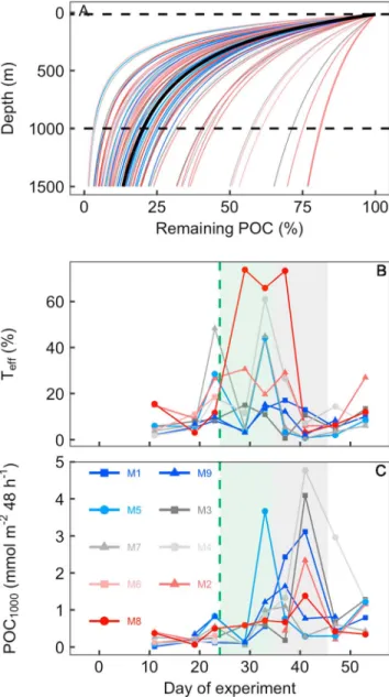
3.4. Estimated Transfer Efficiency and Mass Flux to the Deep Ocean
The degree offlux attenuation varied widely over the course of the study, largely driven by thefluctuations in Cremin. Accordingly, the temporal pattern ofTefflargely resembled the inverse ofCremin(compare Figures 7c and 8b).Teffranged from 0.6% to 74% with the majority of values between 0.6% to 20%. POC1000ranged between 0.01 and 4.8 mmol/m2per 48 hr and was generally higher during the massflux event than during oligotrophic conditions (Figure 8c).
4. Discussion
4.1. Pint—A Useful Optical Proxy for Aggregate Porosity?
Porosity indicates the fraction of an aggregate not occupied by solid matter (Alldredge & Gotschalk, 1988). A porous aggregate will usually have a lower density and therefore sink slower than a more compact one, given that both have the same size, shape, and are made of solid matter of a similar density. Thus, porosity is an important variable affecting aggregate SV and ultimately POC export (Burd & Jackson, 2009).
Figure 6.Temporal development of sinking velocity (SV), ESD, and the porosity proxyPint. (a–f) SV of the different particle size classes, (g–l) mean ESD, and (m–r)Pintof the corresponding size classes. Please note that the size classes are reported at the top of each subplot. The black line on each plot is the daily average of all mesocosms and is shown to facilitate the detection of general trends. The green dashed line marks the day of the deep water addition. The green‐ shaded and the gray‐shaded backgrounds denote the time of the phytoplankton bloom and the diatom massflux event, respectively.
Porosity can be measured directly by embedding aggregates in resins or gels and thin slicing them to determine their structure microscopically (Chu et al., 2004; Flintrop et al., 2018; Leppard et al., 1996). These mea- surements provide an unprecedented level of detail of the aggregate matrix but are too time‐consuming and expensive to apply to the thou- sands of aggregates investigated here. Alternatively, porosity can be calcu- lated from dry weight measurements or density estimations, but these calculations are associated with numerous assumptions and must be regarded with care (Alldredge & Gotschalk, 1988; Engel et al., 2009;
Logan & Wilkinson, 1990; Helle Ploug et al., 2008). Here we derivesize‐
normalized particle intensity(Pint) as an independent and easily measur- able proxy for porosity. The underlying assumption is that aggregates within a narrow size range appear brighter when they are more porous because more of the light passes through the back‐light‐illuminated aggregate (section 2.6).
The best way to assess the valuePintwould be a comparison to an indepen- dent porosity approximation. In similar data set from the Norwegian coast, we estimated porosity from calculated aggregate excess densities and solid matter density of sediment trap material using Stokes' law (Bach et al., 2016). Unfortunately, Stokes' law was not applicable in the present experiment because SV (and therefore Reynolds numbers) were too high so that most particles did not sink in a laminar flow regime (McNown & Malaika, 1950). Thus, at this stage we can only argue that Pint is a useful proxy without independent validation. Perhaps the strongest support for its usefulness comes from the pictures shown in Figure 1. These were taken randomly from measurements in M3 and show that aggregates with higherPintvalues on the right side of Figure 1 do indeed appear to be more porous. The porous aggregates were filmed mostly during the massflux event where concentrations of TEP were con- siderably higher (Figure 2h). TEP serves as glue within the aggregate matrix, and high concentrations should increase the probability tofind loosely attached phytoaggregates, which have not experienced much (re) packaging (Burd & Jackson, 2009). However,Pintcould also be affected by the chemical composition of the aggregate matrix, which, like porosity, influences the intensity (i.e., thebrightness) of a particle. For example, interstitial space in aggregates could befilled with CaCO3or TEP, and this would in both cases reduce the porosity. However, CaCO3absorbs more light than TEP and therefore affectsPintdifferently. The problem of mate- rial transparency could be circumvented to some extent by staining trans- parent components within the aggregate matrix (Cisternas‐Novoa et al., 2015), but this has not been done here. Thus, the unknown chemical composure of aggregates must be considered as confounding factor for the porosity approximation withPint.
The temporal development of Pintreveals distinct features that further strengthen our confidence in this proxy. For example, there was a sudden increase ofPintat the onset of the massflux event (see Figures 6m–6r, par- ticularly the larger size classes). We observed exactly the same kind of sudden increase during the onset of mass flux event in a mesocosm study at the Norwegian coast where porosity was assessed differently (Bach et al., 2016). Thus, the similarity in the response patterns with two independent porosity approxima- tions supports both of them.
Furthermore, the mesocosm‐specific development ofPintduring the massflux event provides additional support. The major bloom formers after the deep water addition were diatoms, but these were less Figure 7.Size, SVin-situ, and remineralization of sinking material.
(a) Average size of particles >125μm inside the mesocosms as determined with an in situ camera system. (b) SVin‐situcalculated with daily ESD versus SV relationships measured with the FlowCam using in situ particle size as input data. (c) C‐specific remineralization rate (Cremin).
(d) Remineralization length scale. The green dashed line marks the day of the deep water addition. The green‐shaded and the gray‐shaded backgrounds denote the time of the phytoplankton bloom and the diatom massflux event, respectively.
increases due to the formation of highly porous diatom aggregates, com- bined with the lack of microzooplankton and mesozooplankton grazers during this period (check Figure 4 for zooplankton). This adds addi- tional confidence to the value ofPintas porosity proxy.
Vertical particle profiles determined with in situ camera systems are becoming an increasingly important tool to estimate carbon exportfluxes (Boss et al., 2015; Guidi et al., 2008; Iversen et al., 2010). Camera‐based massflux calculations utilize particle abundance data and a theoretical size versus SV relationship (Guidi et al., 2008). However, Figure 6 illustrates that size alone is insufficient to predict SV as it changes approximately threefold in the course of the study, while aggregate sizes remain largely constant.
The utilization of thePintversus SV relationships shown in Figure 9a may therefore help to improve the determination of massflux, at least with back‐light‐illuminated camera systems wherePintcould be determined.
4.2. Influence of Ballast Minerals and Plankton Community Structure on SV
The development of SV over time reveals distinct patterns that can be linked to processes in the plankton community. SV was relatively high during thefirst 2 weeks of the experiment, particularly in the size classes
>170μm (Figures 6a–6f). One likely reason for this was the initially high ballasting with CaCO3(Figure 5d), but the question is what generated this ballast? The two calcifying groups that were found in relevant quantities were coccolithophores and foraminifera (Lischka et al., 2018; W. Guan, personal communication). Coccolithophores were present only until the deep water addition in abundancesfluctuating between below detection limit and 1.5 cells per milliliter (W. Guan, personal communication). If we assume a per cell PIC content of a heavily calcified species (25 pmol per cell forCoccolithus pelagicus; Bach et al., 2015), we would in the high- est possible case (1.5 cells per milliliter) reach a coccolithophore PIC of 0.04 μmol/L. Hence, if such an amount sank out in 48 hr (i.e., 0.43 mmol/m2per 48 hr), it could explain the initial PICflux to the sediment traps (Figure 5b). However, since the 0.04 mmol/L is an upper bound, we consider coccolithophores to contribute generally much less CaCO3
ballast. Foraminifera were represented by very small (50–200 μm) Globigerinidae species (Lischka et al., 2018). The highest measured sedi- mentationflux was 0.14 individual per liter per 48 hr (~1,500 individuals per square meter per 48 hr) but generally well below this value (Lischka et al., 2018). Based on published size to weight relationship for the two Globigerinidae species (Lombard et al., 2010), we estimate that a 200‐μm individual would have contained less than 10‐μg CaCO3 (~0.1‐μmol PIC). Thus, the PICflux by foraminifera tests could maximally have been 0.15 mmol/m2per 48 hr, but likely much lower most of the time. Furthermore, foraminifera shells do not integrate particularly well into aggregate matrices so that their accelerating effect on SV should be minor (Schmidt et al., 2014).
Figure 8.Transfer efficiency (Teff) and massflux to the deep ocean based on SVin‐situandCreminusing model equations (4) and (5). (a) Calculatedflux attenuation profiles of organic material collected in the mesocosm sediment traps while sinking to depth. Each of the 73 thin lines represents one attenuation profile as calculated with equation (5) using one of the 73 measuredCreminvalues and the 73 corresponding SVin‐situvalues, respec- tively (Creminvalues from Figure 7c and corresponding SVin‐situfrom Figure 7b). The color code corresponds to the mesocosms where the SVin‐situandCremincombination was measured. The thick black line is the attenuation profile calculated with the average of all 73Creminvalues (i.e., 0.054 day) and the average of the corresponding 73 SVin‐situvalues (37.5 m/day). The horizontal dashed black lines mark the 15‐(bottom of mesocosm) and 1,000‐m depths, respectively. (b)Teffbetween 15 and 1,000 m derived from calculations with equation (5). These are the intercepts where the individual profiles from plot (a) cross the 1,000‐m depth level.
(c) Massflux at 1,000‐m depth as calculated with equation (8). The green‐ shaded and the gray‐shaded backgrounds in (b) and (c) denote the time of the phytoplankton bloom and the diatom massflux event, respectively.
Based on the above mentioned assessments, it seems unlikely that bio- genic CaCO3is fully accountable for the PIC massflux observed in the mesocosm sediment traps. Lithogenic carbonates could enter the meso- cosms at the surface via airborne dust influx, which regularly occurs in the Canary Island region (Gelado‐Caballero et al., 2012; Neuer et al., 2004; Nowald et al., 2015), although dust dry deposition was not particu- larly high during thefirst week of the study when PIC:POC was highest (D. Gelado‐Caballero, personal communication). Alternatively, resus- pended carbonate sediments enclosed initially may have started to sink out as soon as the mesocosms were closed and the turbulence declined.
The exponentially decreasing PIC:POC ratio in the sediment traps lends some support for this hypothesis (Figure 5d).
The plankton size structure was likely another important reason for gen- erally higher SV during thefirst half of the study.Pint, our proxy for por- osity, was generally lower during thefirst 2 weeks indicating that the plankton community produced relatively compact detritus when oligo- trophic conditions prevailed (Figures 1 and 6m–6r). Oligotrophy is usually characterized by the dominance of picophytoplankton and small nano- phytoplankton (Chisholm, 1992), which provide small aggregate building blocks allowing little interstitial space between them when they aggregate (Burd & Jackson, 2009). Furthermore, organic biomass is considered to be recirculated more intensely through the food web under stable oligo- trophic conditions thereby generating higher aggregate compactness than in more unstable environments (Fischer & Karakaş, 2009; Francois et al., 2002; Lam et al., 2011). However, we consider this second mechanism not to be relevant in our study because the enclosure of the phytoplankton communities destabilized the oligotrophic food web as will be argued in section 4.5.
The deep water addition on day 24 initiated a phytoplankton bloom, which quickly ran into nitrogen limitation and peaked around day 29 (Figures 2a, 2e, and 2g; Taucher, Stange, et al., 2018). TEP concentrations increased sharply after the chl‐apeak and promoted the initiation of an aggregation event that lasted for 10 days until aggregates reached their maximum size and sank down during the massflux event between days 35 and 48 (Figures 2h and 5a; Stange et al., 2017; Taucher, Arístegui, et al., 2018). The diatom bloom and the simultaneous formation of increasingly large aggregates coincided with a considerable reduction of SV, even though opal ballast increased during the massflux event (Figures 6a–6f and 5e). Thus, the accelerating influence of opal ballast on aggregate excess density must have been overcompensated by reduced compactness.
There are four lines of evidence supporting this conclusion. First, nutrient injections into the prevailing oligotrophic conditions shifted the phyto- plankton size structure toward larger species (Figure 3). Larger species should form more porous aggregates because (i) they provide more interstitial space within the aggregate matrix and (ii) they are transiently relieved from biotic repackaging because they outgrew copepod grazers (compare Figures 2e and 4b). Indeed,Pintincreases substantially dur- ing the massflux event which is not only very clear in the data (Figures 6m–6r but with the exception of 40–90μm) but also obvious when comparing pictures of aggregates from the massflux event with those photographed during the oligotrophic phase (Figure 1). Second, relatively high concentrations of TEP after the bloom (Figure 2h) may have decelerated sinking because TEP is positively buoyant and, due to its sticki- ness, causes a more porous aggregate structure, which further reduces their excess density (Azetsu‐Scott &
Passow, 2004; Engel & Schartau, 1999; Mari, 2008; Mari et al., 2017). Third, we have made the identical observation during diatom blooms in the mesocosm study in Norway and came to the same porosity‐based Figure 9.Correlations between SV,Pint, and the ratio of picophytoplankton
to nanophytoplankton and microphytoplankton (P/NM). The different colors from warm to cold represent the six different particle size classes:
orange = 40–90μm, yellow = 80–130μm, turquoise = 120–180μm, blue‐ green = 170–260μm, blue = 240–400μm, and dark blue = 380–1,000μm (see also the legend in the top panel). All correlations shown here are significant (p≪0.01). (a) SV is negatively correlated withPintin all size classes;R240‐90= 0.09,R280‐130= 0.12,R2120‐180= 0.21,R2170‐260= 0.38, R2240‐400= 0.34,R2380‐1000= 0.27. (b) SV is positively correlated with P/NM in all size classes;R240‐90= 0.14,R280‐130= 0.04,R2120‐180= 0.14, R2170‐260= 0.27,R2240‐400= 0.31,R2380‐1000= 0.15. (c)Pintis negatively correlated with P/NM in all size classes;R240‐90= 0.18,R280‐130= 0.47, R2120‐180= 0.49,R2170‐260= 0.41,R2240‐400= 0.30,R2380‐1000= 0.14.
Please note that thexaxis scaling in b and c is log10 transformed and the numbers on the axis show the exponent (e.g.,−1 = 10−1= 0.1 chla:chla).
Regression equations are provided in Table S1.