Veröffentlichungen der DGK
Ausschuss Geodäsie der Bayerischen Akademie der Wissenschaften
Reihe C Dissertationen Heft Nr. 840
Mahmud Haghshenas Haghighi
Local and Large Scale InSAR Measurement of Ground Surface Deformation
München 2019
Verlag der Bayerischen Akademie der Wissenschaften
ISSN 0065-5325 ISBN 978-3-7696-5252-9
Diese Arbeit ist gleichzeitig veröffentlicht in:
Wissenschaftliche Arbeiten der Fachrichtung Geodäsie und Geoinformatik der Universität Hannover ISSN 0174-1454, Nr. 354, Hannover 2019
Veröffentlichungen der DGK
Ausschuss Geodäsie der Bayerischen Akademie der Wissenschaften
Reihe C Dissertationen Heft Nr. 840
Local and Large Scale InSAR Measurement of Ground Surface Deformation
Von der Fakultät für Bauingenieurwesen und Geodäsie der Gottfried Wilhelm Leibniz Universität Hannover
zur Erlangung des Grades Doktor-Ingenieur (Dr.-Ing.) genehmigte Dissertation
Vorgelegt von
M.Sc. Mahmud Haghshenas Haghighi
Geboren am 03.03.1986 in Estahban
München 2019
Verlag der Bayerischen Akademie der Wissenschaften
ISSN 0065-5325 ISBN 978-3-7696-5252-9
Diese Arbeit ist gleichzeitig veröffentlicht in:
Wissenschaftliche Arbeiten der Fachrichtung Geodäsie und Geoinformatik der Universität Hannover ISSN 0174-1454, Nr. 354, Hannover 2019
Adresse der DGK:
Ausschuss Geodäsie der Bayerischen Akademie der Wissenschaften (DGK) Alfons-Goppel-Straße 11 ● D – 80539 München
Telefon +49 – 331 – 288 1685 ● Telefax +49 – 331 – 288 1759 E-Mail post@dgk.badw.de ● http://www.dgk.badw.de
Prüfungskommission:
Vorsitzender: Prof. Dr.-Ing. Christian Heipke Referent: Prof. Dr. Mahdi Motagh
Korreferenten: Prof. Falk Amelung (University of Miami) Prof. Dr.-Ing. Steffen Schön
Tag der mündlichen Prüfung: 27.06.2019
© 2019 Bayerische Akademie der Wissenschaften, München
Alle Rechte vorbehalten. Ohne Genehmigung der Herausgeber ist es auch nicht gestattet,
die Veröffentlichung oder Teile daraus auf photomechanischem Wege (Photokopie, Mikrokopie) zu vervielfältigen
ISSN 0065-5325 ISBN 978-3-7696-5252-9
3
Abstract
Interferometric Synthetic Aperture Radar (InSAR) is a remote sensing technique frequently used for measuring Earth’s surface deformation. InSAR time series approaches provide detailed information about the evolution of displacement in time and also overcome the limitations of conventional InSAR.
Both InSAR and InSAR time series methods have been used for measuring tectonic and non-tectonic surface deformations caused by natural and anthropogenic processes in local to regional scales. In the past, the availability of SAR data suitable for InSAR purpose was a major constraint for InSAR applications in many areas of the world. The launch of the Sentinel-1 mission in 2014 guaranteed a regular long-term acquisition plan of SAR data available all over the globe that enables us to increase the scale of deformation mapping from regional to national. However, there are challenges in large- scale InSAR processing that needs to be addressed. In this thesis, InSAR time series approaches are used to obtain detailed maps of the time-varying surface displacement fields caused by non-tectonic processes at a local to regional scales and find the link between surface displacement and its drivers.
Then, a workflow for large-scale InSAR time series analysis is suggested that benefits from extensive collections of data provided by Sentinel-1 to identify and monitor displacement fields over extensive areas.
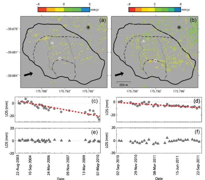
In the first part of this thesis, InSAR time series approaches are used at local to regional scales in three independent case studies. In the first case study, a localized displacement of as much as 1 cm/yr attributed to slope movement of a landslide in Taihape, New Zealand is observed. Along with the long- term trend of displacement caused by slope movement, the analysis of time series reveals an acceleration in surface displacement due to a rainstorm as well as the seasonal variations of displacement linked to groundwater variations. In the second study area, land subsidence in Tehran, Iran is analyzed at a regional scale. Using an extensive collection of SAR data, land subsidence areas with a peak exceeding 25 cm/yr are detected. After combining time series from different datasets, both long-term subsidence trend due to the constant decline of groundwater level, and seasonal variations of surface displacement linked to the discharge/recharge cycle of groundwater are investigated. In the third case study, localized displacement of a natural gas reservoir in Berlin is analyzed and a long-term uplift of approximately 0.2 cm/yr and 2 cm of seasonal variations linked to the injection of gas in summer and extraction in winter are observed. Furthermore, mining-induced displacements in an area near Leipzig are measured and approximately 4 cm/yr of subsidence coupled with 5 cm/yr of east-west displacement are observed.
To extend the InSAR measurement of non-tectonic displacement fields from local and regional to national scale, a workflow is developed in this thesis that benefits from the vast amount of data col-
4
lected by Sentinel-1 mission. The proposed workflow notably reduces the broad-scale and topography- dependent components of tropospheric errors in an adaptive approach and provides a quick, but robust displacement field map from large stacks of Sentinel-1 data. The proposed method is applied on two tracks of Sentinel-1 data across Iran and Germany and successfully obtained the displacement fields in large scales. In the first case study, more than 20 displacement areas mostly attributed to land subsidence induced by over-extraction of groundwater are identified. In the second case study, approx- imately 10 displacement areas mainly related to anthropogenic activities including mining and gas/oil injection/extraction are detected.
Keywords: InSAR, Displacement time series, large-scale mapping, Land subsidence, Landslide, anthropogenic deformation
5
Zusammenfassung
Radarinterferometrie (InSAR) ist eine Fernerkundungsmethode, die häufig zur Messung von Erdober- flächenverformungen eingesetzt wird. InSAR-Zeitreihen-Ansätze liefern detaillierte Informationen über die Entwicklung der Verformung in der Zeit und überwinden zudem die Grenzen des konventionellen InSAR. Sowohl InSAR als auch InSAR-Zeitreihenmethoden wurden auf lokaler bis regionaler Ebene zur Messung tektonischer und nicht-tektonischer Oberflächenverformungen infolge natürlicher und anthropogener Prozesse eingesetzt. In der Vergangenheit war die Verfügbarkeit von SAR-Daten, die für InSAR-Zwecke geeignet sind, für viele Gebiete in der Welt ein wesentliches Hindernis für InSAR-Anwendungen. Der Start der Mission Sentinel-1 im Jahr 2014 garantierte einen regelmäßigen, langfristigen Akquisitionsplan für SAR-Daten sowie eine weltweiten Verfügbarkeit und ermöglicht es damit den Umfang der Deformationskartierung von regional auf national zu erhöhen. Es gibt je- doch Herausforderungen bei der groß angelegten InSAR-Verarbeitung, die es zu bewältigen gilt. In dieser Arbeit werden InSAR-Zeitreihenansätze verwendet, um detaillierte Karten der zeitvariablen Oberflächenverformungsfelder nicht-tektonischer Prozesse auf lokaler bis regionaler Ebene zu erhalten, welche dazu dienen den Zusammenhang zwischen Oberflächenverlagerungen und ihren Ursachen zu finden. Anschließend wird ein Workflow für die groß angelegte InSAR-Zeitreihenanalyse vorgeschlagen, der von den umfangreichen Datensammlungen von Sentinel-1 zur Identifizierung und Überwachung von Deformationsfeldern über große Gebiete hinweg profitiert.
Im ersten Teil dieser Arbeit werden InSAR-Zeitreihenansätze auf lokaler bis regionaler Ebene in drei unabhängigen Fallstudien verwendet. In der ersten Fallstudie wird eine lokale Verschiebung von bis zu 1 cm/a beobachtet, die auf die Hangbewegung eines Erdrutsches in Taihape, Neuseeland, zurück- zuführen ist. Neben dem langfristigen Trend der Verschiebung durch die Hangbewegungen zeigt die Analyse von Zeitreihen eine Beschleunigung der Oberflächenverschiebung durch einen Regensturm sowie saisonale Verschiebungen durch Grundwasserschwankungen. Im zweiten Untersuchungsgebiet, der Landabsenkung in Teheran, wird der Iran auf regionaler Ebene analysiert. Mit einer umfangre- ichen Sammlung von SAR-Daten werden Landabsenkungsgebiete mit einer Höchstrate von mehr als 25 cm/a detektiert. Mit Hilfe einer Kombination von Zeitreihen aus verschiedenen Datensätzen werden sowohl der langfristige Absenkungstrend aufgrund des konstanten Absinkens des Grundwasserspiegels als auch saisonale Schwankungen der Oberflächendeformation im Zusammenhang mit dem Abfluss- /Zuflusszyklus des Grundwassers untersucht. In der dritten Fallstudie wird die lokale Deformation eines Erdgasspeichers in Berlin analysiert und eine langfristige Hebung von ca. 0,2 cm/a und 2 cm saisonale Schwankungen im Zusammenhang mit der Gaseinleitung im Sommer und der Förderung im Winter beobachtet. Darüber hinaus werden bergbaubedingte Verlagerungen in einem Gebiet bei Leipzig gemessen und ca. 4 cm/a Absenkung bei gleichzeitiger 5 cm/a Ost-West-Verschiebung
6
beobachtet. Um die InSAR-Messung von nicht-tektonischen Deformationsfeldern von der lokalen und regionalen auf die nationale Ebene zu erweitern, wird in dieser Arbeit ein Workflow entwickelt, der von der großen Menge aufgenommener Sentinel-1-Missionsdaten profitiert. Der vorgeschlagene Workflow reduziert insbesondere die großräumigen und topographieabhängigen Komponenten troposphärischer Fehler in einem adaptiven Ansatz und liefert eine schnelle, aber robuste Oberflächenverformungskarte aus großen Stapeln von Sentinel-1-Daten. Die vorgeschlagene Methode wird auf zwei Tracks von Sentinel-1-Daten im Iran und in Deutschland angewendet und ermittelt erfolgreich die großräumigen Deformationsfelder. In der ersten Fallstudie werden mehr als 20 Verformungsgebiete identifiziert, die meist auf Bodensenkungen, verursacht durch Überbeanspruchung des Grundwassers, zurückzuführen sind. In der zweiten Fallstudie werden etwa 10 Deformationsgebiete erfasst, die hauptsächlich mit anthropogenen Aktivitäten wie Bergbau und Gas/Erdöl Einspeisung/Extraktion zusammenhängen.
Contents 7
Contents
1. Introduction 11
1.1. Research Objectives . . . 13
1.2. Outline and Structure of the Thesis . . . 14
2. Theoretical Background 17 2.1. Introduction . . . 18
2.2. SAR Imaging . . . 18
2.2.1. SAR Image Distortions . . . 19
2.2.2. SAR Imaging Modes . . . 20
2.2.3. SAR Missions . . . 20
2.3. SAR Interferometry . . . 21
2.3.1. InSAR Workflow . . . 21
2.3.2. InSAR Decorrelation . . . 24
2.3.3. Errors in InSAR . . . 25
2.3.4. Examples of Interferograms . . . 28
2.3.5. Decomposition of Line-of-Sight Measurements . . . 29
2.4. Multi Temporal InSAR . . . 29
2.4.1. Scattering Mechanisms in SAR Images . . . 30
2.4.2. Interferogram Stacking . . . 30
2.4.3. Persistent Scatterer InSAR . . . 31
2.4.4. Small Baseline InSAR . . . 32
2.5. Analysis of Displacement Time Series . . . 33
2.5.1. Continuous Wavelet Transform . . . 34
2.5.2. Cross Wavelet Transform . . . 34
2.5.3. Application of CWT and XWT to InSAR Time Series . . . 35
3. Methodological Contribution 37 3.1. Introduction . . . 38
3.2. Challenges in Large-scale InSAR . . . 38
3.3. Proposed Method . . . 39
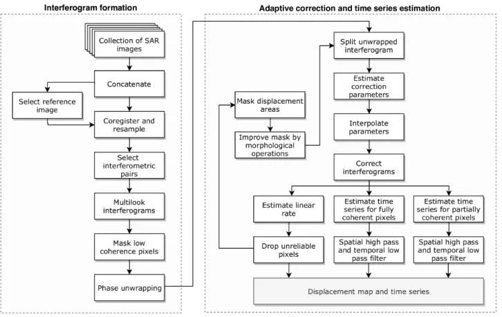
3.3.1. Interferogram Formation . . . 39
3.3.2. Adaptive Correction of Interferograms . . . 41
3.3.3. Estimating the Displacement Rate . . . 42
3.3.4. Estimating the Time Series of Displacement . . . 42
8 Contents
4. InSAR Monitoring of Localized Landslide in Taihape, New Zealand 43
4.1. Abstract . . . 44
4.2. Introduction . . . 44
4.3. Study Area . . . 45
4.4. Methods . . . 46
4.4.1. InSAR Measurement . . . 46
4.4.2. Ancillary Data . . . 47
4.4.3. Cause-Effect Analysis . . . 48
4.5. Results . . . 48
4.5.1. Small-baseline Interferograms . . . 48
4.5.2. Time-series Results . . . 49
4.6. Discussion . . . 50
4.6.1. Suitability of InSAR Measurements for Monitoring the Taihape Landslide . . . 50
4.6.2. Interpretation of InSAR Results . . . 52
4.6.3. Comparison with Ground Truth . . . 52
4.6.4. Comparison with Rainfall and Groundwater Level . . . 53
4.7. Conclusion . . . 56
4.8. Acknowledgments . . . 57
4.9. Supplementary Materials . . . 58
5. InSAR Measurement of Regional Land Subsidence in Tehran, Iran 61 5.1. Abstract . . . 62
5.2. Introduction . . . 62
5.3. Study Area and Problem Description . . . 63
5.4. Datasets . . . 66
5.4.1. SAR Data . . . 66
5.4.2. Leveling . . . 67
5.4.3. Groundwater Level . . . 67
5.5. Methods . . . 67
5.5.1. Multi-temporal InSAR Analysis . . . 67
5.5.2. Merging InSAR Time Series . . . 71
5.5.3. Cause-Effect Analysis . . . 72
5.6. Results . . . 73
5.6.1. Southwest of Tehran . . . 73
5.6.2. IKA Airport . . . 75
5.6.3. Varamin County . . . 76
5.6.4. Time Series of Displacement . . . 77
5.6.5. Accuracy, Precision and Consistency Assessments . . . 78
5.7. Discussion . . . 81
5.7.1. Structural Control of the Displacement . . . 81
5.7.2. Comparison with Groundwater . . . 82
5.7.3. Elastic vs. Inelastic Compaction . . . 85
Contents 9
5.8. Conclusion . . . 86
5.9. Acknowledgments . . . 87
5.10. Supplementary materials . . . 87
5.10.1. Significance of Tropospheric Delay . . . 87
5.10.2. Decomposition of LOS Measurement . . . 88
5.10.3. Under/Overestimation of Displacement Rates . . . 89
6. Sentinel-1 InSAR Measurement of Anthropogenic Deformation in Germany 91 6.1. Summary . . . 92
6.2. Introduction . . . 92
6.3. Sentinel-1 InSAR Processing . . . 94
6.4. Large-scale Sentinel-1 Processing . . . 98
6.5. Anthropogenic Ground Motion in Berlin . . . 100
6.6. Mining-induced Deformation in Leipzig . . . 104
6.7. Conclusions and Prospect . . . 107
6.8. Acknowledgements . . . 108
7. Subsequent Work: Measurement of Localized Deformations over Extensive Areas 109 7.1. Introduction . . . 110
7.2. SAR Datasets . . . 110
7.3. Sentinel-1 Interferograms . . . 110
7.4. Corrected Interferograms . . . 112
7.5. Displacement Maps and Time Series . . . 114
7.6. Discussion . . . 118
7.7. Conclusion . . . 121
8. Cooperation Works 123 8.1. Quantifying Land Subsidence in the Rafsanjan Plain, Iran Using InSAR Measurements 124 8.1.1. Abstract . . . 124
8.1.2. Author Contribution . . . 124
8.2. Characterizing Post-construction Settlement of Masjed-Soleyman Dam Using TerraSAR-X SpotLight InSAR . . . 125
8.2.1. Abstract . . . 125
8.2.2. Author Contribution . . . 126
8.3. InSAR Observation of the 18 August 2014 Mormori (Iran) Earthquake . . . 126
8.3.1. Author Contribution . . . 126
9. Summary and Future Work 129 9.1. Future works . . . 132
A. Software and Tools 135
Bibliography 137
Chapter 1
Introduction
12 1. Introduction
Geohazards, natural or anthropogenic, substantially influence the life of many people across the globe. They can be catastrophically rapid, like earthquakes or volcanic eruptions, or slowly degrad- ing the living environment like land subsidence or slow-moving landslides. Geohazards are enormous threats to human life, civilian properties, and infrastructure. For example, from 2004 to 2016, ap- proximately 4700 distinct non-seismic landslides were detected to be responsible for a total of 56000 fatalities across the globe. Such landslides are widespread globally and their anthropogenic occurrence is growing in recent years (Froude and Petley, 2018). As another example, land subsidence associated with excessive groundwater pumping is an increasing challenge in many areas. Groundwater is the primary source of freshwater in semi-arid to arid regions of the world. Unsustainable depletion of groundwater is an immense problem endangering the availability of water to approximately 1.7 billion people (Gleeson et al., 2012) and posing a significant hazard due to associated land subsidence.
We need to enhance our understanding of geohazards and develop solutions to reduce their inherent risks. In this regard, detailed geodetic measurements are critical for the detection, study and under- standing of earth surface processes and geohazards, yet their field measurements are time-consuming and expensive. In this regard, Interferometric Synthetic Aperture Radar (InSAR) has been widely used in the past three decades as a powerful geodetic method that provides valuable insight into spatial and temporal kinematics of earth processes from space (Rosen et al., 2000; Bürgmann et al., 2000). The main advantage of InSAR is its ability to provide precise displacement measurements over large areas. Decorrelation of interferometric phase, due to temporal variations of earth surface or imaging geometries, is one of the main limitations of InSAR (Zebker and Villasenor, 1992). Moreover, remaining errors, particularly from atmospheric phase delay, may reach several centimeters across the interferogram and obscure the desired signal (Hanssen, 2001).
With the increasing availability of multi-temporal SAR data in the past decades, different time series approaches have been developed to address the limitations of conventional InSAR. They can be classified into two main branches, Persistent Scatterer InSAR (PS) (Ferretti et al., 2001; Hooper et al., 2004) and Small Baseline (SB) (Berardino et al., 2002; Hooper, 2008). Both mentioned approaches search for coherent pixels in a stack of SAR data and connect their interferometric phase in time to obtain the displacement history of each pixel. Furthermore, they either use external information or implement temporal and spatial filters to reduce the errors and extract the displacement signal properly (Hooper et al., 2012).
Several SAR sensors have been launched in the past three decades for both commercial and scientific purposes. As a result, in many areas of the world, a rich collection of SAR data is available that can be used for the historical analysis of displacement. The launch of the Sentinel-1 mission in 2014 has dramatically increased the availability of SAR data. Regular SAR data acquisition by Sentinel-1 gives a unique opportunity for displacement monitoring anywhere in the world (Torres et al., 2012; Salvi et al., 2012). However, new methods are needed to efficiently deal with the massive amount of acquired data and extract relevant information from them.
1.1. Research Objectives 13
1.1. Research Objectives
This thesis deals with InSAR geodetic measurements for a better understanding of geohazards at local to regional scales from two major aspects. The first aspect is monitoring, which is the precise measurement of the earth’s surface deformation at specific locations in order to understand the past behavior and current status of the processes. The second aspect is detection, which is the large-scale surveys of local to regional deformations to identify specific geohazard hot spots for further precise measurement and monitoring.
The first major aspect, measurement and monitoring of local to regional geohazards, is performed for four different areas prone to different geohazards caused by slope instability, groundwater extraction, open-pit mining, and underground gas injection/extraction. InSAR time series analysis approaches are utilized to obtain the history of displacement from older SAR data and the current status from the recent SAR data. Then, the results of InSAR time series are used to find the link between the surface displacements and their driving mechanisms.
The second major aspect of this thesis is to assess the potentials of the Sentinel-1 mission in large- scale detection of local to regioanl geohazards. In this regards, this thesis suggests a novel method that benefits from massive and regular data acquisition of Sentinel-1 mission for detection of local to regional displacements in a broad area. This approach reduces the tropospheric phase delay, which is a significant error source in large-scale InSAR, and robustly estimates the displacement time series.
This thesis discusses several challenges of InSAR time series analysis and the approaches to tackle them. One of the main challenges is the effect of tropospheric phase delay. The performance of InSAR time series analysis in reducing the tropospheric artifact in local to regional scales are assessed in this thesis. Furthermore, the effectiveness of external atmospheric models in correcting InSAR measurements is investigated. Another challenges of InSAR time series analysis, in particular with older SAR sensors, is their irregular and sporadic data acquisitions. New generations of SAR sensors, particularly Sentinel-1 mission, provide regular data acquisition. The performance of such regular measurements is compared with sporadic measurements of former sensors to identify how they can improve our ability in measurement and monitoring of geohazards.
In summary, the main research questions addressed in this thesis are as follows:
1. What is the performance of InSAR in monitoring local to regional geohazards caused by differ- ent earth surface processes and how Sentinel-1 SAR mission with dense and regular temporal resolution can improve it?
2. To what extent atmospheric artifact is important in InSAR analysis at local, regional and na- tional scales? How can it be addressed in order to highlight the displacement signals at different scales?
3. How localized deformations can be efficiently detected and measured over large areas in the scale of hundreds to thousands of kilometers using Sentinel-1 mission which provides temporally dense and regular data with extensive spatial coverage? What are the main challenges and how they can be tackled?
14 1. Introduction
1.2. Outline and Structure of the Thesis
Chapter 2 provides a brief overview of SAR and InSAR. It describes the basics of SAR imaging geometry and InSAR processing flow and includes information on different phase components and errors in InSAR. It describes multi-temporal InSAR approaches that are used in this thesis including stacking, PS and SB. Eventually, it discusses the mathematical tools to interpret the displacement time series and examine the causes of displacement.
Chapter 3 presents the methodological contribution of this thesis in large-scale InSAR processing of Sentinel-1 data. After describing the challenges, a processing workflow is suggested to obtain reliable information on local to regional displacement from regular Sentinel-1 acquisitions over large areas.
The main aim is to provide a processing chain that is computationally fast and non-expensive which can be applied unsupervisedly on stacks of SAR data over extensive areas. The proposed approach addresses tropospheric error, as the major limitation of large-scale InSAR, and provides the average rate of displacement and displacement time series as outputs.
In chapter 4, mm-scale displacement of a localized landslide in Taihape, New Zealand is estimated by InSAR time series analysis using different SAR satellite data. The results are validated with ground- truth observation obtained from prism measurement. Then, using Continuous Wavelet Transform and Cross Wavelet Transform, the link between the cause of landslide and the surface displacement is analyzed. This chapter has been published in New Zealand Journal of Geology and Geophysics (Haghshenas Haghighi and Motagh, 2016).
In chapter 5, regional land subsidence up to several cm/yr due to groundwater extraction is mea- sured using all available SAR data acquired by several different sensors in Greater Tehran, Iran.
The results are validated with leveling measurements. Then, long-term and short-term displacement obtained from InSAR time series analysis are compared against groundwater level measurements to find the link between them. This chapter has been published in Remote Sensing of Environment (Haghshenas Haghighi and Motagh, 2019).
In chapter 6, Sentinel-1 data are used to assess their potentials in monitoring localized displace- ment in the order of mm/yr to cm/yr due to anthropogenic activities, including mining and under- ground gas storage in Leipzig and Berlin, Germany. Furthermore, the effect of tropospheric artifact in large-scale Sentinel-1 interferogram and potentials of tropospheric delays derived from global weather models or Global Navigation Satellite System (GNSS) in correcting interferograms are discussed.
This chapter is published in zfv – Zeitschrift für Geodäsie, Geoinformation und Landmanagement (Haghshenas Haghighi and Motagh, 2017).
In chapter 7 the processing workflow proposed in chapter 3 is used to obtain reliable information on local to regional displacement from regular Sentinel-1 acquisitions over large areas. The suggested method is successfully applied to two independent collections of Sentinel-1 data, one track across Iran and another track across Germany and identified several displacement hot spots and their displacement time series in both study areas.
1.2. Outline and Structure of the Thesis 15
Finally, chapter 9 summarizes the dissertation and suggests the future works that can be done based on the findings of this thesis.
This thesis is presented in a cumulative way. Chapter 4 to 6 compile individual research studies previously published in peer-reviewed scientific journals in their original form after formatting and referencing adjustments. The references are accumulated at the end of the thesis. The results provided in chapter 4 to 7 are based on the original research studies lead by the author of this thesis. In addition, chapter 8 provides a brief overview of the other cooperative works the author was involved in during the completion of this thesis.
Chapter 2
Theoretical Background
18 2. Theoretical Background
2.1. Introduction
This chapter outlines the basics of Synthetic Aperture Radar (SAR) imaging, Interferometric Syn- thetic Aperture Radar (InSAR) processing, and the mathematical tools to interpret the InSAR data.
It starts with a brief introduction of satellite SAR imaging, their different acquisition modes, dis- tortions in SAR images, and an overview of different SAR satellite missions. Then, it explains the workflow of Differential InSAR (DInSAR) to obtain surface displacement and discusses errors in In- SAR processing. It also explains different time series approaches developed in the past to overcome the limitations of conventional DInSAR and obtain the history of displacement. Finally, it describes mathematical approaches to find and analyze features in the displacement time series.
2.2. SAR Imaging
Synthetic Aperture Radar (SAR) is an imaging system that employs electromagnetic waves in the microwave range. It transmits microwave signals through its antenna towards the earth surface in an off-nadir direction, called slant range. After interaction with the surface, a portion of the signal returns towards the satellite and is recorded by the sensor. As the satellite moves forward along its flight direction, it illuminates and records the next parts of the earth and forms the SAR image (Figure 2.1).
Figure 2.1.: Simplified sketch of SAR imaging geometry.
The SAR sensor records two quantities: the amplitude of the received signal and the phase difference between the transmitted and received signal. The recorded amplitude is a function of the interaction between the signal and the illuminated surface. A high amplitude value indicates a high reflection from the surface towards the sensor while a low amplitude indicates low reflection. The recorded phase
2.2. SAR Imaging 19
depends on the distance between the sensor and the pixel on the ground and can be used to estimate the topography or displacement of the surface (Bürgmann et al., 2000).
2.2.1. SAR Image Distortions
SAR sensors map ground-range objects to the slant-range direction. This specific type of viewing geometry results in three types of distortions in the SAR image: shadow, foreshortening, and layover (Figure 2.2. Radar shadow occurs when an object is not illuminated because of the higher elevation of other elements closer to the sensor. Foreshortening accrues when a slope is mapped in slant-range shorter than it would be mapped if the surface was flat. Layover occurs in specific slopes where the location of pixels are inverted after being mapped on slant range (Rosen et al., 2000). Figure 2.3 shows an example of SAR amplitude image acquired by TerraSAR-X from the Pyramids of Giza. Three types of SAR distortions are identified on the images.
Figure 2.2.: Simplified sketch of distortions in SAR imaging.
Figure 2.3.: Giza pyramid seen by optical vs SAR sensors. (a) Digital globe image from Google Earth™. (b) and (c) SAR images acquired by TerraSAR-X from the same area. Areas of shadow, Layover and Foreshortening are indicated on the SAR images.
20 2. Theoretical Background
2.2.2. SAR Imaging Modes
There are different acquisition modes developed for satellites SAR sensors (Figure 2.4). StripMap is the standard mode used by many SAR satellites such as ERS, Envisat, ALOS, and TerraSAR-X. In StripMap mode the pointing direction of the sensor is fixed, and as the sensor flies forward along its orbit, following lines of the image are recorded (Lanari et al., 2001). Spotlight is another mode that was designed to achieve high-resolution SAR imaging with the sacrifice of spatial coverage. This mode benefits from steering the antenna in the azimuth direction to increase the illumination time for each element of the image. As a result, a higher spatial resolution can be achieved in this mode, but the scene size is smaller than the Stripmap mode (Eineder et al., 2009).
To increase the coverage of acquired SAR images, Interferometric Wide Swath (IW) or Terrain Observation with Progressive Scan (TOPS) was developed which is the default acquisition mode for Sentinel-1 over land. An IW image is formed from three sub-swaths, and each sub-swath contains several bursts that slightly overlap. The image is not acquired continuously, but after recording a burst from a sub-swath, the antenna is steered to record a burst from the next sub-swath. It results in an image with extensive spatial coverage and a moderate resolution (Torres et al., 2012).
Figure 2.4.: Different image acquisition modes of satellite SAR sensors.
2.2.3. SAR Missions
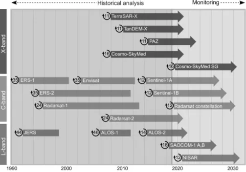
Figure 2.5 shows an overview of the timeline, frequency band, and repeat cycle of most important SAR satellite missions. A rich archive of SAR data is available since the 1990s that is highly valuable for historical analysis. In particular, SAR data provided by ERS-1, ERS-2, and Envisat, the satellites
2.3. SAR Interferometry 21
launched by European Space Agency, made InSAR widely applicable and boosted the development of InSAR techniques and time series analysis in the past years (Ferretti et al., 2001; Berardino et al., 2002). However, SAR data provided by those satellites were temporally sparse, and their coverage was limited to specific regions.
Figure 2.5.: Overview of main SAR satellite missions. The numbers indicate the repeat cycle of the satellites.
High-resolution sensors such as TerraSAR-X and Cosmo-SkyMed broadened the applications of InSAR in detailed displacement mapping particularly in urban and infrastructure monitoring (Perissin et al., 2012; Cigna et al., 2014). These sensors can be tasked to monitor specific areas with high spatial and temporal resolutions. In other areas, however, their background archive is very sporadic.
By the launch of Sentinel-1 in 2014, it has dramatically changed the availability of SAR data. It is the first mission specifically designed to be capable of SAR imaging suitable for InSAR applications.
Sentinel-1 mission regularly acquires medium resolution data all over the world and is planned to continue at least for twenty years (Torres et al., 2012).
2.3. SAR Interferometry
2.3.1. InSAR Workflow
Using two SAR images acquired by a sensor from slightly different locations in space (Figure 2.6), it is possible to form an interferogram by subtracting the phases of the two images. The produced interferogram can be used for two major applications: topography mapping (Zebker and Goldstein, 1986; Rufino et al., 1998; Rossi et al., 2012) and displacement measurement (Gabriel et al., 1989;
Amelung et al., 1999).
22 2. Theoretical Background
Figure 2.6.: Imaging geometry of InSAR in the plane normal to the flight direction. r is the distance between the sensor and the earth surface. θ andθi are the look angle and incidence angle respectively. B is the baseline between the sensor positions at the two times and can be decomposed intoB⊥ and B||. ∆dis the surface deformation occurred between the two times t1 and t2.
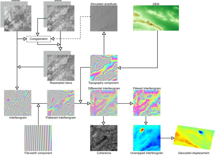
Figure 2.7 outlines the simplified workflow of Differential InSAR (DInSAR) to go from original SAR images to the displacement map. In brief, two SAR images are coregistered and resampled to form the interferogram. Then, flat-earth and topography components are removed from the interferogram, and the so called differential interferogram is generated. After filtering the differential interferogram, its wrapped phase is unwrapped and geocoded (Bürgmann et al., 2000). In the following, different steps of DInSAR workflow are described in more details.
Coregistration defines a mathematical transformation to align the slave image to the master image.
Usually, a low order polynomial can accurately define the transformation model. The transformation parameters are calculated through the least-squares fit of the estimated shifts at different locations over the amplitude images. A coregistration assisted by Digital Elevation Model (DEM) can improve the accuracy (Nitti et al., 2011). Resampling applies the transformation model to slave image and aligns it so identical pixels from master and slave images coincide with each other.
Once the master and slave images are aligned, the interferogram can be generated by multiplying the master image with the complex conjugate of the resampled slave image. The interferometric phase (∆φ) is the coherent sum of components from surface deformation (∆φdef o), flat-earth (∆φf lat−earth), topography (∆φtopo), atmosphere (∆φatmo), and noise (∆φnoise) (Bamler and Hartl, 1998; Rosen et al., 2000; Bürgmann et al., 2000):
∆φ= ∆φdef o+ ∆φf lat−earth+ ∆φtopo+ ∆φatmo+ ∆φnoise (2.1)
2.3. SAR Interferometry 23
Figure 2.7.: Simplified workflow of DInSAR to go from original SAR images to the displacement map.
When the desired component is deformation, other components should be estimated and removed from the interferogram. The flat-earth and topography components are functions of the geometry of the sensor and earth model and can be estimated rigorously. The tropospheric component is either neglected or estimated using the interferometric phase itself or external atmospheric information.
Finally, the remaining noise term is commonly neglected.
The flat-earth component depends on the relative geometry of the sensor at the two acquisition times and the shape of the earth. Therefore, using the precise orbital data and an ellipsoidal model for the earth, usually World Geodetic System 1984 (WGS84), it is possible to estimate and remove this component (Bamler and Hartl, 1998):
∆φf lat−earth=−4π
λ B|| (2.2)
whereλis the wavelength of the SAR system andB|| is the parallel baseline. The interferogram after removing the flat-earth component is so called flattened interferogram.
24 2. Theoretical Background
The topographic component of the interferogram is caused by the elevation of the earth surface from the assumed ellipsoidal model. Using an external DEM, this component is estimated and removed from the interferogram (Bamler and Hartl, 1998):
∆φtopo=−4π λ
B⊥
rsinθi∆h (2.3)
where∆his the surface height from ellipsoid,B⊥is the perpendicular baseline of the interferogram,ris the distance between the sensor and the earth surface, andθiis the incidence angle. The interferogram after removing topography component is so called differential interferogram.
In contrast to flat-earth and topography components, phase contributions from the atmosphere cannot be rigorously estimated. Atmospheric phase delay is a function of physical parameters of ionosphere and troposphere layers. Because precise information on such parameters are not avail- able neither in time nor in space, estimating atmospheric phase is challenging (Hanssen, 2001). The atmospheric artifact is discussed in more details later.
To reduce the noise phase, the interferogram is usually multilooked, which is a spatial averaging of neighboring pixels. Multilooking increases the signal to noise ratio by sacrificing the spatial resolution (Hanssen, 2001). Furthermore, the interferometric phase is filtered to reduce the effect of noise and increase the phase measurement accuracy (Goldstein and Werner, 1998).
After the unwanted components are removed from the interferogram, ignoring the remaining noise, it is assumed that the phase change is caused by surface deformation:
∆φdef o=−4π
λ ∆d (2.4)
where∆dis the surface deformation occurred between the two acquisition times. Because of the cyclic nature of the interferometric phase, only a modulo 2π of the phase values are known. Therefore, it is necessary to recover the integer phase-cycle ambiguity to obtain absolute values in a so called unwrapping process (Goldstein et al., 1988). Afterward, the unwrapped interferogram is geocoded to produce the displacement map.
2.3.2. InSAR Decorrelation
Decorrelation is a major source of noise in InSAR. The phase of master and slave images are correlated if the interaction of the radar echoes with elements within a resolution cell is similar for the two images.
Assuming the thermal noise of the radar system is negligible, there are two sources of interferometric phase decorrelation. First, Significant change of scattering properties, e.g., because of dense vegetation or snow cover, causes temporal decorrelation. Second, slightly different viewing geometries of master and slave acquisitions cause a so called spatial decorrelation (Zebker and Villasenor, 1992).
2.3. SAR Interferometry 25
The similarity of radar echos of masters1and slaves2acquisitions is usually estimated by coherence:
γ = |E[s1s∗2]|
pE[s1s∗1]E[s2s∗2] (2.5)
where ∗ denotes the complex conjugate of a SAR image and E[]is the mathematical expectation. In Practice, because we do not have repeated measurement to estimate the mathematical expectations, values inside a window around a pixel are used to estimate the coherence:
ˆ
γ = |Pn
i=1si1si∗2 | q
Pn
i=1si1si∗1 Pn i=1si2si∗2
(2.6)
It is common to remove the flat-earth and topography components before coherence estimation. An assumption in coherence estimation is that the pixels within the estimation window are statistically stationary (Zebker and Chen, 2005). To satisfy this hypothesis, all pixels within the coherence window should have the same scattering mechanisms.
2.3.3. Errors in InSAR
Atmospheric Error
Atmospheric artifact in InSAR consists of phase delays in ionospheric and tropospheric layers of the atmosphere. Ionospheric phase shift ∆φiono is caused by variations of Total Electron Content (TEC) in the ionospheric layer of the atmosphere and can be approximated by
∆φiono ≈4π k
cf0∆T EC (2.7)
where ∆T EC is the TEC variations in slant direction between the two acquisition times, f0 is the frequency of the traveling signal, c is the vacuum light speed, and k = 40.3 m3/s2 is a constant (Fattahi et al., 2017).
Ionospheric phase change can be estimated and reduced based on internal information in the original SAR data (Jung et al., 2013; Gomba et al., 2016). The delay is proportional to the wavelength of the microwave signal and is severe at high latitudes and equatorial regions (Meyer, 2010). Therefore, the ionospheric artifact is usually neglected for shorter wavelength, i.e., C- and X-band, in mid-latitudes.
The interferometric phase delay due to troposphere ∆φtropo is the difference between the two-way tropospheric propagation delays corresponding to the master φ1tropo and slave φ2tropo images:
∆φtropo =φ1tropo−φ2tropo (2.8)
26 2. Theoretical Background
The two-way tropospheric phase delay of a specific pixel is the integral of the refractivity N, which can be divided into wet and hydrostatic parts, between the height of pixel on the groundh1 and top of tropospherehtop:
φtropo = −4π λ
10−6 cosθi
Z htop
h1
(Nhydro+Nwet)dh (2.9)
Nhydro=K1P
T (2.10)
Nwet =K20 e T +K3
e
T2 (2.11)
where P, T, and e are total atmospheric pressure, temperature, and water vapor partial pressure respectively andk1 = 77.6K hP a−1,k20 = 23.3K hP a−1, andk3 = 3.75·105 K2 hP a−1 are empirical constants (Bekaert et al., 2015a). The hydrostatic part of troposphere depends on the temperature and total pressure, while the wet part depends on temperature and water vapor partial pressure (Delacourt et al., 1998).
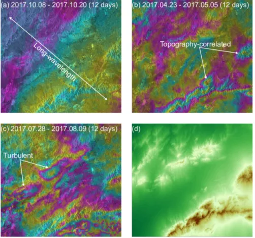
Tropospheric delays are produced by three types of variations in tropospheric parameters. Figure 2.8 shows some examples of interferograms affected by these three types. The first type comes from the broad-scale lateral variations of troposphere (Figure 2.8-a). This type of tropospheric phase delay increases with relative lateral distance. In small interferograms, this effect is corrected by removing a low-order phase ramp. Alternatively, it is estimated using external tropospheric information like global weather models (Jolivet et al., 2011).
The second type of tropospheric artifact in the interferometric phase is caused by vertical variations of water vapor that produces topography-dependent atmospheric delays (Figure 2.8-b). This kind of atmospheric artifact is usually estimated empirically based on the correlation of the interferometric phase with topography or using global weather models (Jolivet et al., 2011).
Finally, short-wavelength turbulent troposphere causes another type of tropospheric delay which is highly variable both in space and time (Figure 2.8-c). Therefore, it is challenging to estimate this kind of tropospheric phase delay (Bekaert et al., 2015a). Reducing this kind of tropospheric delays needs atmospheric information with a high spatial and temporal resolution, for example from dense Global Navigation Satellite System (GNSS) networks.
Remaining DEM and Orbital Errors
As expressed in equation 2.3, the topographic component is proportional to the perpendicular base- line of the interferogram. Therefore, inaccuracies in the DEM appears as errors correlated with the perpendicular baseline:
δφtopo=−4π λ
B⊥ rsinθi
δh (2.12)
2.3. SAR Interferometry 27
Figure 2.8.: Examples of tropospheric effect in different interferograms over a region in the northeast of Iran. All interferograms have 12-day temporal baselines, so it is expected that the magnitude of displacement is small and the interferograms are mostly affected by tropospheric phase delay. (a) the long-wavelength signal (diagonal from top left to bottom right) is caused by
broad-scale lateral variations of the troposphere. (b) the topography-correlated fringes are caused by vertical variations of the troposphere. (c) short-wavelength fringes are caused by turbulent in the troposphere. (d) the topography of the area in the radar coordinate system.
where δφtopo is the phase error caused by topography error δφh. Significant errors in the DEM combined with large perpendicular baselines causes significant remaining topography errors. In case several images are available, by generating interferograms with different perpendicular baselines, it is possible to estimate the remaining DEM error through least square adjustment and correct the interferograms (Fattahi and Amelung, 2013). Because Sentinel-1 is specifically designed to collect SAR images suitable for DInSAR applications, its orbital tube is designed to be narrow. Therefore, the DEM error is less significant for Sentinel-1 in comparison to other sensors (Salvi et al., 2012).
Inaccuracies in the orbital estimation of the satellite results in errors in the estimation of the flat-earth component. Such errors usually appear as a linear trend across the interferogram and are commonly corrected by fitting a linear ramp to the phase change across the interferogram. For older satellites like ERS and Envisat, the ramps caused by orbital inaccuracies are common, but for modern satellites like TerraSAR-X and Sentinel-1, the orbital accuracy is usually enough for a precise estimation of flat-earth component (Fattahi and Amelung, 2014).
28 2. Theoretical Background
2.3.4. Examples of Interferograms
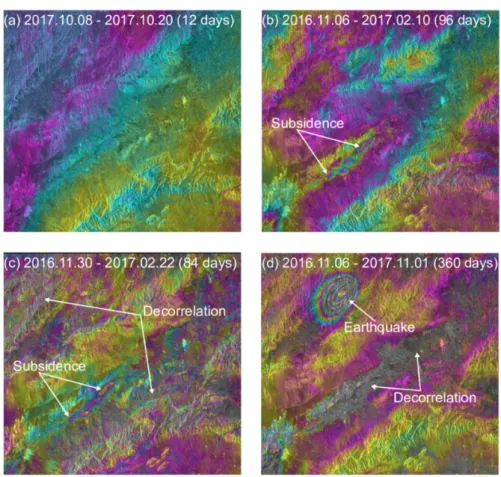
Figure 2.9 shows four examples of differential interferograms with different temporal intervals over a region in the northeast of Iran. The first example (Figure 2.9-a) is a 12-day interferogram with no significant displacement expected in this period. A long-wavelength trend in this interferogram is most likely occurred due to broad-scale lateral variations of the troposphere.
The second interferogram (Figure 2.9-b) covers a 96-day period. This time interval is enough to make localized displacement due to land subsidence visible. The third example interferogram (Figure 2.9-c), which covers 84 days, also shows the subsidence signal. However, Temporal decorrelation has occurred in some areas of the interferogram because of snow cover during the acquisition of 2017.02.22 image.
The last interferogram (Figure 2.9-d) covers a period of 360 days. During the period covered by this interferogram, the 2017.04.05 Mashhad earthquake (Mw 6.1) had occurred. The earthquake fringes are clearly observed in the interferogram. Because of temporal decorrelation due to vegetation cover, the subsidence fringes are obscured by noise.
Figure 2.9.: Examples of interferograms with different temporal separations over a region in the northeast of Iran. (a) a 12-day interferogram does not show any specific deformation feature. (b) Land subsidence features are indicated in a 96-day interferogram. (c) 84-day interferogram exhibits subsidence features. Some areas of the interferogram are decorrelated because of snow cover in the 2017.02.22 image. (d) an approximately 1-year interferogram shows deformation caused by the 2017.04.05 Mashhad earthquake. The subsidence fringes are obscured by temporal decorrelation in the agricultural area.
2.4. Multi Temporal InSAR 29
2.3.5. Decomposition of Line-of-Sight Measurements
InSAR measures the projection of 3-D surface displacement vector on the 1-D line of sight (LOS) vector, which is the direction between the sensor and the ground pixel and is controlled by the incidence angle of the sensor and heading of the satellite. For a right looking sensor, which is the case for most current SAR satellite system, LOS measurement can be expressed as:
∆d= h
Sx Sy Sz i h
∆dx ∆dy ∆dz iT
, (2.13)
Sx=−cosαsinθi Sy = sinαsinθi Sz = cosθi (2.14) where∆dis the displacement of the target pixel in the LOS direction,Sx,Sy, andSz are components of sensitivity vector which defines the sensitivity of LOS measurement to 3-D components of surface displacement (∆dx, ∆dy, and ∆dz). α and θi are the heading and incidence angle of the satellite (Hanssen, 2001).
InSAR LOS measurement is highly sensitive to vertical displacement and the lower the incidence angle, the higher the sensitivity to vertical displacement. The SAR satellites travel in near-polar orbits and conduct measurements perpendicular to their orbits. As a result, the sensitivity of LOS measurements to surface displacement in the south-north direction is significantly lower than the east- west direction. Therefore, it is common to neglect the south-north component and estimate the other two components of displacement by combining the results from both ascending and descending tracks.
In certain cases, it is possible to assume that the displacement takes place in specific directions, particularly in landslide or land subsidence monitoring. In landslide monitoring, it is commonly assumed that the gravity-driven displacement occurs in the slope direction. Therefore, it is possible to estimate the movement direction from the DEM and convert 1-D LOS displacement to 1-D slope movement. In the case of land subsidence, it is common to neglect the horizontal movement and attribute the LOS measurement to vertical displacement. Then, it is possible to estimate the vertical subsidence from InSAR LOS measurements.
2.4. Multi Temporal InSAR
Conventional DInSAR is a powerful method to study large displacements caused by abrupt events like earthquakes. However, when the displacement is within the range of a few millimeters or centime- ters, spanning a relatively long period of time, DInSAR approach faces some difficulties in retrieving the signal mainly because of phase decorrelation and atmospheric artifact. There are different methods developed to analyze the multi-temporal stack of SAR data to overcome the limitations of DInSAR and obtain the history of displacement.
Although they have significant theoretical and practical differences, the common goal of InSAR time series methods is to produce a record of displacement from a collection of SAR data in a few general steps. First, a stack of interferograms is produced. Then, coherent pixels are detected, and their
30 2. Theoretical Background
interferometric phases are connected in time to obtain the time series of displacement. Multi-temporal InSAR analysis approaches are categorized into two general categories: Persistent Scatterer InSAR (PS or PSI) and Small Baseline (SB or SBAS). Each of those categories is optimized for a specific type of scattering mechanisms in SAR images.
2.4.1. Scattering Mechanisms in SAR Images
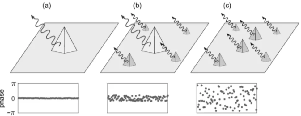
The phase of a pixel in a SAR image is the coherent sum of wavelets from all scattering elements within the pixel (Figure 2.10). Random movements of those elements result in phase changes in repeated radar measurements. In an ideal case for InSAR, the pixel contains only one strong scattering element, e.g., a corner reflector. The level of phase noise for such pixel is very low, and the pixel’s phase is coherent in any combination of SAR images.
In practice, a pixel might contain several scattering elements. If one of the scattering elements within the pixel dominates the other elements, it might preserve enough temporal phase correlation even in interferograms with long temporal and perpendicular baselines. Such a pixel is called a Persistent Scatterer (PS). Persistent scatterers are usually found in urban areas where buildings act as strong scattering elements. Detection of PS points is done at original image resolution, i.e. no multi-looking is applied to the interferograms when analyzing PS points because multi-looking adds more scatterers to a resolution cell (Hooper et al., 2012).
Persistent Scatterers are rare in natural lands where usually a pixel contains several comparable scattering elements. Such pixel is called a Distributed Scatterer (DS). As a result of random movements of the scatterers, the correlation of the pixel’s phase decay quickly. Therefore, distributed scatterers only maintain enough correlation in short-baseline interferograms. It is common to enhance the signal to noise ratio of distributed scatterers by multilooking (Parizzi and Brcic, 2011).
Figure 2.10.: Scattering mechanism for (a) an ideal single scatterer element, (b) a persistent scatterer element, and (c) a distributed scatterer and simulation of temporal phase variations corresponding to each of them.
2.4.2. Interferogram Stacking
Stacking is the simplest approach of multi-temporal InSAR that assumes a linear model for displace- ment and estimates the average rate of displacement from a collection of interferograms. To preserve
2.4. Multi Temporal InSAR 31
the phase correlation of distributed scatterers, the interferograms are generated using image pairs with short temporal and perpendicular baselines. Furthermore, the interferograms are multilooked to enhance the signal to noise ratio. The interferometric phase of a pixel in differential interferogram i can be expressed as (Hooper et al., 2004):
∆φi = ∆φidef o+δφiorb+δφitopo+ ∆φiatmo+ ∆φinoise (2.15) where δφiorb and δφitopo are the phase caused by errors in orbital data and remaining topography respectively. For pixel iinmsample interferograms, the linear rate of displacementvˆis:
ˆ v= 1
m
m
X
i=1
∆φi
BTi (2.16)
whereBiT is temporal baseline of interferogrami(Wright et al., 2001). Stacking works when∆φi has a linear trend in time while other terms in equation 2.15 are stationary in time. Hence, averaging cancels out the random errors and preserves the linear trend of displacement. In reality, violation of this assumption can bias the estimated rate of displacement. Mitigating the errors from atmospheric phase delay, orbital inaccuracies, and remaining DEM, before averaging the interferograms increases the reliability of the estimated rate of displacement (Wang et al., 2009).
2.4.3. Persistent Scatterer InSAR
This approach finds persistent scatterers and performs time series analysis on their phases. Because persistent scatterers preserve a stable phase even in interferograms with large temporal and perpendic- ular baselines, one of the SAR images is selected as the reference. Then, all other images are resampled to the reference image and a star-like network of interferograms is generated (Figure 2.11-a).
Figure 2.11.: An example of interferogram network in (a) Persistent Scatterer InSAR and (b) Small Baseline approaches. The circles and lines represent SAR images and interferograms respectively.
The key step in Persistent Scatterer InSAR is to find pixels containing persistent scatterers. As- suming that a PS pixel demonstrates a low amplitude variation through time, amplitude dispersion DA can be used as a first order test to determine if a pixel is a PS:
32 2. Theoretical Background
DA= σA
µA (2.17)
whereσAandµAare standard deviation and average of amplitude values for a specific pixel in a stack of the interferogram (Ferretti et al., 2001). Once the initial set of PS candidates are selected, their temporal phase behavior is analyzed to estimate the noise level of each pixel. The final set of PS pixels is formed from the pixels that exhibit a subtle level of phase noise. To estimate the noise level
∆φinoise, other phase contributions should be estimated and removed from equation 2.15.
There are two main approaches to estimate the noise level of a pixel. The first approach utilizes the double phase difference between neighboring PS candidates (Ferretti et al., 2001; Kampes, 2005).
Because atmospheric and orbital errors are spatially correlated, they are removed in the double differ- ence phase. DEM error is estimated from the correlation of phase with perpendicular baselines in the stack of interferogram. Finally, the displacement is estimated by using a predefined model, usually linear or sinusoidal. The remaining noise for double difference phases is adjusted to estimate the noise level of each pixel (Hooper et al., 2012). This method is mostly applicable in urban areas where many buildings act as stable scatterers. The main drawback of this approach is that it needs a predefined displacement model; deviations from the predefined displacement model cause falsely high estimation of noise, and hence less number of PS pixels are selected.
There is another approach to estimate the noise level in a stack of interferograms without any predefined displacement model (Hooper et al., 2004). In this approach, it is assumed that contributions from deformation, atmosphere and orbital error in equation 2.15 have low spatial frequencies and therefore are estimated by spatial filtering. The remaining DEM error which has a high spatial frequency can be estimated from its correlation with perpendicular baseline. After removing all these contributions, the noise phase is the only remaining component in equation 2.15. In comparison to the former methods, this approach provides a higher density of detected persistent scatterers in non-urban areas (Hooper et al., 2012).
Once the persistent scatterer pixels are selected, their phases are unwrapped and connected tem- porally to obtain the time series of displacement. Then, the unwanted components like tropospheric artifact are estimated and removed from the time series by spatial and temporal filtering. Further- more, the remaining DEM errors are modeled and removed based on the correlation of unwrapped phases with perpendicular baselines.
2.4.4. Small Baseline InSAR
In Small Baseline approach, a network of interferograms is generated with short perpendicular and temporal baselines to minimize the spatial and temporal decorrelations of distributed scatterers (Figure 2.11-b). In this approach, the pixels are usually selected based on their coherence values. By setting a threshold, pixels with high coherence in a given percentage of interferograms are included in the processing (Berardino et al., 2002).
2.5. Analysis of Displacement Time Series 33
To increases the signal to noise ratio of phase values in the interferograms and hence the chance of finding reliable DS pixels, the SB interferograms are usually multilooked. However, multi-looking decreases the resolution of the interferograms and smears isolated coherent pixels surrounded by noisy pixels. To overcome this, a statistical phase analysis similar to Persistent Scatterer InSAR can be performed to select pixels at original interferogram resolution (Hooper, 2008).
After the reliable pixels are detected, their phases are unwrapped either in 2 dimensions in each interferogram independently or jointly using time as the third dimension (Berardino et al., 2002;
Hooper, 2008). Then, the unwrapped displacement of different interferograms in the network are inverted to solve the displacement at each date. If ∆dti1,t2 is the displacement in ith interferogram between dates t1 andt2, a linear system withm equations corresponding to each inteferogram and n unknowns corresponding to each SAR date is formed for each pixel as follows:
Am,nXn,1 =Lm,1 (2.18)
WhereAis filled with−1and1for elements corresponding to master and slave images respectively and 0 otherwise. L contains the displacement values of a pixel in all SB interferograms. X is the unknown displacement at each SAR date and is solved by minimizing the Lp norm of residuals:
Xˆ = arg minkL−AXkp = arg min
m
X
i=1
|L−AX|pi
1 p
(2.19)
AL2−normminimization provides the solution:
Xˆ = (ATA)−1ATL (2.20)
After estimating the time series of displacement, as the final step of Small Baseline processing, DEM error is estimated by considering its correlation with perpendicular baseline and the atmospheric artifact is filtered out from the time series by spatial and temporal filtering.
2.5. Analysis of Displacement Time Series
Displacement time series obtained from Multi Temporal InSAR can be further examined to inves- tigate significant temporal features and their link to their causes. Mathematical tools such as Fourier transform and Wavelet transform provide information about periodicities in the time series. The for- mer method determines frequencies in a stationary time series but does not give information about the time of occurrence. In contrast, wavelet transform yields a time-frequency representation of the signal to detect periodicities and locate them in time.
34 2. Theoretical Background
Wavelet transform has been used extensively for decades in different geophysical applications (Foufoula-Georgiou et al., 1994; Chakraborty and Okaya, 1995; Martelet et al., 2001; Hetland et al., 2012). There are two classes of the wavelet transform. Discrete wavelet transform is mostly used in noise reduction and image compression, while Continuous Wavelet Transform (CWT) is used for feature extraction (Grinsted et al., 2004).
2.5.1. Continuous Wavelet Transform
Convolution of a time series (xn, n = 1, ..., N) with a wavelet function ψ0(η) gives the continuous wavelet transform:
WnX(s) = rδt
s
N
X
n0=1
xn0ψ0
(n0−n)δt s
(2.21)
wheres is the scale that defines the width of wavelet and δt is the time step for sliding the wavelet along the time series. Morlet, one of the wavelet functions frequently used in geophysical applications is defined as:
ψ0(η) =π−14eiω0ηe−12η2 (2.22) whereω0 and η are the dimensionless frequency and time, respectively. The wavelet power spectrum
|WnX(s)|2 provides information on periodicities at different scales through the time (Torrence and Compo, 1998).
2.5.2. Cross Wavelet Transform
It is possible to jointly analyze time seriesxnandynin time-frequency space to examine their relation- ship. Cross Wavelet Transform (XWT) of the two time series, defined as WXY(s) = WX(s)WY∗(s) where∗represents complex conjugate, provides information on the link between the time series. XWT can be decomposed into amplitude and phase as:
WXY(s) =
WXY(s)
eiΦj(s) (2.23)
where the amplitude
WXY(s)
represents the cross-wavelet power and the phaseΦj(s)represents the time lag between two time series at different scales through time (Torrence and Compo, 1998; Maraun and Kurths, 2004).
2.5. Analysis of Displacement Time Series 35
2.5.3. Application of CWT and XWT to InSAR Time Series
The CWT and XWT can be applied to any time series that is evenly distributed in time; InSAR time series do not usually satisfy this rule, however. Therefore, before performing the time-frequency analysis, the displacement time series should be interpolated to uniformly-spaced intervals. Time series of other geophysical measurements such as rainfall and groundwater level should be interpolated to similar intervals. Applying CWT on the interpolated time series reveals periodicities at specific scale and specific time. Then, common frequencies and the time lag between the time series can be identified by XWT.
Chapter 3
Methodological Contribution
38 3. Methodological Contribution
3.1. Introduction
Sentinel-1, launched in 2014, is the first SAR satellite mission to provide regular SAR acquisitions all over the globe. This mission is specifically designed to provide SAR data suitable for InSAR applications. Its moderate resolution and extensive coverage make it a great candidate for InSAR observation for many applications. Although Sentinel-1 offers a new opportunity for monitoring dis- placement regularly over broad areas, it brings new challenges that have to be addressed to be able to extract relevant information from the data.
There have been successful attempts in the past few years in order to adapt the already established InSAR processing methods, split the data into several chunks and process them in parallel. Such approaches can be implemented in cloud computing platforms to provide reliable results over extensive areas (Luca et al., 2017; Zinno et al., 2018). The main aim of this chapter is, however, to give a new undemanding workflow that benefits from the massive stream of Sentinel-1 data to effectively reduce the errors and provide reliable time series of displacement.
3.2. Challenges in Large-scale InSAR
There are several challenges in large scale InSAR analysis that need to be addressed. The first challenge is the large amount of data and the need for efficient workflows that are computationally affordable. Furthermore, the workflow should work with minimal operator interactions. It is not the case in many sophisticated approaches that need the operator to observe and control the processing chain carefully.
The second challenge of large-scale InSAR processing is to specify the appropriate reference area.
InSAR measures displacement with respect to an arbitrary reference area. The reference is usually selected as close as possible to the region of interest, so the spatially correlated nuisance phases in the reference area are approximately similar to the region of interest. Therefore, subtraction of the reference area’s phase removes parts of spatially correlated noises. As the distance between the reference point and the region of interest increases, the error propagated between them increases (Fattahi and Amelung, 2015).
External information from independent geodetic measurements can help a reliable selection of ref- erence areas. In many cases, InSAR measurements are constrained by external measurements, e.g.
from GNSS, but such information is not available in many areas. When such data are not available, it is common that the operator visually inspects the results and selects the reference point in an area close to the study area that is assumed to be free of displacement. However, visual inspection is time-consuming and inefficient as the scale of data grows. Therefore, an automatic selection of the reference area is needed in order to obtain homogeneous and reliable information.
Finally, the spatially propagated errors cause significant phase biases in the regions far from the reference area. The errors should be reduced as much as possible in order to obtain reliable dis- placements. Tropospheric artifact is the major source of error that biases the phase difference over the large distances. The relationship between phase and topography or external information such as