Structure and variability of the circulation at tidal to intra-seasonal time scales near

(1)

University of Bremen

Alfred Wegener Institute, Helmholtz Centre for Polar and Marine Research

Structure and variability of the circulation at tidal to intra-seasonal time scales near

the 79 North Glacier Master thesis

submitted in

Postgraduate Programme Environmental Physics

Author:

Luisa von Albedyll Matr. No: 3031314

Supervisors:

Prof. Dr. Torsten Kanzow Prof. Dr. Monika Rhein Tutor:

Dr. Janin Schaer

Bremen, 18.10.2018

(2)

Abstract

Greenland's largest oating ice tongue at the Nioghalvfjerdsfjorden Glacier (79 North Glacier) is thinning, most likely triggered by enhanced submarine melting. The strength of the cavity circulation beneath the oating ice tongue is essentially responsible for the ocean heat ux to the glacier ice and variability in the circulation may have consequences on the basal melt rate. Analyzing four moored records (summers 2016-2017) from the 79 North Glacier calving front, this study characterizes the variability of the cavity circulation and the relative importance of its local and regional drivers. The focus lies on the variability in the currents in Dijmphna Sund, the most relevant export pathway for glacially modied waters out of the glacial cavity. Variability is split into three groups. (1) Half of the variance of the time series is concentrated at sub-daily to daily time scales (T= 0.25−2 days) and is associated with barotropic tides. (2) Periods of 2-30 days comprise one third of the variance. At those time scales, currents in Dijmphna Sund are weakly linked to sea ice conditions close to the coast and enhanced wind speeds. (3) In periods larger than 30 days,¹/6of the variance is found. Low-pass ltered Empirical Orthogonal Functions reveal a strong link between the export of glacially modied waters through Dijmphna Sund and the inow into the glacial cavity. This intra-annual variability of the cavity circulation was also observed by a mooring on the continental shelf 170 km south of the 79 North Glacier. The time series from the calving front and the one from the continental shelf are signicantly correlated (R= 0.65) and shifted by a time dierence of 27 ±29 hours. The time delay ts well to travel times of baroclinic waves. This suggests that large-scale wave activity may be the main driver of the intra-annual variability of the cavity circulation.

(3)

1 Introduction

1.1 Ocean-glacier interactions in Greenland

Polar ice sheets play an important role in the climate system. Fluctuations in their mass balance have shaped past climatic changes substantially. For example, sea level has risen since the last glacial maximum, i.e., about 20,000 years ago, by over 120 m as a result of mass loss from the ice sheets (e.g., Church et al., 2013). Further, anomalous freshwater contributions during the disintegration of the Laurentide ice sheet covering North America are suspected to have caused the Younger Dryas, a rapid cooling event on the Northern Hemisphere associated with a reduced Atlantic Meridional Overturning circulation (Fair- banks, 1989).

The current sea level rise of 3.1 ± 0.3 mm yr⁻¹ observed over the last two decades is attributed to ocean thermal expansion (42%) and melting of land ice (58%). The loss of land ice is distributed onto glaciers (21%), the Greenland ice sheet (15%) and the Antarctica ice sheet (8%, Nerem et al., 2018; WCRP Global Sea Level Budget Group, 2018). Satellite observations show that the Greenland Ice Sheet loses mass since the early 1990s and that the loss has quadrupled over the past two decades (Enderlin et al., 2014;

Shepherd et al., 2012). With respect to sea level, the Greenland Ice Sheet contributed between 2012 and 2016 at a rate of 0.67 mm yr⁻¹ (Bamber et al., 2018). Climate models predict an an additional contribution from the Greenland Ice Sheet to global sea level rise of 54-97 mm until the end of the century for a 1.5°C warming szenario (Marzeion et al., 2018).

Widespread retreat and speed-up of marine terminating glaciers, as well as increased surface runo due to higher surface temperatures are responsible for the observed mass loss of the Greenland Ice Sheet. A large portion of the enhanced ice ux to the ocean is most likely triggered by increased submarine melting at marine-terminating glaciers (e.g., Hill et al., 2017; Kjeldsen et al., 2015; Straneo and Heimbach, 2013). Subsequent thinning and accelerated retreat destabilize glaciers and ice shelves and may cause enhanced mass loss. Thus, since the ocean circulation determines the heat ux to the glaciers, a better understanding of the temporal variability of the ocean circulation is of great relevance to improve our predictions of the future contributions to sea level rise from the Greenland Ice Sheet.

Besides sea level rise, increased freshwater release impacts the regional, and most likely the global ocean circulation. Increased ice loss from the Greenland ice sheet contributed to a freshwater anomaly in the North Atlantic Ocean, reaching a total volume of∼3200 km³ for the time period 19922010 (Bamber et al., 2012). A substantial fraction of melt water from Greenland intrudes the ocean at depth and mixes with ambient water (Straneo et al., 2011).

When exported o the continental shelf, increased freshwater input is particularly relevant because Greenland's coast is located in the proximity of the North Atlantic dense water formation sites (Dickson et al., 2007). Modeling studies showed that especially melt water from east Greenland reaches the interior of Labrador Sea and may impact the stratication at the convection sites (Dukhovskoy et al., 2016; Gillard et al., 2016). However, it is not well understood yet how the increased melt water alters the Atlantic meridional overturning circulation. Some models suggest a reduction (e.g., Böning et al., 2016; Weijer et al., 2012),

(6)

but especially the inuence of parameters like runo location, exact amount and intrusion depth are not well known and only sparsely supported by observations (Dickson et al., 2007;

Gillard et al., 2016). Consequently, an improved understanding of the glacial freshwater discharge into the ocean is required to predict the ocean's response to the enhanced ice loss at the Greenland Ice Sheet more realistically.

Key regions to better understand the interactions of the open ocean and marine-terminating glaciers are the glacial fjords around Greenland. Normally, two type of water masses are found in them: light waters of Arctic origin, called Polar Water (PW) and dense, warm waters of Atlantic origin (Straneo and Cenedese, 2015). Providing a pathway for the Atlantic water, they steer the ow of warm water to the glacier calving fronts. The dynamics of the fjord's circulation determine the heat transport to the glaciers and the glacial freshwater export to the continental shelf. Within the fjords and on the continental shelves, glacial freshwater may be transformed (e.g., by mixing with waters of Polar or Atlantic origin) before it may modify the hydrographic properties on the continental shelf.

Consequently, knowledge of the fjord's dynamics is an important piece to understand ocean- glacier interactions. The fjord's circulation is assumed to result from a combination of dierent drivers, that interact and exhibit variability at dierent time scales (Cottier et al., 2010; Straneo and Cenedese, 2015; Sutherland et al., 2014a). The most common ones are listed below:

(1) The buoyancy-driven circulation is forced by thermohaline dierences. It outputs fresher water at shallow depths and subsequently draws in more saline water at depth (Motyka et al., 2003). The buoyancy-driven circulation is maintained by supply of melt water, i.e., either subglacial runo (melted at the surface) or basal melt (melted at the ocean-ice interface). Melting along the glacier front (or below a glacial tongue) is strongest at depth, i.e., where the glacier is in contact with the warmest waters. In addition, rising freshwater plumes entrain on their ascent ambient water and thereby enhance the heat transfer until they reach neutral buoyancy. In strongly stratied fjords this level is often reached at the lower limit of the light and cold PW that occupies the upper 100-150 m of the water column (Straneo and Cenedese, 2015; Straneo et al., 2011). The buoyancy- driven circulation is thought to be enhanced during summer, because more freshwater is discharged at the grounding line compared to winter when it is driven by basal melt only (Straneo et al., 2011).

(2) Shelf-driven intermediary currents in fjords are induced by density uctuations at the fjord's mouth. The density gradients between fjord head and mouth can be induced by any forcing, but are often associated with along-shore winds that pile up water at the fjord's mouth inducing downwelling (Jackson et al., 2014; Straneo et al., 2010). This leads to a ow into the fjord in the upper layer and a ow out of the fjord at depth, resulting in a depressed pycnocline within the fjord (Klinck et al., 1981). When the winds calm down and the outer shelf returns to the pre-event state, the circulation reverses (Straneo et al., 2010). Those pulses are associated with strongly sheared, fast ows that reverse in depth and time with a typical duration of 4-10 days (Jackson et al., 2014). When forced by winds, it is expected that the seasonal strength of the intermediary currents is linked to the wind speeds. Waves communicating disturbances in the pycnocline were also shown to initialize a similar intermediary fjord circulation (Inall et al., 2015).

(3) Along-fjord winds inuence the fjord circulation (e.g., Cottier et al., 2010; Klinck et al., 1981). A model by Klinck et al. (1981) showed that surface circulation can be closely correlated with the winds directed along the fjord, that may be, however, overridden by an intermediary circulation (if present). Moat (2014) showed that in a Patagonian fjord with a shallow sill the local along-fjord wind-driven circulation dominates. During down-

(7)

fjord wind events, the existing estuarine circulation is intensied, but during up-fjord wind events the inow of deep water is signicantly reduced and a three-layer exchange ow develops.

(4) Mixing introduced by a variety of processes may lead to water mass modication. In case of vertical mixing, the density stratication will be changed, potentially inducing a mean motion. Wind stress is the dominant driver of mixing in the upper ocean (Cottier et al., 2010). Sea ice enhances the momentum transfer between atmosphere and ocean as long as the oats still move around. Martin et al. (2014) found an optimal concentration for increased momentum transfer into the ocean at 80-90% of ice coverage. While sea ice is formed, brine release can induce convective overturning. During times of a closed sea ice cover, other processes like tides can act as exchange agents. For instance, Kirillov et al. (2017) observed tides to transport subglacial water from the Flade Isblink Glacier to the continental shelf. In case of silled fjords, tides can cause shelf-fjord exchange ow, introducing a net salt transport and establishing a fjord circulation ("Tidal pumping", see Boone et al., 2017). Apart from tides, low-frequency baroclinic waves can provide kinetic energy for mixing (Sutherland et al., 2014a).

The dynamics of glacial fjord's in Greenland has been subject of an increasing number of recent studies (see Straneo and Cenedese, 2015, for a review), but there are still major gaps in understanding the circulation because observations are limited due to logistical challenges of the remoteness of the glacial fjord systems and a semi-permanent sea ice cover (Sutherland et al., 2014a). Most studies focus on fjords in Southern Greenland that reach to tidewater glaciers, for example from west to southeast, Kangia Ice Fjord/Jakobshavn Isbræ(e.g., Motyka et al., 2011), Godthåbsfjord (e.g., Mortensen et al., 2011), and Sermilik Fjord/Helheim Glacier (e.g., Jackson et al., 2014; Straneo et al., 2010). Recently, a number of studies focused also in glacial fjords located North Greenland. Studies on Flade Isblink Ice Cap (Northeast Greenland, 81 °N) explored hydrography, inuence of tides and storms and proposed that the outlet glacier has a oating ice tongue (Bendtsen et al., 2017;

Dmitrenko et al., 2017; Kirillov et al., 2017). Additionally, circulation at Petermann's glacier that has an extensive ice tongue and is located in North Greenland is described by, e.g., Johnson et al. (2011) and Washam et al. (2018).

A few wintertime records give some rst insights into the seasonality of the fjord circulation (Boone et al., 2017; Jackson et al., 2014; Mortensen et al., 2013), stressing the need of year-long observations (Straneo and Cenedese, 2015). This study presents a compre- hensive oceanographic data set from the fjord covered by the 79 North Glacier, located in Northeast Greenland. In total, four moorings monitored for seven to twelve months the gateways of the cavity circulation beneath the largest oating ice tongue Greenland's.

Those measurements will shed light on the fjord circulation and its seasonal variability near the 79NG. Eventually, those observations will most likely help to improve the general understanding of fjord circulation in Greenland's fjords.

1.2 Ocean inuence on the 79 North Glacier

Satellite observations have demonstrated that between 2009 and 2012 60% of the increased mass loss of the Greenland Ice Sheet is forced by enhanced surface runo and 40% by ice discharge from outlet glaciers that drain the Greenland Ice Sheet (Enderlin et al., 2014;

van den Broeke et al., 2009). A large part of Northeast Greenland (approximately 12%

of the Greenland Ice Sheet, Mouginot et al., 2015) is drained by the Northeast Greenland Ice Stream (NEGIS), an elongated, narrow region of enhanced ow velocities that reaches deep into the ice sheet (Fig. 1.1 and 1.2, Joughin et al., 2001). Having remained close

(8)

East Greenland Current

Greenland

AIW

glacier velocities

0 km yr¹ 11

West Spitsbergen Current

1000 500 250 100 0

Bathymetry (m)

Figure 1.1: Green- land Ice Sheet glacier speeds and major ocean currents in Fram Strait. Warm Atlantic water is transported in the West Spitsbergen current to the Arctic and recir- culates in Fram Strait.

At the continental shelf break, it is modied to Atlantic Intermediate Water (AIW) and transported to the 79NG.

The glacier velocities (provided by ESA) show the 79NG as one outlet of the North East Greenland Ice Stream.

to equilibrium over the last century, the NEGIS seems to respond in more recent years to changes in the climate forcing. Increased surface runo and enhanced ice discharge via the outlet glaciers of the NEGIS, named Nioghalvfjerdsbræ, Zachariæ Isstrøm and Storstrømmen are the suspected drivers of the observed dynamical thinning (Khan et al., 2014; Mouginot et al., 2015). The oating ice tongue of Zachariæ Isstrøm disintegrated between 2003 and 2012 what lead to an increase in ice discharge by 50% between 1976 and 2015 (Mouginot et al., 2015). The direct neighbor of Zachariæ Isstrøm is Nioghalvfjerdsbræ (Danish for 79 North Glacier, hereafter 79NG). The 79NG has the largest remaining ice shelf in Greenland (70 km long, 20 km wide, Fig. 1.3) whose surface area was remarkably stable. Pinning points at the glacier calving front and upwards sloping bedrock at the grounding line seem to stabilize the glacier. However, recent studies indicate that the oating tongue of the 79NG lost 30% of its thickness from 19992014 (Mouginot et al., 2015; Wilson et al., 2017). Mayer et al. (2018) showed that the 79NG is out of mass balance equilibrium since 2001. Models predicts a retreat of the grounding line of approximately 10 km within the next 80 years and further thinning of the oating ice tongue (Choi et al., 2017; Mayer et al., 2018). Considering that thin ice is less stable, a disintegration of the ice shelf is likely (Mayer et al., 2018). The mass balance of the 79NG is dominated by submarine melting that accounts for 80% of the annual mass loss when excluding the rare calving events (Reeh et al., 2001; Wilson et al., 2017). Mayer et al. (2018) attribute the thinning and its large variability to an increased basal melt due to enhanced heat ux from the ocean. The subglacial melting is triggered by the presence of warm Atlantic waters in the subglacial cavity (Schaer et al., 2017; Wilson and Straneo, 2015). This water mass of Atlantic origin has been observed to warm by 0.5°C in front of the 79NG since the late 1990s (Schaer et al., 2017). The important role of the ocean to the thinning of the glacier tongue, rises the need for a better understanding of the variability in the oceanic energy ux to the glacier. As summarized above, the glacial fjord circulation is driven by forcing on dierent time scales and knowledge of those is crucial to understand the temporal variability of the ocean's impact on the 79NG. This thesis intents to contribute to this overarching aim by characterizing variability on time scales shorter than one year of the complex fjord circulation. In the following, a brief overview is given over the known

(9)

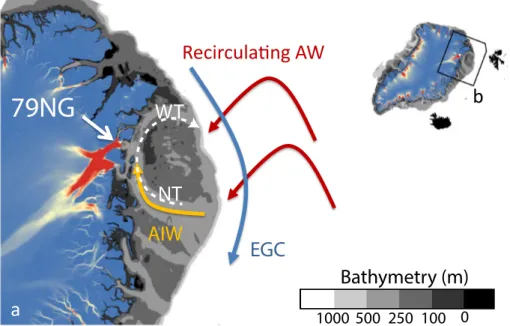
Recircula�ng AW

79NG

AIW EGC NT

WT b

a

1000 500 250 100 0

Bathymetry (m)

Figure 1.2: Ocean circulation close to and on the Northeast Greenland continental shelf. a, Close-up of the Northeast Greenland continental shelf. The East Greenland Current (EGC) transports light Polar Water and recirculated AW along the continental shelf break towards the south. Recirculated Atlantic Water enters the continental shelf and is modied to Atlantic Intermediate Water (AIW). AIW travels in Norske Trough (NT) northwards to the 79NG. The surface circulation (0-200 m deep) is characterized by an anti-cyclonic gyre (white arrow), following the trough system of Norske Trough and Westwind Trough (WT) (Budéus and Schneider, 1995;

Schaer et al., 2017). b, the black rectangular indicates the region of Greenland displayed in a.

aspects of the hydrographic properties and circulation at the 79NG (Section 1.3). Finally, the focus and concept of this thesis is presented in Section 1.4.

1.3 Hydrographic properties and cavity circulation near the 79 North Glacier

1.3.1 Water masses near the 79 North Glacier

The 79 North glacier is in contact with warm waters of Atlantic origin via a trough system on the Northeast Greenland continental shelf (Fig. 1.1, 1.2, Schaer et al., 2017). This warm water mass originates from (1) recirculated Atlantic Water (RAW) that is found at the continental shelf break at the entrance of the southern trough (Norske Trough) and (2) modied Arctic Atlantic Water that has been cooled and freshened in the Arctic and is mainly present at the entrance of the trough located to the North (Westwind Trough, 1.2 Richter, 2017; Rudels et al., 2005; Schaer, 2017). When mixed onto the continental shelf, the Atlantic water undergoes major transitions leading to a pronounced cooling. Both water masses, transformed RAW and AAW are grouped together under the term Atlantic Intermediate Water (AIW) (Bourke et al., 1987; Schaer et al., 2017). The warmer part of the AIW is transported via Norske Trough into the 79NG bay, most likely following a continuous pathway deeper than 300 m to the calving front (1.2 Schaer, 2017).

AIW being warmer than 1 °C enters the 79NG cavity through a deep channel in front of the main terminus of the 79NG (1.3, Fig. 1.4, and 1.5) carrying enough heat to melt glacier ice (Schaer, 2017). Most of the melting takes place at the grounding line, where the glacier is in contact with the warmest water (e.g., Mayer et al., 2000; Wilson and Straneo, 2015).

(10)

Melting occurs in two steps. The ocean heats up the ice to the freezing-point potential temperature that depends on pressure. Then, it further provides the latent heat necessary for the phase change from solid to liquid. As the ocean provides the heat for warming and melting the ice at the glacier base, it cools as result. Basal melt is released which mixes with the ambient water inside the glacier cavity to form a mixture that is fresher and lighter compared to the inowing AIW (Straneo and Cenedese, 2015).

Additionally, subglacial runo that has drained through cracks and englacial channels to the glacier bed is discharged at the grounding line. Mixing of AIW, basal melt and subglacial runo forms a plume that is lighter than the surrounding water and ascents along the ice base until it reaches neutral buoyancy. Further mixing with ambient water leads to the formation of glacially modied Atlantic water (mAIW) that leaves the cavity at intermediate depths (approx. 90-250 m).

Using current, potential temperature, and salinity measurements from the main calving front of the 79NG in summer 2016, Schaer (2017) found, that AIW has potential densities of 27.75 to 27.9 kg m⁻³ and temperatures between 0.7 and 1.3 °C in front of the calving front (Fig. 1.4, Fig. 1.5). Such warm water was present only at two of ve channels along the glacier calving front (Fig. 1.4).

The mAIW between 120 and 270 m covered a density range between 27.0 and 27.75 kg m⁻³, corresponding to temperatures between -0.5 and 0.7 °C. An Optimum Multiparameter analysis (OMP, see Section 2.1.3 and appendix) based on potential temperature, salinity and dissolved oxygen revealed that in 2016 the mAIW consisted on average of approximately 2% glacial melt water (see Fig. 1.5). Basal melt water accounted for three quarters of the total melt water content (Fig. 1.4, Fig. 1.5). The highest melt water concentrations were present in Dijmphna Sund (Fig. 1.5), i.e., the fjord extending from the minor calving front to the northeast (Fig. 1.3) . Further on the continental shelf, the signature of mAIW becomes less pronounced, possibly induced by mixing with ambient water masses (Schaf- fer, 2017). The upper part of the main pycnocline is formed by PW that exhibits low salinities at potential temperatures close to the freezing point (Fig. 1.5). PW is probably transported from the Arctic ocean onto the continental shelf and not locally formed which is suggested by its nutrient signature that points to a Pacic origin (Falck, 2001).

1.3.2 Glacial cavity circulation of the 79 North Glacier

Water exchange across the glacial calving front involves four distinct pathways shaped by the complex bathymetry close to the 79NG (Fig. 1.2, 4.6, Schaer, 2017). All pathways were monitored between summers 2016 and 2017 by moored measurements. While the cavity beneath the oating tongue is deeper than 900 m (Mayer et al., 2000), the bathymetry slopes upwards towards the main calving front, so that the glacier is grounded over a large area. The deepest bathymetric channel and the main gateway for inow is located between the islands A and the pinning point B (monitored by mooring M2). Here, a 500 m deep depression slopes down into the glacier cavity (Fig. 4.6, Schaer, 2017). Towards the south, there are two more pathways of approximately 300 m depth. The rst is located between pinning point B and C (mooring M3) and the second between pinning point D and the coast of Lamberts Land (M4). The bathymetry of the 300 m deep passage is complex and might include a sill of 280 m depth towards the glacier (Schaer, 2017). At the northern, minor calving front that joins into Dijmphna Sund, no such complex bathymetry is known, but the ow is blocked by a 170 m deep sill at the fjord's mouth where mooring M1 was placed (Fig. 1.2).

Wilson and Straneo (2015) proposed that the cavity circulation of the 79NG is a buoyancy- driven estuarine exchange ow, i.e., a circulation mainly determined by the freshwater

(11)

CTD sta�on Mooring 2016-2017

5 cm/s A

B D C

a b

-450 m -250 m -50 m

A pinning point

Grounding line

Bathymetry

Hovgaard Ø

79 NG

Dijmphna Sund

Lambert Land

Figure 1.3: Glacial cavity circulation of the 79NG. a, locations of measurement stations (CTD and Mooring M1-M4) at the 79NG calving front and in Dijmphna Sund are displayed. At each mooring site (star), the direction of the strongest ow is indicated by a yellow (ow directed into the cavity) or white (ow directed out of the cavity) arrow. b, close-up to the main calving front (see white rectangular in a for extent indicator). The channels to the cavity are located between the pinning points A-D

M4 M3 M2

Figure 1.4: Potential Temperature section at the main cavity calving front of the 79NG in summer 2016 during the CTD survey. AIW is present in the cannel between pinning point A and B and between D and the southern coast. Isopycnals are overlain as black lines. Figure adapted from Schaer (2017).

(12)

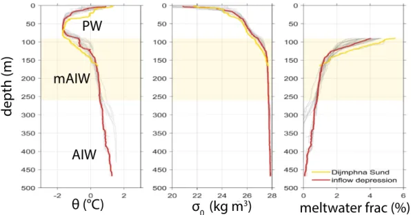
PW mAIW

AIW

depth (m)

θ (°C) σ

₀

(kg m

³

) meltwater frac (%)

Figure 1.5: Potential temperature, salinity and meltwater content proles in 2016 for CTD casts at the calving front and in Dijmphna Sund in 2016. a, potential temperature prole with indications of water masses. Atlantic Intermediate Water (AIW), glacially modied AIW (mAIW) and Polar Water (PW). A prole taken in Dijmphna Sund (yellow) and one from the inow depression (red) is highlighted. The depth range in which most outow is observed is shaded in yellow. b, potential density. c, melt water fractions beneath 90 m calculated based on an end-member analysis (see Section 2.1.3 and appendix)

supply via basal melting and surface runo in which inow takes place as compensation of the export of fresher water. Schaer (2017) suggested that the inow is additionally hydraulically controlled. Her analysis showed that the bottom-intensied ow that transports AIW into the glacial cavity is associated with a gravity plume that is descending the sill located to the north of shallow bank close to the inow depression. The density dierences between upstream and downstream of the sill arise due to the presence of glacially modied waters in the downstream basin that induce buoyancy gain via mixing. The hydraulically controlled ow is very sensitive to the bifurcation depth, i.e., the height of the AIW layer above the sills that might be inuenced by tides, storms, deep convection due to seasonal variability and advected long-term changes (Schaer, 2017).

Balanced transport estimates based on the moored observations weight the relative importance of the dierent gateways (Fig. 1.6, Schaer et al 2018, in prep). Inow of 52 mSv takes place exclusively at the inow depression (M2) below approx. 240 m. Export is distributed over Dijmphna Sund (-24 mSv) and all other three gateways at the main calving front, i.e., M2 (-13 mSv), M3 (-12 mSv) and M4 (-3 mSv). Dijmphna Sund accounts for almost half of the export and outweighs each of the pathways by almost the double export.

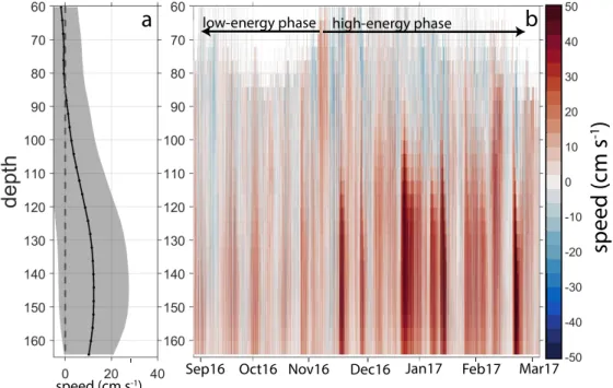
Former studies have estimated the role of Dijmphna Sund to be of minor relevance. Wilson and Straneo (2015) calculated geostrophic ow velocities of less than 0.3 m s⁻¹ below 80 m depth at the mouth of Dijmphna Sund. Furthermore, a moored current meter placed at the glacier rift close to the Dijmphna Sund calving front measured prevailing currents directed to the West, i.e., away from Dijmphna Sund (Schaer, 2017). Indeed, the time series recorded at Dijmphna Sund reveals a strong temporal variability, with velocities varying between 0.1 m s⁻¹ and 0.7 m s⁻¹ that may explain why single current measurements did not yet capture the fast velocities.

Dijmphna Sund was picked as a suitable start location to study the glacial fjord circulation at the 79NG. Besides the large volume export of mAIW, the melt water fraction analysis

(13)

a

b c

M4 M3 M2 M1

M4 M3 M2 (out) M1 M2 (in)

Figure 1.6: Velocity measurements of LADCP survey and balanced transport estimates from moorings. a, velocity section of the four gateways to the glacial cavity from south to north, calculated based on LADCP proles (triangles) and mean proles from the moored measurements (circles). Isotherms (yellow lines) and ispycnals (black lines) are overlaid. The cross sections of the channels were used as displayed to calculate transports, displayed in b. b, prole of the mean transports for the moorings M1-M4 (Aug 2016-Mar2017). c, stream function of the transport; once calculated including Dijmphna Sund (period Aug2016-Mar2017) and excluding Dijmphna Sund (period Aug 2016-Sep 2017). Figure provided by J. Schaer (personal communication, 2018).

indicated that melt water concentrations were highest, i.e., not only the most, but also the freshest mAIW is exported here (Fig. 4.8). Considering that mAIW higher up in the water column contains more freshwater, and taking into account that mAIW export at Dijmphna Sund takes place at more shallow depths than compared to the main calving front, Dijmphna Sund distributes not only the most mAIW, but also the most freshwater.

Fjord processes modifying the circulation in Dijmphna Sund are therefore of high relevance for the freshwater export from the 79NG to the continental shelf. Furthermore, Dijmphna Sund is located about 75 km away from the calving front, i.e., one can assume that lateral gradients, that are most likely present along the calving front, are removed. This may facilitate to bring together the inow and the outow of the cavity circulation. Conse- quently, studying the observed current variability at Dijmphna Sund, their driving force and its link to the observed inow beneath the 79NG will improve our understanding of the cavity circulation. Thus, it will provide new insights into the ocean-glacier interactions at the 79NG.

(14)

1.4 Focus and concept of the thesis

The Sections before summarized the large impact of the ocean on the 79NG on timescales of decades. Mayer et al. (2018) showed that the observed thinning of the oating tongue of the 79NG varies strongly on annual time scales, and linked this variability to variations in the ocean heat ux that control the basal melting. The heat ux is set by the heat content of the water and the strength of the cavity circulation. The fact that basal melt is directly linked to variability in the cavity circulation, stresses the need to add knowledge on the ocean's variability. Many of the potential mechanisms inuencing the circulation are suspected to exhibit variability at daily to intra-annual time scales (Section 1.1), but only very few observations were available beyond summer campaigns to study those. Between the summers 2016 and 2017, moored hydrographic and current measurements monitored inow and outow of the glacial cavity of the 79NG. In this thesis, I will use the data set to characterize the temporal variability of the circulation observed in the export of mAIW through Dijmphna Sund. I will focus on variability on tidal to intra-annual time scales and compare it to external drivers (e.g., wind, sea ice conditions) and the variability observed in the inowing AIW. Hence, my results are split in two chapters, each guided by one of the following questions:

1. What are the dominant time scales of current variability in Dijmphna Sund and how are they linked to local and regional drivers?

2. How does the cavity circulation inuence the variability of mAIW export through Dijmphna Sund?

The characterization of the variability in the cavity circulation aims to establish a con- solidated framework to interpret summer measurements. Additionally, it may help to calculate better justied annual basal melt rates from ocean uxes and could initiate further studies on the impact of short-time variability in basal melting and freshwater export.

Furthermore, understanding the processes inuencing the cavity circulation is essential for modeling and predicting the response of the cavity circulation to environmental changes.

The remainder of this thesis is laid out as follows: In chapter 2, I present the data sets and the methods I have applied. In chapter 3, I focus on Dijmphna Sund and characterize the temporal variability and its potential local or regional origin by answering questions 1.

In Chapter 4, I widen the focus to the cavity circulation to investigate how the variability at Dijmphna Sund is linked to the glacial cavity circulation by answering question 2. In chapter 5, I give a summary and state open points that require further research.

(15)

2 Data sets and Methods

This thesis focuses on a set of current time series that were measured by moored instruments from end of August 2016 to the end of September 2017 (Section 2.1.2). Ship-based measurements of hydrographic properties and current speeds, described in Section 2.1.1, were applied to validate the moored observations (Section 3.1.2), to calculate the melt water content (Section 4.5.1) and to put the observations from the moorings in the context of a higher vertical and spatial resolution. Additionally, observed and modeled wind elds (Section 2.2.1), sea ice concentration (Section 2.2.2), and data sets related to the 79NG (Section 2.2.3) were studied to identify potential drivers of the variability in the velocity records. Methods related to specic data sets are described when introducing each data set while the tools related to time series analysis are summarized in a separate Section 2.3.

2.1 Oceanographic data sets

2.1.1 Ship-based measurements Hydrographic measurements

Hydrographic measurements were carried out in July and August 2016 during the cruise PS100 (Kanzow, 2017) and in September and October 2017 during the cruise PS109 (Kan- zow et al., 2018b), both on board of the R/V Polarstern. In 2016, 29, and in 2017, additional 20 proles were conducted at the calving front of the 79NG and in Dijmphna Sund (see Fig. 1.3 for locations). A ship-lowered Conductivity-Temperature-Depth (CTD) probe of type SBE 911plus was used to measure conductivity, temperature, and pressure. Addi- tional sensors recorded dissolved oxygen (hereafter oxygen) with a polarographic membrane oxygen sensor of type SBE43. The data sets are available from the World Data Center PANGAEA (Kanzow et al., 2017a,b; Kanzow et al., 2018a). Niskin water bottles attached to the CTD rosette are used to sample the water column at dierent depths for conductivity and oxygen sensor calibration (Kanzow et al., 2018b).

During processing, CTD data was checked for outliers, compared to the calibration samples and corrected for possible sensor drifts. In addition, all points were averaged into 1 dbar bins (Rohardt, 2018). Comparing in-situ salinity measurements taken from the Niskin bottles with the conductivity sensors, revealed a dierence of -0.0007 mS m² at the begin- ning and 0.0017 mS m² at the end of the cruise in 2017. The CTD data was corrected for the oset assuming a linear drift. Temperature sensors were corrected by 0.00017 °C based on a post-calibration of the instrument (Rohardt, 2018). During cruise PS100 a root mean square dierence of 0.002 was achieved between salinity bottle data and sensor measurements (Schaer, 2017). Temperature is converted to potential temperature (Θ) to eliminate the thermal eects of compression to compare water masses at dierent depths.

Potential density (ρ) is calculated from salinity and potential temperature and expressed as density anomalyσtheta=ρ−1000kg m⁻³.

(16)

Current measurements

Measurements of current speed and direction were obtained using a Accoustic Doppler Cur- rent Proler (ADCP). Mounted on the CTD rosette, an upward looking and an downward looking instrument were lowered through the water column while they were recording.

The measuring principle of an ADCP is based on the Doppler shift. The ADCP sends out an acoustic pulse with constant frequency and records the signal that is backscattered from oating particles that have approximately the size of the wavelength of the signal (for 300 kHz approx. 5 mm). These particles, e.g. plankton, are excited by the sound waves and re-emit them with the same frequency. Assuming that the scatterers move on average with the same horizontal velocity as the currents do, the frequency of the signal is shifted to lower (higher) frequencies, when particles move away from (towards) the source. The ADCP records the frequency and the time of the incoming signals and calculates the Doppler shift (i.e., the dierence in frequency) between the sound waves sent out and received. Since the backscatter comes from particles closer and further away from the instrument, travel times are dierent which is translated into distance. The ADCP set-up of four beams that are tilted by an angle of 20-30°allows to resolve currents in three dimensions. Furthermore, the four beam constellation allows for an error estimate at each depth bin (Thurnherr, 2010).

2.1.2 Moorings

The moorings M1-M4 (79NG) and M5 (Île de France) were deployed during the Polarstern cruise PS100 in summer 2016 and recovered a year later in summer 2017. While all moorings located along the main calving front recorded data over the whole moored period, the ADCP at M1 stopped recording data on March, 8, 2017 due to low batteries. All moorings were equipped with at least one upward-looking ADCP for current measurements and one SBE37 microCAT for temperature and salinity measurements (Tab. 2.1). Tempera- ture data was logged, depending on the instrument every 30 sec (microCats at M1, M2, M4), 10 min (temperature loggers at M1, M2) or 15 min (micorCat at M3). Velocity was recorded every 30 min (M3) /60 min (M1, M3, M4) in burst mode with a vertical resolution of 4 or 8 m (see Tab. 2.1). Detailed information on the moorings and the measurement instruments are given in Table 2.1. Processed mooring data is about to be archived in the data bank Pangaea with a detailed description of the processing steps (Janin Schaer, personal communication 2018).

In cases in which measured temperatures recorded from the temperature loggers are compared to microCATs (temperature, salinity and pressure measurements) or CTD measurements, temperature was used instead of potential temperature. For those cases, since measurements were compared at similar depths, the bias is expected to be small.

Transport estimates (section 4.3) were obtained from J. Schaer (personal communication, 2018). They are based on the velocity records from the moored ADCPs and the cross- sections topography displayed in Figure 1.6. At the deepest channel, where strong current speeds up to 40-50 cm/s were observed, velocities below 250 m depth and 250 m away from the mooring (i.e. close to the sidewalls) have been reduced by 50%. The calculated mean residual mass transport across the entire calving front based on all moored measurements is close to zero. The mass budget has been closed at every timestep by adding a barotropic velocity to achieve compensated transport estimates.

(17)

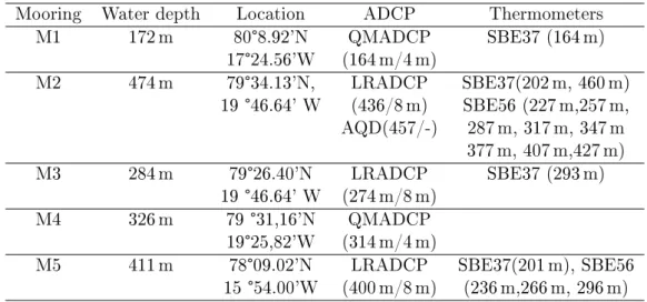
Table 2.1: Basic information on moorings M1-M5 Total water depth, coordinates, and attached instrument are provided for each mooring. For the attached ADPCs, the depth of the deepest measurement and the vertical resolution is stated, separated by "/". For the temperature measurements, the type of instrument and its depth is stated.

Mooring Water depth Location ADCP Thermometers

M1 172 m 80°8.92'N QMADCP SBE37 (164 m)

17°24.56'W (164 m/4 m)

M2 474 m 79°34.13'N, LRADCP SBE37(202 m, 460 m)

19 °46.64' W (436/8 m) SBE56 (227 m,257 m, AQD(457/-) 287 m, 317 m, 347 m

377 m, 407 m,427 m)

M3 284 m 79°26.40'N LRADCP SBE37 (293 m)

19 °46.64' W (274 m/8 m)

M4 326 m 79 °31,16'N QMADCP

19°25,82'W (314 m/4 m)

M5 411 m 78°09.02'N LRADCP SBE37(201 m), SBE56

15 °54.00'W (400 m/8 m) (236 m,266 m, 296 m) 2.1.3 Optimum Multiparameter Analysis

To characterize and distinguish mAIW at dierent locations, the relative contributions of the source water types that form mAIW were analyzed. An end-member analysis using the Optimum Multiparameter (OMP) approach as described below is used to achieve this goal. The following brief description of the OMP is based on previous work, provided to the reader in the appendix.

End-member water analysis is based on the idea of an unique set of water mass properties whose sinks and sources are only found at boundary interfaces (e.g. ocean/atmopshere, ocean/ice, Mackas et al., 1987). When transported away from the formation site, those properties do not change unless mixing occurs, where the conservative properties combine linearly to a new set of properties. This linearity allows to decompose a new water mass into its source water types by setting up a system of linear equations like the following:

d_obs,i= Σ x_iA_i+R_i (2.1)

In formula 2.1 each observed property of the water parcel d_obs is expressed as a linear combination of fractionsxi of the source-water masses and their characteristic properties A_i. Mass conservation is ensured by adding one equation that sums up all fractions to 1. In the case of an over-determined system (more properties than source water types), it can be solved by an Optimum Multiparameter Analysis (OMP, Hinrichsen and Tomczak, 1993; Huhn et al., 2008; Tomczak and Large, 1989).

In the ideal case, all observations can be fully explained by the linear equations and the residual R_i is zero. However, uncertainties in the measurements and/or the source water type denitions will lead to nonzero residuals. Therefore, a combination of positive mixing ratios is searched that minimizes the residual, i.e. the deviation between observed and computed properties (Huhn et al., 2008; Mackas et al., 1987). This is commonly done by nding the least squares solution of the problem in matrix formulation:

Ax−d_obs =R (2.2)

(18)

In this study, weighted linear equations are solved using the Matlab built in function lsqnonneg that solves constraint linear equation systems for both, the over-determined and the critical case. The calculated residuals of the equations are used as a measure of quality (Huhn et al., 2008).

The end-members of the AIW in 2016 and 2017 are found by picking the warmest and most saline measurements taken at the 79NG, i.e. the most outstanding peaks inΘ-S space. To account for variability, a mean of 12 peaks is used to dene the nal end-member (Huhn et al., 2008). The standard deviation expresses the error of the end-member denition.

Oxygen measurements corresponding to the points chosen in Θ-S space are averaged to dene the AIW oxygen end-member. A detailed explanation of the end-members of basal melt and runo which are found by theoretical considerations are explained in the appendix.

2.1.4 Wave speeds

Waves are present at a broad band of frequencies and speeds in the ocean, from high frequency internal waves to low frequency internal seiches. Waves originate when parcels are displaced by an external force in a medium which has a restoring force. The latter pushes the parcels back to its original position where it overshoots and is restored again (Talley et al., 2011).

The speed of waves depends on the type (i.e. the restoring force) and the properties of the medium (e.g. water depth, density). Here, two approximations described in Talley et al.

(2011) are stated that have been used in section 4.5.2 to estimate wave travel times. Surface gravity waves are induced by any forcing that mounds up or depresses the whole water column while gravity acts as restoring force. Shallow-water (long) gravity waves appear when the wavelengths are greater than the water depth H. Those waves are barotrop and non-dispersive, i.e. their phase speedc_p is constant and equal to the group speed that is given by:

c_p=p

gH (2.3)

Interfacial internal gravity waves describe an internal wave that is traveling along a density interface between two layers of dierent density within the stratied ocean. They are very similar to gravity waves and their speed is approximated using the reduced gravity (g') in equation 2.3.

c_p ≈ ∆ρ·g

ρ₀ H₁ =p

g⁰H₁ (2.4)

Here,ρ0 is the mean density of both layers, ∆ρ refers to the dierence in density between both layers and H1 is the mean thickness of the upper layer. This approximation is only valid when the upper layer is much thinner than the lower one. Internal waves have often much larger amplitudes than surface waves because the density contrast between the dierent water layers is strongly reduced in comparison to the density contrast between ocean and air. They are baroclinic, that implies for example that acceleration in the layers involved is directed to opposite directions.

(19)

2.2 Data sets related to atmosphere and cryosphere

2.2.1 Surface wind speeds over the Northeast Greenland continental shelf Wind observations were obtained from a weather station from the Danish Meteorological Institute on Henrik Kroeyer Holme, a group of islands located in Westwind Trough (80°38'N 13°43'W) about 90 km away from the mooring in Dijmphna Sund and about 170 km away from the main calving front. The data set consists of hourly wind speed and direction at 10 m above ground, together with a quality control ag. The time period between January 2015 and January 2018 was analyzed, but many missing information, particularly during the winter months, lead to the need of an additional data set.

Therefore, wind data from the Japanese 55-year Reanalysis (JRA-55) supported the analysis (Kobayashi et al., 2015). The data set has a resolution of approximately 55 km and contains among other variables wind speed at 10 m above the surface. Prior to the analysis of the wind eld described in section 3.3, all points covering the continental shelf were examined. Since there was little dierence in the general pattern, the wind information from the pixel, in which the mooring in Dijmphna Sund is located, was considered for further analysis only.

2.2.2 Sea ice concentration on the Northeast Greenland continental shelf Sea ice concentration data for the Northeast Greenland Shelf was downloaded from the University of Bremen that produces sea ice concentration maps based on the 89 GHz frequency of the Advanced Microwave Scanning Radiometer 2 (AMSR2) with a resolution of 3.125 km (AMSR2 Grosfeld et al., 2016; Spreen et al., 2008). This data set was chosen because due to its high spatial resolution it contained information on the sea ice conditions in the narrow (10 km wide ) Dijmphna Sund. Sea ice data was analyzed for September 2016 until March 2017 covering the same period as the current measurements do.

2.2.3 Basal melt rate estimates using the uxgate approach

To investigate a potential inuence of freshwater supply from the 79NG on the fjord circulation, a uxgate approach was chosen to estimate the basal melt rate (section 4.5.1). The uxgate approach is based on estimating the dierence of ice transport passing through an upper and lower gate within a certain time and to attribute the dierence to basal melt.

Therefore, it requires (a) glacier speeds from 2016 and 2017, (b) the grounding line and calving front position, (c) glacier thickness at the uxgates, and (d) the surface mass balance for 2016 and 2017. In the following, the data sets (a)-(d) are described (see also Tab.

2.2). Second, a short review on the uxgate method is given, mainly based on Enderlin and Howat (2013).

(a) Glacier speeds for 2016 were calculated using feature tracking on a set of six cloud-free optical images from 2016/05/04 to 2016/09/03 taken by Landsat 8 (NASA). For details on the method, the reader is directed to Fahnestock et al. (2016) and for a recent application of feature tracking on glacier velocities to Messerli et al. (2014). To ensure similar viewpoint and illumination conditions to reduce the noise, only images from similar satellite paths were taken that were acquired temporally close (max. one month apart). Feature tracking measures displacements between unique features as e.g. crevasses or debris on two images separated in time and relates them to surface motion. The displacement is found by moving a search window (here approx. 2 km × 2 km, corresponding to four times the expected displacement) by steps of 240 m and calculating the cross-correlation between each patch of an image. The highest correlation was expected to correspond to the displacement that

(20)

was converted to velocity taking into account the time dierence between the images. By averaging the results of all ve image pairs, an average glacier speed with a resolution of 250 m was produced. The displacement measured on stationary features close to the glacier was used to quantify the error of the speed, resulting in±105 m yr⁻¹ (Bevan et al., 2012;

Messerli et al., 2014; Paul et al., 2017).

For 2017 glacier speeds, there was already a data set with very similar characteristics available from ESA (Greenland Ice Sheet CCI). The glacier surface velocities have been created from feature-tracking of optical Sentinel-2 data (horizontal resolution 12 m) acquired between 2017/06/25 and 2017/08/10. The resolution of the data product is 50 m.

An error estimate of±204 m was obtained by calculating the standard deviation of pixels over stable terrain (Paul et al., 2017).

(b) The current grounding line zone (from 2017/03/05) of the 79NG was also available from ESA (Greenland Ice Sheet CCI). Remote sensing observations cannot provide direct measurements of the grounding line, but InSAR (Interferometric Synthetic Aperture Radar) provided by the ERS-1/-2 SAR tandem mission and Sentinel-1 SAR is able to detect the tidal exure zone by identifying very small changes in surface elevation and movements.

The calving front was mapped for both years from optical images.

(c) The ice thickness at the grounding line and the claving front was extracted from Bed- Machine v3 Greenland (Morlighem et al., 2017) that is compiled from a NASA's Operation IceBridge overight in 2014 (Mouginot et al., 2015, , supplement). The uncertainty is provided in the data set with± 20 m. The ice thickness data were compared at the calving front with the freeboard of the oating tongue in 2013-2015 taken from the ArcticDEM (Polar Geospatial Centre), a high-resolution digital elevation model (5 m resolution). Es- timating the total thickness of the oating ice tongue with a mean density of 970 kg m⁻³ of the glacial tongue indicated similar results as the one from BedMachine.

(d) Monthly surface mass balance data for 2016 and 2017 were obtained from B. Noël (personal communication, 2018). The data set is created by downscaling a RACMO2.3p2 run at 5.5 km resolution to 1 km resolution. The physics of the RACMO2.3p2 model are described in Noël et al. (2018).

Based on the grounding line and the calving front the uxgates were dened. The rst uxgate was set at the location of the grounding line. The second uxgate is located 15 km upstream of the calving front, before the 79NG splits into the main calving front and the minor calving front towards Dijmphna Sund. Since Wilson et al. (2017) showed that basal melting is negligible close to the calving front, the associated error was expected to be small.

To calculate basal melt rates, the steps that are explained in the following, are conducted (Enderlin and Howat, 2013):

1. Calculate discharge at both uxgates, one located at the grounding line and one close to calving front (equation 2.5).

2. Estimate thinning due to divergence using the glacier geometry (equation: 2.6).

3. Take the dierence between both uxgates, correct for the divergence and add the surface mass balance to obtain the basal melt rate (equation 2.7).

1. Discharge was calculated at the grounding line (subscript g) and at the calving front uxgate (subscriptf) using velocity (u), ice thickness (h) and glacier width (w) using the following equation:

Q=u·h·w (2.5)

(21)

Table 2.2: Overview of glacial data sets used for basal melt rate estimates

type of

dataset creator (ref-

erence) reference

date resolution additional information grounding

line ESA

Glacier CCI

March 2017 used for 2016 and 2017, constructed from InSAR ERS-1/- 2 and Sentinel-1

glacier velocities 2016

this study April to

Sept. 2016 240 m based on optical feature tracking

glacier velocities 2017

ESA Glacier CCI

June to Au-

gust 2017 50 m based on optical feature tracking

ice thick-

ness BedMachine

Greenland (Morlighem et al., 2017;

Mouginot et al., 2015)

2014 150 m mass conservation over

grounded ice and airborne gravity inversion over the oating ice tongue (Mouginot et al., 2015). Freeboard estimates of glacier tongue from ArcticDEM (Polar Geospatial Centre)

SMB B. Noël monthly,

2016-2017 1 km reanalyse data using RAM- CMO2.3p2 (Noël et al., 2018) 2. Divergence (Divwas calculated following Enderlin and Howat (2013) based on the speed gradient ^U^g^−U_L ^f, the width gradient ^W^g^−W_L ^f, the mean ice thicknessHmean= ^H^g^+H₂ ^f, and the mean glacier widthWmean= ^W^g^+W₂ ^f. L is referring to the length of the glacier along the main ow line. Consequently, divergence is given by:

Div=H_mean·U_g−U_f

L ·W_g−W_f

L ·W_mean·L (2.6)

3. The surface mass balance (SM B) reects an average at both uxgate locations. Finally, the basal melt rate was calculated by

mbasal= Q_g−Q_f +Div

Wmean·L +SM B (2.7)

Here,m_basal refers to an average of the whole oating ice tongue per year.

2.3 Time series analysis

A basic purpose of time series analysis is to dene the variability of a data series. Often, a signal consists of periodic and aperiodic components that are superimposed on a secular (long-term) trend and biased by uncorrelated random noise (?). To dierentiate those components, various tools are available that are described below, mainly based on ? and lecture material from Lilly (2017a).

The framework of the time series analysis is given by some general considerations. The fundamental frequency f₁ is the lowest frequency (longest period) that can be resolved, i.e., it describes a signal with a period equal to the total length of the recordT:

f1 = 1 N∆t = 1

T (2.8)

(22)

N refers to the number of measurements and ∆tto the time between two measurements.

The record length also determines the frequency resolution, i.e. how much two signals with frequenciesf₁ and f₂ must dier to be detectable that equals the fundamental frequency

δf =|f₂−f1|= 1 N∆t = 1

T (2.9)

The upper limit of the resolved spectra is given by the Nyquist frequency that is dened as

f_N = 1

2∆t (2.10)

and states that it takes at least two sampling intervals (i.e. three data points) to resolve a sinusoidal signal with frequencyfN. In practical applications, noise and measurement errors may increase this theoretical limit to rather four or more data points. Energy from frequencies unresolved by the sampling (too low or too high), is redistributed to the resolved frequencies and may cause errors, called aliasing.

Prior to many calculations, the data sets were interpolated linearly and ltered using the jlab toolbox by J. Lilly (Lilly, 2017b) and the Matlab built-in functions butter and ltlt.

The low-pass lters were constructed using a Hanning-lter. Since the start and end of the ltered time series is contaminated by edge-eects, those points are often lost. To avoid such a reduction, the time series is mirrored at the edge. Nevertheless, one needs to consider this fact when interpreting the end points. The band-pass lters were constructed as butter-worth lters of fourth order that have been proved before to be the most stable for the data used. They were applied with a function that performs zero-phase ltering that is achieved by ltering in both directions to avoid frequency dependend shifts of the signal (Matlab function ltlt).

Cross-covariance functions characterize the linear dependence of two time series (x, y) and were used to calculate correlation coecients for dierent time lags k. The normalized cross-covariance functionρx,y is dened by:

Cx,y(k∆t) = 1 N−1

N−k

X

1

[yi−y][x¯ _i+k−x]¯ (2.11) ρ_x,y = C_x,y(k∆t)

σxσy (2.12)

whereσrefers to the variance of the time series. The value of the cross-covariance function C at lag 0 was given as a measure of correlation (correlation coecient, ?, p.374-376).

Spectral estimates

Time series analysis can be done in time and in frequency domain. To transform a time series into the frequency domain, the Fourier transformation can be used. This method is based on the principle that one can decomposed a stationary time series into a linear combination of sines and cosines, called a Fourier series. For a discrete time seriesy(t) of nite lengthN, the Fourier series has the form

y(t_n) = 1 2A₀+

N/2

X

p=1

[A_pcos(2πf_pt) +B_psin(2πf_pt)] (2.13) wherefp are multiples of the fundamental frequency and n refers to dierent time steps t_n =t₁, t₂, ..., t_N =n·∆t. Important requirement for the functions used is that they are

(23)

independent from each other, i.e. the coecients can be determined independently and that a nite number of Fourier coecients will result in the minimum mean square error between the original data and the tted Fourier combination. The contributions of each function with frequency fp are weighted by the constant Fourier coecients Ap, Bp that describe the relative contribution of this frequency to the observed signal. This concept is used when estimating the power spectrum of a time series that displays the energy per unit frequency bandwidth for each frequency. The coecientsAp andBp are obtained by multiplying the Fourier series bycos(fpt) and sin(fpt), respectively and sum them up.

Ap = 2 N

N

X

n=1

yncos(2πpn

N ) (2.14)

A₀ = 2 N

N

X

n=1

y_n (2.15)

B_p = 2 N

N

X

n=1

y_nsin(2πpn

N ) (2.16)

B0 = 0 (2.17)

The squared amplitudes of the coecientsA_pandB_prefer to the variance of the frequency band and is called spectral energy.

The considerations mode above can be expanded to vector properties, e.g., velocity that is expressed as complex value.

w(t) =u(t) +iv(t) (2.18)

When calculating the spectrum of the complex-valued velocity, it is possible to split the spectra in au andv component, or in positive and negative parts, related to an clockwise and counterclockwise sense of rotation of the circular components. In the second case, the spectrum is called rotary spectrum. The current vectorw(t) can be expressed as Fourier series (here of innite length:)

w(t) = ¯u(t) +iv(t) +¯

∞

X

p=1

{e⁽

+p+− p)

2 [A⁺_p +A⁻_p] cos(w_pt+i(⁺_p +⁻_p)

2 ) (2.19)

+i(A⁺_p −A⁻_p) sin(wpt+(⁺_p +⁻_p)

2 )} (2.20)

where A⁺_p and A⁻_p reect the amplitudes of the rotary components and ⁺_p and ⁻_p the corresponding phase angles.

The result of Fourier analysis on a discrete time series is a periodogram spectral estimate.

This estimate diers from the true spectrum because of the nite length of the time series.

It can be considered as the product of an innitely long time series with a rectangular window, that is zero outside of the sampled time, and one during the sampled time. When transforming this product, the resulting spectrum is distorted by the rectangle function.

Therefore, when using the direct periodiogram method to calculate the Fourier coecients, a form of ltering is required to reduce the edge-eects. This is archived by using the Multi- taper method, that smooths the undesirable eects of the rectangle function. Additionally, the multiplication with the set of orthogonal functions (tapers) leads to frequency-domain averaging that increases the statistical reliability of the spectrum.

The resulting periodogram spectral estimate of the rotary components is normalized such that the sum of the negative (SN N) and the positive (SP P) component approximates the

(24)

variance of the time series of length N. Consequently, the variance of the time series is then equal to

σ_odd² = 1

2π ·(f₂−f₁)·(

N

X

2

SPP+

N

X

2

SNN) (2.21)

σ²_even= 1

2π ·(f2−f1)·(

N−1

X

2

SPP+

N−1

X

2

SNN) (2.22)

In case N is even (σ²_even), the calculation is adapted (as shown) to avoid the duplication of the Nyquist frequency (Lilly, 2017a). In this study, variance is used as measure of variability. For a discrete time series y of length N with the mean y¯, an estimate of the variance is given by:

σ² ≡= 1 N

N

X

i=1

[yi−y]¯² (2.23)

When variance is quantied in this study in respect to dierent frequency ranges, it was calculated integrating the spectral estimate as expressed in equation 2.22 over a certain frequency range. Figure 3.6 illustrates the areas that have been integrated. The spectral estimates have been calculated with a Matlab routine provided by J. Lilly that calculates multi-taper spectra (Lilly, 2017b).

Harmonic Analysis

While Fourier analysis can only t amplitudes to multiples of the fundamental frequency, harmonic analysis provides another approach to determine the relative importance of well- known frequencies. Here, it is used to t functions at tidal frequencies to the discrete time series. Since there are more observations than functions of interest, this leads to an overdetermined problem which is solved by using optimization techniques. That implies to minimize the squared dierence between the original data and the t of the time series as it is implemented in the Matlab package t-tide (see Pawlowicz et al., 2002, for details).

Wavelets

When the amplitudes of the dierent functions of the Fourier analysis vary in time, the basic assumption of the Fourier analysis is violated. In such cases of non-stationary time series, wavelet transforms are more suited because they "unwrap" the spectrum across time. A wavelet is an oscillating function that is localized in time. For instance, the Morlet wavelet, that is the product of a complex exponential function, that controls the oscillation, multiplied by a Gaussian that leads to the localization in time. Calculating a wavelet transform means comparing the variability of the original time series with the known variability of the mother wavelet. This mother wavelet can be trimmed to have varying degrees of oscillation at each time step of the time series. In this way, the mother wavelet can be used to estimate the variability at each time step. Hereby, resolution in time and frequency still obey the Heisenberg uncertainty relation ∆t∆f < ¹₄π, i.e., increasing the temporal resolution decreases the frequency resolution and vice versa. Here, general- ized morse wavelets were calculated and applied on the time series, using the functions provided by the toolbox of J. Lilly (Lilly, 2017b). The morse wavelets are controlled by two parameters. One characterizes the symmetry of the wavelets in the frequency domain.

The other one describes the bandwidth of the frequency domain. Increasing this parame- ter leads to highly time-localized as opposed to frequency-localized wavelets. Plotting the

(25)

averaged amplitude of each frequency at each time step leads to a wavelet plot as e.g. 4.5.

For details on morse wavelets and the mathematical expressions of wavelts in general see also Lilly and Olhede (2012).

Empirical Orthogonal Functions

Empirical orthogonal function analysis (EOFs, also known as principal component analysis) is an inverse technique that decomposes a signalΨinto a linear combination of orthogonal functionsφ(also called statistical "modes") scaled by an amplitudeα. This can be written as

Ψ(zm, t) =

M

X

i=1

αi(t)φi(m) (2.24)

with the orthogonality condition (δ_ij is Kronecker delta)

M

X

m=1

φ_i(m)φ_j(m) =δ_ij (2.25) EOFs have the advantage that variability, that is not coherent within the data set, is sup- pressed and connections between the records are emphasized. For a unique determination of the EOFs, the amplitudes are uncorrelated over the sample data. Prior to calculations, the time series is de-trended.

Usually, already the rst few functions account for most of the variance of the time series and their pattern may be, but does not have to be linked to a dynamical mechanism.

EOFs therefore provide a compact description of the spatial and temporal variability of a data series. Mathematically, the EOF analysis is equivalent to solving for eigenvectors (the EOFs) and corresponding eigenvalues (the amplitude) of a matrix. In matrix formulation this can be written as

CΦ−λIΦ= 0 (2.26)

whereC represents the covariance matrix, I is the unity matrix, λ the variance in each mode, andΦare the eigenvectors. Solving the eigenvalue problem includes transformation the system into a diagonal matrix that represents a set of orthogonal functions, the EOFs.

In the diagonal matrix, the EOFs are ordered by the variance that is associated with them, i.e. the rst mode contains the highest percentage of total variance. In total, the variance of the time series equals the sum of the variance in the eigenvalues. The modes reect a variation in both directions around the mean. Their amplitude (phase and magnitude) is determined by the time dependent amplitudes of the EOFs that are given by:

α_i(t) =

M

X

m=1

Ψ_m(t)Φ(m)_i (2.27)

An example of EOFs and their amplitudes are displayed in Fig. 4.7.