Bayesian Analysis of Network Data  Model Selection and Evaluation of the Exponential Random Graph Model

Model Selection and Evaluation of the Exponential Random Graph Model

Dissertation

Presented to the Faculty for

Social Sciences, Economics, and Business Administration at the

Otto-Friedrich-University of Bamberg

in Partial Fulllment of the Requirements for the Degree of DOCTOR RERUM POLITICARUM

Julian Körber, Master of Science in Survey Statistics by born July 3, 1984 in Forchheim, Germany

Bamberg

2018

Principal advisor: Professor Dr. Susanne Rässler University of Bamberg, Germany Reviewers: Professor Dr. Kai Fischbach

University of Bamberg, Germany Professor Dr. Lasse Gerrits

University of Bamberg, Germany Date of submission: November 27, 2017

Date of defence: March 29, 2018

URN: urn:nbn:de:bvb:473-opus4-516206

DOI: https://doi.org/10.20378/irbo-51620

The exponential random graph model (ERGM) is a class of stochastic models for network data widely applied in statistical social network analysis. The ERGM can be used to model a wide range of social processes. However, it is generally dicult to estimate due to its intractable normalizing constant. Markov chain Monte Carlo maximum likelihood (MCMC-ML) ERGM estimation is available but tends to be numerically unstable due to model degeneracy of particular specications. Bayesian ERGM estimation is robust to model degeneracy and is a practical alternative to the MCMC-ML approach.

Bayesian model selection is based on the Bayes factor which is the ratio of marginal likelihoods of concurring models. The research aim of this thesis is to estimate the marginal likelihood of the ERGM class using path sampling which is also called thermodynamic integration. Power posterior sampling is a discreti- zed version of thermodynamic integration using a xed path of tempering steps to transition from the prior distribution to the posterior distribution of interest. In this thesis, power posterior sampling is used both to integrate over the parameter space of the ERGM posterior distribution of interest and to yield an estimate of the respective intractable ERGM normalizing constant. Existing approaches of estimating the ERGM marginal likelihood rely on a non-parametric density ap- proximation or a Laplace approximation. The proposed power posterior exchange algorithm with explicit evaluation of the likelihood (PPEA-EEL) does not require such approximations and yields a valid estimate of the ERGM marginal likeli- hood. As the PPEA-EEL is a computationally expensive approach involving many MCMC samples, new graphical methods to evaluate power posterior samples are developed.

In this thesis a brief introduction to random graphs and network dependencies

is given. The ERGM class is discussed and various dependency assumptions are

illustrated. MCMC-ML ERGM estimation is applied to policy networks in Ghana,

Senegal and Uganda. Bayesian ERGM estimation and Bayesian model selection are

discussed. An overview is given on methods of estimating the marginal likelihood

originating from importance sampling, namely bridge sampling, path sampling and

power posterior sampling. The PPEA-EEL is applied to social network data and

the numerical stability of the approach is evaluated.

Contents

List of Tables XI

List of Figures XIII

1 Introduction 1

1.1 Exponential random graph models . . . . 2

1.2 Bayesian model selection . . . . 3

1.3 Problems and research aims . . . . 4

1.4 Overview . . . . 6

2 Exponential random graph models 9 2.1 Networks as random graphs . . . . 10

2.2 Network statistics . . . . 12

2.3 Model denition and interpretation . . . . 17

2.3.1 Dependence graphs and sucient statistics . . . . 19

2.3.2 Log-linear formulation . . . . 22

2.4 Dependence assumptions . . . . 24

2.4.1 The Bernoulli random graph model . . . . 24

2.4.2 The dyad independence model . . . . 27

2.4.3 The Markov model . . . . 29

2.4.4 The social circuit model . . . . 30

2.4.5 Including exogenous covariates . . . . 33

2.5 Maximum likelihood estimation and network simulation . . . . 35

2.5.1 Simulating Networks . . . . 35

2.5.2 Markov chain Monte Carlo maximum likelihood estimation 41 2.5.3 Goodness of t evaluation . . . . 45

2.5.4 Model degeneracy . . . . 46

VII

2.6 Extensions and modeling alternatives . . . . 50

3 Determinants of communication in policy networks in Ghana, Se- negal and Uganda 53 3.1 Introduction . . . . 53

3.2 Determinants of communication in policy networks . . . . 56

3.3 Survey design and statistical framework . . . . 60

3.4 Empirical analysis . . . . 68

3.5 Conclusion . . . . 72

4 Bayesian exponential random graph model estimation 75 4.1 Bayesian inference . . . . 76

4.2 The exchange algorithm . . . . 77

4.3 Adaptive direction sampling . . . . 80

4.4 Application . . . . 82

4.4.1 Krackhardt's Managers . . . . 82

4.4.2 Expert network in Ghana . . . . 89

4.5 Summary . . . . 91

5 Bayesian model selection for network data 93 5.1 The Bayes factor . . . . 95

5.2 Computing the model evidence . . . . 98

5.2.1 Importance sampling . . . . 98

5.2.2 Bridge sampling . . . 100

5.2.3 Path sampling . . . 102

5.2.4 Power posterior sampling . . . 106

5.2.5 Other approaches . . . 109

5.3 The power posterior exchange algorithm . . . 111

5.3.1 Power posterior step . . . 111

5.3.2 Explicit evaluation of the intractable likelihood . . . 114

5.4 Application . . . 116

5.4.1 Krackhardt's managers . . . 117

5.4.2 The PEBAP expert network in Ghana . . . 133

5.5 Summary . . . 137

6 Summary and discussion 141

6.1 Limitations and alternatives . . . 143

6.2 Outlook . . . 144

A Exponential random graph models 147 A.1 The Bernoulli random graph model is an ERGM . . . 147

A.2 Tables . . . 150

A.3 Figures . . . 152

B Determinants of communication in policy networks 155 B.1 Survey questions . . . 155

B.2 Tables . . . 157

B.3 Figures . . . 161

C Bayesian exponential random graph model estimation 165 C.1 Krackhardt's managers . . . 166

C.2 Ghana . . . 169

D Bayesian model selection for network data 177 D.1 The path sampling identity . . . 177

D.2 Power posterior sampling . . . 179

D.3 PPEA Krackhardt's managers . . . 180

D.4 PPEA Ghana . . . 186

D.4.1 Model 1 . . . 186

D.4.2 Model 2 . . . 192

D.4.3 Model 3 . . . 198

D.4.4 Model 4 . . . 204

D.4.5 Model 5 . . . 210

D.4.6 Model 6 . . . 216

List of Tables

2.1 Simulated toy networks: Exogenous covariates of simulated networks 37 2.2 Simulated toy networks: Parameter specications used for network

simulation . . . . 38 4.1 Krackhardt's managers: EA parameter estimates . . . . 87 4.2 Expert network Ghana: EA parameter estimates . . . . 90 5.1 Interpretation of the Bayes factor according to Kass and Raftery

(1995) . . . . 96 5.2 Krackhardt's managers: PPEA-EEL results . . . 133 5.3 Expert network Ghana: PPEA-EEL results . . . 135 A.1 Simulated toy networks: Summary of sucient network statistics,

specication 1 . . . 150 A.2 Simulated toy networks: Summary of sucient network statistics,

specication 2 . . . 151 B.1 Classication of actors with absolute and relative frequency . . . . 157 B.2 Model terms and aliated hypotheses . . . 158 B.3 ERGM parameter estimates all countries . . . 159

XI

List of Figures

2.1 Transitive and intransitive triads . . . . 16

2.2 Examples of common directed network statistics . . . . 17

2.3 Dependence graphs resulting from dierent assumptions of conditi- onal independence . . . . 21

2.4 Change in network statistic counts . . . . 23

2.5 2 -triangle as 4 -cycle . . . . 31

2.6 Simulated toy networks: GOF plots, specication 1 . . . . 40

2.7 Simulated toy networks: GOF plots, specication 2 . . . . 40

2.8 Two typical simulated toy networks . . . . 41

2.9 Illustration of strong degeneracy . . . . 49

2.10 Illustration of weak degeneracy . . . . 49

3.1 Plot: Ghana expert network . . . . 65

3.2 Plot: Ghana support network . . . . 66

3.3 Plot: Senegal expert network . . . . 66

3.4 Plot: Senegal support network . . . . 67

3.5 Plot: Uganda expert network . . . . 67

3.6 Plot: Uganda support network . . . . 68

4.1 Plot: Krackhardt's friendship network . . . . 83

4.2 Absence of degeneracy for Krackardt's network . . . . 83

4.3 Krackhardt's network: EA Traceplots, model 2 . . . . 85

4.4 Krackhardt's network: ACF of EA chains, model 2 . . . . 86

4.5 Krackhardt's network: Densities of merged EA sample, model 2 . . 86

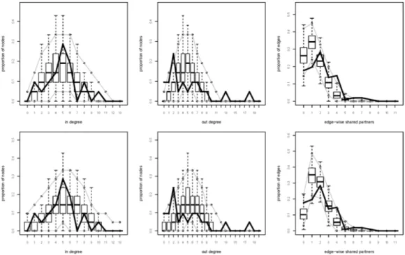
4.6 Krackhardt's network: GOF EA, model 1 and model 2 . . . . 88

4.7 Expert network Ghana: GOF EA, model 1 . . . . 91

XIII

4.8 Expert network Ghana: GOF EA, model 2 . . . . 91

5.1 Power posterior temperature schedule . . . 118

5.2 PPEA Krackhardt's managers, model 2: Traceplots . . . 120

5.3 PPEA Krackhardt's managers, model 2: Density plots . . . 121

5.4 PPEA Krackhardt's managers, model 2: Mean retries per accepted draw . . . 122

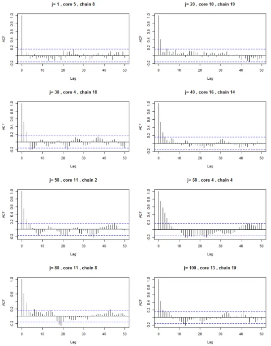
5.5 PPEA Krackhardt's managers, model 2: Sample of ACF plots . . . 123

5.6 PPEA Krackhardt's managers, model 2: Summary of MCMC auto- correlation . . . 124

5.7 PPEA Krackhardt's managers, model 2: ACF plots of merged chains 125 5.8 PPEA Krackhardt's managers, model 2: ACF plots of thinned mer- ged chains . . . 126

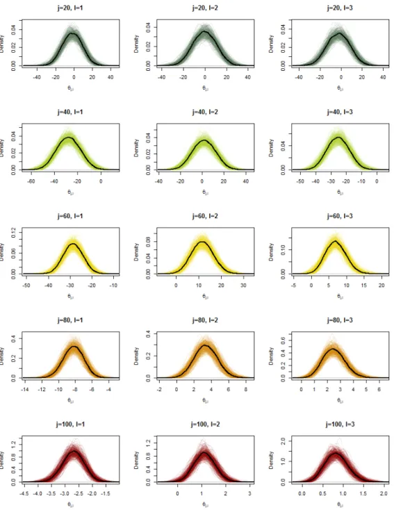
5.9 PPEA Krackhardt's managers, model 2: Densities of the edge para- meter over temperatures . . . 127

5.10 PPEA Krackhardt's managers, model 2: MCMC estimates of θ

. 128 5.11 PPEA Krackhardt's managers, model 2: MCMC estimates of θ

multiplied by t . . . 128

5.12 PPEA Krackhardt's managers, model 2: MCMC estimates of θ

over t . . . 129

5.13 PPEA Krackhardt's managers, model 2: MCMC estimates of θ

multiplied by t

over temperature . . . 129

5.14 PPEA-EEL Krackhardt's managers, model 2: Tempered likelihood 131 5.15 PPEA-EEL Krackhardt's managers, model 2: Marginal likelihood . 132 5.16 PPEA-EEL Ghana, model 2: Normalizing constants of the tempered likelihoods . . . 136

5.17 PPEA-EEL Ghana, model 2: Estimate of the evidence, additional importance draws . . . 137

A.1 Simulated toy networks: Summary of sucient statistics, specica- tion 1 . . . 152

A.2 Simulated toy networks: Summary of sucient statistics, specica- tion 2 . . . 153

B.1 Goodness-of-t Ghana Expert network: Model 1 and model 2 . . . 161

B.2 Goodness-of-t Ghana Expert network: Model 3 and model 4 . . . 161

B.3 Goodness-of-t Senegal Expert network: Model 1 and model 2 . . . 162

B.4 Goodness-of-t Senegal Support network: Model 3 and model 4 . . 162

B.5 Goodness-of-t Uganda Expert network: Model 1 and model 2 . . 163

B.6 Goodness-of-t Uganda Support network: Model 1 and model 2 . . 163

C.1 Krackhardt's managers: EA Traceplots, model 1 . . . 166

C.2 Krackhardt's managers: ACF of EA chains, model 1 . . . 167

C.3 Krackhardt's managers: Densities of merged EA sample, model 1 . 168 C.4 Ghana: EA Traceplots, model 1 . . . 169

C.5 Ghana: ACF of EA chains, model 1 . . . 170

C.6 Ghana: Densities of merged EA sample, model 1 . . . 171

C.7 Ghana: EA Traceplots, model 2 . . . 172

C.8 Ghana: ACF of EA chains, model 2 . . . 173

C.9 Ghana: Densities of merged EA sample, model 2 . . . 174

C.10 Ghana: Check for degeneracy, model 1 and model 2 . . . 175

D.1 PPEA Krackhardt's managers, model 1: Traceplots . . . 180

D.2 PPEA Krackhardt's managers, model 1: Density plots . . . 181

D.3 PPEA Krackhardt's managers, model 1: Summary of MCMC auto- correlation . . . 182

D.4 PPEA Krackhardt's managers, model 1: MCMC estimates of θ

. 183 D.5 PPEA Krackhardt's managers, model 1: Tempered likelihood . . . 184

D.6 PPEA Krackhardt's managers, model 1: Marginal likelihood . . . . 185

D.7 PPEA Ghana, model 1: Traceplots . . . 186

D.8 PPEA Ghana, model 1: Density plots . . . 187

D.9 PPEA Ghana, model 1: Summary of MCMC autocorrelation . . . 188

D.10 PPEA Ghana, model 1: MCMC estimates of θ

. . . 189

D.11 PPEA Ghana, model 1: Tempered likelihood . . . 190

D.12 PPEA Ghana, model 1: Marginal likelihood . . . 191

D.13 PPEA Ghana, model 2: Traceplots . . . 192

D.14 PPEA Ghana, model 2: Density plots . . . 193

D.15 PPEA Ghana, model 2: Summary of MCMC autocorrelation . . . 194

D.16 PPEA Ghana, model 2: MCMC estimates of θ

. . . 195

D.17 PPEA Ghana, model 2: Tempered likelihood . . . 196

D.18 PPEA Ghana, model 2: Marginal likelihood . . . 197

D.19 PPEA Ghana, model 3: Traceplots . . . 198

D.20 PPEA Ghana, model 3: Density plots . . . 199

D.21 PPEA Ghana, model 3: Summary of MCMC autocorrelation . . . 200

D.22 PPEA Ghana, model 3: MCMC estimates of θ

. . . 201

D.23 PPEA Ghana, model 3: Tempered likelihood . . . 202

D.24 PPEA Ghana, model 3: Marginal likelihood . . . 203

D.25 PPEA Ghana, model 4: Traceplots . . . 204

D.26 PPEA Ghana, model 4: Density plots . . . 205

D.27 PPEA Ghana, model 4: Summary of MCMC autocorrelation . . . 206

D.28 PPEA Ghana, model 4: MCMC estimates of θ

. . . 207

D.29 PPEA Ghana, model 4: Tempered likelihood . . . 208

D.30 PPEA Ghana, model 4: Marginal likelihood . . . 209

D.31 PPEA Ghana, model 5: Traceplots . . . 210

D.32 PPEA Ghana, model 5: Density plots . . . 211

D.33 PPEA Ghana, model 5: Summary of MCMC autocorrelation . . . 212

D.34 PPEA Ghana, model 5: MCMC estimates of θ

. . . 213

D.35 PPEA Ghana, model 5: Tempered likelihood . . . 214

D.36 PPEA Ghana, model 5: Marginal likelihood . . . 215

D.37 PPEA Ghana, model 6: Traceplots . . . 216

D.38 PPEA Ghana, model 6: Density plots . . . 217

D.39 PPEA Ghana, model 6: Summary of MCMC autocorrelation . . . 218

D.40 PPEA Ghana, model 6: MCMC estimates of θ

. . . 219

D.41 PPEA Ghana, model 6: Tempered likelihood . . . 220

D.42 PPEA Ghana, model 6: Marginal likelihood . . . 221

Chapter 1 Introduction

Networks represent relations between entities. These entities are called nodes and the relations are called edges. Depending on the type of nodes and the type of ed- ges considered, a variety of networks can be dened. Social networks indicate the relations between social actors and represent social processes. Such social processes are e.g. the communication of political actors, relations within an organization or friendship within a class room. This thesis is restricted to human social networks where social actors are human individuals or collectives of individuals like organiza- tions. Social processes typically generate patterns like reciprocity, transitivity and hierarchy which are not easy to model statistically. Stochastic models for network data have to capture such patterns of tie variable formation while recognizing the variability that cannot be modeled explicitly. Most stochastic models rely on the assumption of independent and identically distributed observations which would risk incorrect inference in network analysis, while stochastic models for network data explicitly try to formulate the dependence between social actors and network ties. Wasserman and Faust (1994) and Jackson (2008) give a general introduction to statistical social network analysis. Kolaczyk (2009) and Snijders (2011) give an overview on stochastic models for network data.

The exponential random graph model (ERGM) is a class of stochastic models for binary network ties as dependent variables and is by far the most widely used model for statistical social network analysis. It can model a wide range of hypothe- sized patterns of network tie formation originating from many strands of theories.

Network ties can be modeled conditional on endogenous patterns of network self organization and exogenous covariates based on actor attributes which allows for a

1

high exibility in social network analysis. The ERGM class can also be applied to networks where the nodes are non-human entities, e.g. technological or biological networks.

1.1 Exponential random graph models

An observed binary network is considered as the realization of a random graph.

A random graph is a collection of random binary tie variables on a xed set of nodes. If all tie variables are assumed to be independent, network tie formation can be modeled with a Bernoulli process. However, this would be a very unrealistic data generating mechanism in most cases, therefore stochastic models are required which can capture realistic patterns of network tie formation. The ERGM class can be used to explicitly model patterns of network dependence such as endoge- nous network self organization and the inuence of exogenous nodal attributes.

Patterns of tie formation are represented by fundamental subgraph congurations like triangles or stars and congurations depending on nodal attributes. Counts of such congurations are used as sucient statistics for the ERGM probability distribution. While the ERGM is not a new model class at all, it did not gain po- pularity in statistical social network analysis for a long time until severe problems of model estimation were solved.

The most simplistic Bernoulli random graph model dates back to Erdös and Renyi (1959). Besag (1974) show how a random graph model can be formulated in an exponential form using counts of subgraph congurations as sucient statistics.

Holland and Leinhardt (1981) develop the rst ERGM specication that is able to

represent patterns of reciprocity. The Markov model by Frank and Strauss (1986)

is able to capture patterns of transitivity, hierarchy and centrality. The Markov

model was a break trough in statistical social network analysis. However, it is very

hard to estimate, which prevented its application for two decades. Wasserman and

Pattison (1996) introduce a log-linear formulation of the ERGM which facilitates

the interpretation and allows for the inclusion of exogenous covariates. A more

general dependence assumption formulated by Pattison and Robins (2002) and

implemented by Snijders et al. (2006) generated a break through for the ERGM

class. Hunter and Handcock (2006) develop Markov Chain Monte Carlo maximum

likelihood (MCMC-ML) ERGM estimation based on simulated networks. Bayesian

ERGM estimation is introduced by Koskinen (2008) and Caimo and Friel (2011).

The major drawback of the ERGM class is the diculty of model estimation which is caused by model degeneracy and the unavailability of the likelihood nor- malizing constant. The latter requires auxiliary network simulations and renders methods of model estimation computationally expensive. The rst can cause con- vergence issues as it may be impossible to nd suitable starting values for the MCMC-ML approach. Bayesian ERGM estimation using the exchange algorithm (EA) by Murray et al. (2006) is robust to model degeneracy. Today, the ERGM class is widely applied and many extensions are available, see the Lusher et al., eds (2012) for an overview.

1.2 Bayesian model selection

In Bayesian statistics the prior distribution p(θ) represents the assumptions about the population characteristics before data are observed. The likelihood function p(y|θ) represents the data generating process and the posterior distribution

p(θ|y) = p(θ)p(y|θ)

p(y) (1.1)

represents the updated assumptions if data are observed. The normalizing constant p(y) is called the marginal likelihood. In most cases the analytical evaluation of the posterior distribution is not possible and MCMC techniques are required.

The Bayesian approach allows for model comparison using the posterior odds of concurring models m

and m

Pr(m

|y)

Pr(m

|y) = Pr(m

)

Pr(m

) × p(y|m

)

p(y|m

) . (1.2)

The prior odds Pr(m

)/ Pr(m

) are updated with the Bayes factor p(y|m

)/p(y|m

) which is a ratio of marginal likelihoods. The marginal likelihood is the normalizing constant of the respective posterior distribution. Typically, the prior odds are assumed to be one so the Bayes factor is the relevant quantity for model comparison.

In this role the marginal likelihood is also called the model evidence. Computation

of the model evidence is a complicated task and requires techniques of numerical

integration for most cases.

Importance sampling can be used to estimate the model evidence, see Ge- weke (1989), although it may be very dicult to specify an ecient importance function. Bridge sampling introduced by Meng and Wong (1996) estimates the ratio of normalizing constants using importance samples from two non-normalized distributions. If a bridging distribution with known normalizing constant is used, this approach can be applied to estimate the evidence of the target distribution.

If the Kullback-Leibler divergence (Kullback, 1968) between the target distribu- tion and the bridging distribution is too large, bridge sampling will be inecient.

Gelman and Meng (1998) introduce path sampling which uses an innite number of bridging distributions in order to estimate the ratio of normalizing constants.

In statistical physics this approach is also called thermodynamic integration, see Ogata (1989), where integration over a parameter space is achieved by transiting over a temperature range. In Bayesian statistics this corresponds to a transition from the prior distribution to the posterior distribution of interest. Power posterior sampling, which is a discretized version of path sampling, uses a xed number of temperature steps transiting from the prior to the posterior, see Friel and Pettitt (2008). A class of tempered posterior distributions is constructed which can be used to integrate over the parameter space of the posterior of interest. MCMC simulations from the tempered posteriors yield an estimate of the evidence using a trapezoidal approximation. If the discretized temperature path is well chosen and a suciently large number of temperature steps is used, the Kullback-Leibler divergence between subsequent tempered posteriors will be small. This results in a low discretizational error in the trapezoidal approximation. The estimation of the ERGM evidence is especially challenging as the normalizing constant of the likelihood is not available. Path sampling can be used to yield an estimate of this normalizing constant, see Hunter and Handcock (2006) and Friel (2013).

1.3 Problems and research aims

The MCMC ML approach introduced by Hunter and Handcock (2006) is a popular

method for ERGM estimation. However, it can be numerically very unstable and

nding suitable starting values can be dicult due to model degeneracy. A Baye-

sian approach introduced by Caimo and Friel (2011) is robust to model degeneracy

and is a practical alternative for ERGM estimation. The Bayes factor can be used

for ERGM selection which requires estimation of the model evidence.

The main research aim for this thesis is to yield a valid estimate of the ERGM evidence using power posterior sampling. This approach requires MCMC simula- tion from tempered posterior distributions and evaluation of the intractable ERGM likelihood. A combination of the EA and power posterior sampling is proposed which will be referred to as power posterior exchange algorithm (PPEA). The normalizing constant of the ERGM likelihood is estimated using the identity in- troduced by Meng and Wong (1996) which allows for the explicit evaluation the likelihood (EEL) of the intractable ERGM class. The EEL can be achieved as a byproduct of power posterior sampling as it uses the same discretized temperature path to estimate the normalizing constant of the likelihood. This approach yields a valid estimate of the ERGM evidence and shall be referred to as power posterior exchange algorithm with explicit evaluation of the likelihood (PPEA-EEL).

Two other approaches of estimating the ERGM evidence are known. Similar to the PPEA-EEL, Caimo and Friel (2013) and Friel (2013) use path sampling to estimate the normalizing constant of the ERGM likelihood. The ERGM evidence is estimated using the identity introduced by Chib (1995) while the posterior is evaluated using a non-parametric density estimate of a MCMC sample simulated with the EA. This approach is restricted to ERGM specications with at most ve parameters. Thiemichen et al. (2016) apply a Laplace approximation to estimate the evidence of more complex ERGM specications. They also use path sampling to estimate the ERGM normalizing constant and apply a Laplace approximation to a MCMC sample. This approach requires the strong assumption that the pos- terior can be approximated by a normal distribution which in many cases will not hold. The PPEA-EEL requires no approximation assumptions of the posterior and can be used if a non-parametric kernel density estimate is not available. However, the PPEA-EEL is computationally very expensive and not easy to implement. It requires complicated specications and the evaluation of numerous MCMC simula- tions. At the end of this thesis, best practice recommendations for the PPEA-EEL specication are given.

The second research aim is to develop tools for the evaluation of power pos-

terior sampling algorithms. Graphical methods are developed that allow for the

inspection of the tempered posteriors transiting from the prior to the posterior. As

numerous MCMC chains have to be inspected, aggregating methods are proposed

which help to evaluate the convergence of the power posterior sampler. Further-

more, a method to evaluate the trapezoidal approximation is proposed which helps to judge the reliability of the PPEA-EEL. This methods suggests to adapt the im- portance sample size in the EEL-step to the step size of the discretized path which is a new insight in this eld of research.

1.4 Overview

In chapter 2, the notation for network data and random graphs used throughout this thesis is introduced. It is shown how network statistics can be used to describe observed networks. The ERGM class is introduced and various assumptions of network dependency are illustrated. Methods of network simulation are introduced and ERGM estimation using the MCMC-ML approach is discussed. Finally, model degeneracy is illustrated and an overview on ERGM extensions and alternative stochastic models for network data is given.

In chapter 3, MCMC-ML ERGM estimation is applied to policy networks in Ghana, Senegal and Uganda. The communication ties between relevant actors of policy formulation are modeled using network statistics derived from various theories on policy formation and political communication. While the ERGM class has been used to model policy networks in developed countries before, this approach is completely new to developing countries. The MCMC-ML method used in chapter 3 is plagued by model degeneracy which causes numerical instability.

Bayesian ERGM estimation using the EA is robust to model degeneracy. In chapter 4, the fundamentals of Bayesian statistics are discussed. The EA uses auxiliary data simulated from the non-normalized ERGM likelihood in order to circumvent the evaluation of its intractable normalizing constant. The EA is ap- plied to estimate ERGM specications for Krackhardt's friendship network, see Krackhardt (1987) and the expert network in Ghana.

In chapter 5, Bayesian model selection using the marginal likelihood is dis-

cussed. The focus is on methods descending from importance sampling which are

bridge sampling, path sampling and power posterior sampling. The PPEA is intro-

duced as a new method of power posterior sampling for the ERGM class using the

EA. It is shown how the temperature path constructed for the PPEA can be used

to estimate the normalizing constant of the ERGM likelihood which allows for the

EEL-step. The proposed new PPEA-EEL approach uses MCMC simulations from

the tempered posterior distributions and the corresponding sequence of explicitly evaluated tempered likelihood functions in order to yield an estimate of the ERGM evidence. The PPEA-EEL is applied to the Krackhardt's managers network and the expert network in Ghana. New graphical methods to evaluate the behaviour of the PPEA transiting over the temperature path are introduced.

Chapter 6 summarizes the thesis and discusses limitations of the PPEA-EEL

and alternatives to this approach. Finally, an outlook is given on future research

and how the eciency of the PPEA-EEL can be increased.

Chapter 2

Exponential random graph models

Statistical models for binary outcomes like the logistic regression approach rely on the assumption of independence of observations. When analyzing network data this assumption is unrealistic as it is well known that individual behaviour depends on the interaction with others. In the simplest case of tie variable interdependence the probability of a tie from alter to ego might depend on the existence of a tie from ego to alter. Further, it is well known that social interaction is often structu- red after the principle `a friend of a friend is a friend'. The process of network tie formation has to be modeled in such a way that observations are independent con- ditional on explicitly formulated features of dependency. The exponential random graph model (ERGM) popularized by Wasserman and Pattison (1996) solves this problem for binary network data.

The ERGM can be used to test for a lot of hypothesized patterns of network interdependence including the inuence of exo- genous covariates. However, as will be discussed in section 2.5, this potential is limited by the numerical eort required for parameter estimation.

In section 2.1 a notation for random graphs and network data is introduced and the description of networks using appropriate summary statistics is discussed. It is shown how binary network data can be understood statistically as realizations of a random graph. In section 2.3 the ERGM model class is dened. It is illustrated how a dependence graph is used to deduce aliated sucient network statistics.

1Wasserman and Pattison (1996) refer to the p^∗ model. This term is no longer in use in the literature.

9

Various dependence assumptions are discussed in section 2.4 which help to formu- late realistic models of network tie formation. Maximum likelihood (ML) ERGM estimation, which is introduced in section 2.5, requires Markov chain Monte Carlo (MCMC) methods of network simulation. MCMC-ML ERGM estimation which helps to circumvent the explicit evaluation of the intractable ERGM likelihood function is illustrated. The common problem of model degeneracy is discussed.

Finally, a short overview of ERGM extensions and modeling alternatives is given.

2.1 Networks as random graphs

In social network analysis the relations between a xed set of units (nodes) are con- sidered. Typically nodes are actors such as friends within a class room, employees within an organization, organizations within a political system or national states in the global context. The relational links between two nodes are called edges or ties. Throughout this work we consider only binary ties which may be present or absent but have no relational weight such as the relative importance of a friendship.

Consider a xed set of n nodes that may or may not be connected by a tie. The relation between the pair of nodes i and j may be indicated by a binary random tie variable

Y

= 1, i > j if the two nodes are connected and

Y

= 0, i > j

else. If Y

= 1 , an edge y

exists between the two nodes whereas self ties y

are

not allowed for any i. If directed relations are considered, the random tie variables

Y

6= Y

i.e. it is of concern which of the nodes is sending a tie towards the

other node. For undirected relations Y

= Y

. The collection of all N random

tie variables on a xed set of n nodes is called a random graph Y which may be

represented by a n × n random adjacency matrix. Throughout this work capital

letters denote random variables and small letters denote realizations: Y denotes

a random graph on n nodes, Y

denotes a random tie variable. y denotes an

observed network represented by an n × n adjacency matrix and y

denotes an

observed tie. The diagonal of the adjacency matrix y is always empty as self ties

are not allowed. An entry in row i and column j represents the observed tie variable y

. For undirected graphs the adjacency matrix y is symmetric. If directed graphs (digraphs) are considered the upper and the lower triangular matrices of y are distinct. For undirected graphs the number of tie variables is

N = n

2

= n(n − 1)

2 . (2.1)

Considering directed relations the number of tie variables is

N = n(n − 1). (2.2)

The set of all possible random graphs Y on n nodes has a size of

G = 2(

) = 2

(2.3)

for undirected graphs and a size of

G = 2

(2.4)

for digraphs. In social network analysis it is useful to dene subgraphs of k nodes with all the corresponding tie variables. These are called k -subgraphs where the most common subgraphs are on two and three nodes. A 2-subgraph containing the nodes i and j is called a dyad d

. For directed networks the dyad

d

= (Y

, Y

), i 6= j (2.5)

consists of the two random tie variables Y

and Y

and the possibly connected nodes i and j . For undirected networks d

contains only one tie variable Y

possibly connecting i and j . If Y is undirected, the 3 -subgraph on the triple of actors h, i, j is the triad

t

= (Y

, Y

, Y

), h 6= i 6= j (2.6)

where the number of tie variables doubles if Y is directed. We make the assumption

that there are isomorph states that can be observed on k -subgraphs if the labeling

of the contained nodes is ignored. There are four isomorph possible realizations of

edge counts within the undirected triad t

: zero, one, two and three edges. For

example, if there is one single edge in the triad t

, the tie Y

= 1 is isomorph to Y

= 1 and Y

= 1 as the nodes could be simply relabeled. If Y is a digraph, there are six isomorph single edge states in the triad t

:

{(Y

= 1); (Y

= 1); (Y

= 1); (Y

= 1); (Y

= 1); (Y

= 1)} .

Isomorphism is especially important for states of a triad where the edges form closed triangular congurations. The directed triangle (y

, y

, y

) is isomorph to the directed triangle (y

, y

, y

) if the labeling of the nodes is ignored: both states of the triad t

represent a triangle constructed from non-reciprocal edges with every node sending to only one other node. This state is called a cyclic triad, see gure 2.1, middle panel. As there are 2

states per directed dyad (empty dyad, two states with a non-reciprocal edge, reciprocal edge) and three dyads nested within a triad there are 2

= 64 possible states of a directed triad. If we ignore the labeling of the nodes there are 16 isomorphic states left. The state of a k -subgraph is called a conguration, so there are 16 possible isomorph congurations on a directed triad. Wasserman and Faust (1994) give details on what they call the triad census and on congurations of k -subgraphs with k > 2 . Isomorphism is important for the homogeneity assumptions needed to identify an ERGM, see section 2.3.

2.2 Network statistics

A model for social networks needs to capture interdependencies like reciprocity, homophily due to actor attributes, transitivity and dierences in nodal degrees due to activity and popularity of actors, see Snijders (2011). There are various statistics that may be used to describe such patterns in an observed network.

Further, some of these statistics may be used as sucient statistics of a model for network tie formation. An observed network y is a realization of the random graph Y and may be described using a vector of network statistics s(y) containing a collection of functions of y . We mainly consider counts of elementary k -subgraphs a random graph may be constructed with where usually k << n . The simplest network statistic

L(y) = X

i<j

y

(2.7)

is the number of edges within an observed network. It is nested within all other network count statistics. The density of a network

D(y) = L(y)

N (2.8)

is the share of the realized edges on all possible edges. (2.8) describes the propensity of the nodes in y to form ties. For social networks typically 0 < D(y) < 0.5 . If both edges within a directed dyad exist, this is called a reciprocal (or mutual) tie with the corresponding network statistic

M(y) = X

i<j

y

y

(2.9)

called reciprocity (or mutuality). This statistic describes the propensity of nodes in y to answer ties once received. As (2.7) is nested within the mutuality statistic, M (y) = 1 corresponds to L(y) ≥ 2 : if there is one mutual tie observed in the network, there must be at least two edges observed.

Network count statistics dened on 3 -subgraphs are especially important to social networks analysis. Triads where three nodes are part of a non-empty dyad are called connected triads. Congurations where the edges y

and y

share the connected node i but where Y

= 0 are called 2-stars with the corresponding network statistic

S

(y) = X

h<i<j

y

y

. (2.10)

For directed 2-stars there are three cases of interest: if both h and j are sending to

i , the conguration is called a 2-in-star which has the interpretation of popularity

of node i. If i is sending to h and j, the conguration is called a 2-out-star and has

the interpretation of activity of node i . If h is sending to i and i is sending to j ,

this special case of S

(y) is called a 2-path T P (y) , see gure 2.1, right panel. This

conguration is very important for the concept of transitivity. As not all nodes

in the triad are connected in a S

(y) conguration, the undirected 2-star and the

directed 2-path may have the interpretation of skipping others instead of being

friends with everyone. Imagine a situation where people prefer to be connected

to only one person instead of a group of people which is typical for romantic

relations. This tendency is contrasted by a behaviour of nodes similar to `a friend

of a friend is a friend'. Human beings tend to have multiple friends resulting in clustered structures of social networks. It is commonly observed that every node in a triad is connected to the other two nodes, so nodes have the tendency to form closed triangles. A network statistic counting such triangular congurations for undirected networks is

T(y) = X

h<i<j

y

y

y

(2.11)

where there is only one way to form a closed triangle given an ordered permutation of a triple h < i < j . If y is directed there are seven isomorph congurations of a triad that form a closed triangle resulting in T (y) = 1 : Two congurations resulting in

[L(y) = 3, M (y) = 0], three congurations with

[L(y) = 4, M (y) = 1], one conguration with

[L(y) = 5, M (y) = 2]

and one conguration with

[L(y) = 6, M (y) = 3].

Note that a closed triangle always consists of at least three nested S

(y) congu- rations which highlights how network statistics are nested within each other. Of particular interest is the directed transitive triangle

T T (y) = X

h<i<j

y

y

y

, (2.12)

see gure 2.1, left panel. The two ties y

= 1 and y

= 1 form a 2-path which is closed by y

= 1 . This is the reason why 2-paths have an interpretation of potential transitive triangles. The occurrence of triangular structures is also referred to as network closure which is important for the concept of clustering and transitivity, see Wasserman and Faust (1994) and Lusher et al., eds (2012).

Congurations of the 3 -subgraph are separated into transitive and intransitive

triads. Triads containing an empty dyad cannot be transitive, so 2-paths and 2- stars are intransitive congurations. For undirected networks the closed triangle is a transitive conguration as every node is connected to each other node. A directed triad is transitive if it contains a 2-path, a 2-out-star and a 2-in-star. A directed triangle containing only 2-paths is intransitive as every node is only sending a tie a single other node, resulting in a cyclic triangle, see gure 2.1, middle panel. The concept of transitivity is important to social network analysis as clustered regions in an observed network may often be constructed from transitive triad congurations.

This is typical for friendship networks. If predominantly patterns of intransitivity are at work, this has an interpretation of brokerage which is not expected among friends. Davis (1970) conceptualize transitivity and hierarchy in social networks and examines the role of transitive congurations contributing to clustered regions in an observed graph.

Global transitivity of an undirected network may be measured using the clus- tering coecient

C(y) = 3 · T(y)

S

(y) . (2.13)

Note that every closed triad consists of three nested 2-stars, so the numerator 3 · T (y) leads to a a range of C(y) from 0 to 1. If y is directed, C(y) may be computed using directed transitive triangles T T (y) and directed 2-paths T P (y) resulting in

C(y) = 3 · T T (y)

T P (y) . (2.14)

In both cases C(y) may be interpreted as a measure of transitivity as it is a ratio of closed transitive triads and potential transitive triads that are not closed: S

(y) could be turned into T (y) and T P (y) could be turned into T T (y) if a closing edge was added. If y contains a lot of connected triads without observing a single transitive triad, this would result in C(y) = 0 . No clustered regions would be observed but rather loosely connected strands of ties forming chain like structures.

In the extreme case of C(y) = 1 a graph would be completely constructed from transitive triangles resulting in one single dense cluster of nodes.

More complex network statistics may be dened on higher order k -subgraphs.

The transitive k -triangle conguration T

(y) consists k of transitive triangles that

transitive triad

intransitive cyclic triad

intransitive 2-path

Figure 2.1: Transitive and intransitive triads:

Left panel: Transitive triad T T(y): a closed triangle where one node is sending to two others.

Middle panel: Intransitive cyclic triad, every node is sending to only one other node.

Right panel: Intransitive triadT P(y): the triangle is not closed.

are stacked on the shared edge y

= 1 , so the dyad d

must not be empty. T

(y) is also called the edge-wise shared partner statistic EP

(y) which is an important statistic in modelling observed networks realistically. In addition to the tie y

= 1, the nodes h and j are also connected indirectly via k shared partners. If y is directed, EP

(y) corresponds to stacking k 2-paths on the directed edge y

= 1 .

EP

(y) =

k

X

i=1

X

h<i<j

y

y

y

(2.15)

Similarly, the directed k -2-path statistic T P

(y) counts the number of 2-paths that can be stacked on the shared dyad d

while the nodes i and j do not have to be connected, so the dyad d

may be empty. Therefore T P

(y) is also called the dyad-wise shared partner statistic DP

(y) : it is not relevant whether the dyad d

contains any edge. The nodes i and j are connected at least via k shared partners.

DP

(y) =

k

X

i=1

X

h<i<j

y

y

(2.16)

It is easy to see that DP

(y) is nested within EP

(y). Both statistics can also be

computed for undirected networks. The directed k -triangle and k -2-path statistics

are illustrated in the center of gure 2.2. The other most common class of network

statistics dened on k -subgraphs are k -star (or k -degree) statistics. For undirected

edge

mutual edge k-triangle k-2-path

k-in-star

k-out-star Figure 2.2: Examples of common directed network statistics, k= 4

networks the k -star statistic is dened as

S

(y) =

k

X

i=1

X

i<j

y

. (2.17)

S

(y) is equivalent to L(y) and S

(y) is equivalent to an undirected 2-path. In-stars and out-stars are also called in-degrees and out-degrees for directed networks. They have the interpretation of popularity (or attractivity) and activity (or outgoingness) of actors. k-star statistics are illustrated on the right hand side of gure 2.2.

There are many more ways to describe network data. We cover only the most fundamental statistics which are needed to understand ERGM model estimation and are commonly used as sucient statistics, see section 2.3. We do not cover network paths, connectivity and centrality of networks. Wasserman and Faust (1994), Jackson (2008) and Morris et al. (2008) are rich sources on these topics.

Also, we do not deal with the visualization of any but very simple graphs using basic plot algorithms. This work will be focused on the distribution of network statistics in order to describe relational data.

2.3 Model denition and interpretation

Instead of modeling independent binary tie variables of a network a model is needed

for the joint random tie variables in the random graph Y . If one wishes to model

realistic network interdependencies, the probability distribution of a random tie

variable needs to be modeled conditional on the rest of the graph as Pr(Y

= y

|Y

).

The ERGM popularized by Wasserman and Pattison (1996) oers the potential to model such tie variable interdependencies. It has the basic form of an exponential family distribution

Pr(Y = y|θ) = exp{θ

· s(y)}

z(θ) . (2.18)

s(y) = (s

(y), . . . , s

(y)) is a collection of P network statistics of the observed network y discussed in section 2.2. The choice of sucient network statistics s(y) corresponds to a particular pattern of network dependency. θ

= (θ

, . . . , θ

) is a vector of P corresponding model parameters and z(θ) is a normalizing constant insuring that (2.18) is a proper probability distribution. The normalizing constant

z(θ) = X

y∈Y˜

exp

θ

· s(˜ y) (2.19)

requires summation over all G elements in the space of possible graphs Y = {˜ y

, . . . , y ˜

}

on n nodes. It is easy to see that even for small networks (2.19) is analytically unavailable as there are too many elements in Y . An undirected graph on n = 10 nodes has

G = 2

= 2

possible realizations, whereas a directed random graph on n = 46 nodes has G = 2

= 2

possible realizations, a digit which cannot be represented on a standard Windows computer.

This is the major problem with ERGM estimation: while evaluation

2In section 2.5 it will be shown how network simulation can be used to circumvent the evaluation ofz(θ)for ML ERGM estimation.

of the non-normalized kernel of the probability distribution exp

θ

· s(y)

is straightforward, the normalized probability distribution exp {θ

· s(y)}

z(θ)

is unavailable due to the intractability of (2.19). A log-linear representation of (2.18) can be used to avoid the evaluation of (2.19), see section 2.3.2. Methods based on path sampling are available which allow for the estimation of (2.19) and will be discussed in chapter 5.

2.3.1 Dependence graphs and sucient statistics

The a priori choice of statistics in s(y) corresponds to a hypothesized pattern of self organization of network tie variables, see Snijders et al. (2006). (2.18) depends on the linear combination θ

·s(y) where the goal of ERGM estimation is to infer on the unknown parameter vector θ . The statistics in s(y) determine the assumption of network dependence and, vice versa, the assumption of conditional independence of network tie variables. Models of the form (2.18) represent a distribution of random graphs which are constructed from the smaller subgraph congurations in s(y) .

Frank and Strauss (1986) impose the assumption of homogeneity of isomorphic network congurations which holds for all models of the form (2.18). E.g. all parameters for reciprocal ties are equated assuming that all nodes have the same propensity to answer received ties. This might not be a very realistic assumption as people do tend to dier in such propensities, but it greatly reduces the number of parameters to be estimated.

Early predecessors of the ERGM like the Bernoulli graph model and the Markov

model discussed in section 2.4 are limited in the choice of functions in s(y) . The

general form of an ERGM popularized by Wasserman and Pattison (1996) which

is further developed by Snijders et al. (2006) may contain arbitrary statistics in

s(y). These statistics may go beyond basic network congurations like the number

of edges L(y) or the number of triangles T (y) described in section 2.1. s(y) may

also include statistics s(y, x) which are functions of exogenous covariates x , see

section 2.4.5. Further, geometrically weighted network statistics can model complex

patterns of transitivity and clustering, see section 2.4.4.

Models of the form (2.18) have their origin in spacial statistics and statistical mechanics. They are developed from models for spatial interactions in Markov random elds like the Ising model of ferromagnetism in lattice structures, see Ripley (1991) for an overview. Besag (1974) show how an exponential family conditional probability distribution for tie variables in random graphs of size n of the form

Pr(Y

|Y

) (2.20)

can be constructed using subgraph congurations discussed in section 2.2 as suf- cient network statistics. Y

is a set of tie variables neighbouring Y

, so Y

depends on its neighbours but is conditionally independent from all other tie vari- ables in the graph. Any singular tie Y

is assumed to have non-zero probability

Pr(Y

) > 0

and it is further assumed that ties can occur together so that Pr(Y

, . . . , Y

) > 0.

This is what Besag (1974) call the positive condition which shall be assumed throug- hout this work. The neighbourhood Y

is dened by the functional form of (2.20).

Frank and Strauss (1986) extend (2.20) to what they call Markov random graphs where Y

is a random tie variable in a graph on n nodes. Y

are the other tie variables in the graph so that

Pr(Y

= 1|Y

, G).

The dependence of Y

on other tie variables Y

is dened by a so called de-

pendence graph G which implies certain network congurations like triangles and

k-stars as sucient network statistics of (2.20), see section 2.4. G is an undirected

graph where the N tie variables of the observed network y are nodes. G connects

the tie variables that are assumed to be dependent. If all tie variables are assumed

to be independent, G is an empty graph as illustrated on the left panel of gure

12 13

23 21

31

32

12 13

23 21

31

32

Figure 2.3: Three dependence graphs on a small directed network on n= 3nodes with N = 6 tie variables resulting from dierent assumptions of conditional independence.

Unconnected tie variables are assumed to be conditionally independent.

Left panel: Tie variables are assumed to be independent, empty graph.

Middle panel: Reciprocal ties are assumed to depend on each other, blue lines indicate the dependence assumption of reciprocity.

Right panel: In addition ties within cyclic triads like(y12, y23, y31)are assumed to depend on each other, red lines indicate the dependence assumption of cyclic triangulation.

2.3: no dependence relations exist in G , where

Pr(Y

= 1|Y

, G) = Pr(Y

= 1).

If a pattern of reciprocity is assumed for a directed graph, mutual tie variables Y

and Y

are connected in G , see the middle panel of gure 2.3. The probability of a directed tie depends only on the other tie variable in the dyad so that

Pr (Y

= 1|Y

, G) = Pr (Y

= 1|Y

).

If a particular pattern of triadic interdependence like cyclic triangulation is as- sumed, G gets denser, see the right panel of gure 2.3. The two possible cyclic triangles on n = 3 nodes are (y

, y

, y

) and (y

, y

, y

) . If all triangles of the triad census were allowed, G on n = 3 nodes would be a full graph with every tie variable connected to each other (not shown). Robins and Pattison (2005) give details on the dependence graph ranging from basic lattice models to the ERGM (2.18). More detailed illustrations of various dependence graphs are given in Ko- skinen and Daraganova (2012).

Frank and Strauss (1986) use G to translate assumptions of conditional in-

dependence into counts of network statistics. They use the Hammersley-Cliord

theorem of Besag (1974) to proof that a random graph model can be formulated in an exponential form using counts of network subgraphs as sucient statistics.

G directly denes the sucient statistics of an ERGM, see also Wasserman and Pattison (1996). These statistics can be interpreted as elementary subgraphs a random graph Y may be constructed with, which was a major breakthrough in modeling random graphs in those days.

An important assumption is that all subgraph congurations representing a sucient network statistic are homogenous, e.g. all edges and triangles have the same probability to occur in the graph. The homogeneity assumption allows for a log-linear interpretation of (2.18) where simple counts of sucient network sta- tistics can be used. Throughout the rest of this work we refrain from explicitly conditioning on G . We will dene the set of sucient network statistics s(y) a priori and implicitly assume the corresponding dependence graph G .

2.3.2 Log-linear formulation

Strauss and Ikeda (1990) give a log-linear formulation of (2.18) where the proba- bility of an existing tie from i to j is modeled conditional on all other tie variables of the observed network y :

Pr(Y

= 1|Y

) = Pr(Y = y

)

Pr(Y = y

) + Pr(Y = y

) (2.21) where y

is the observed network y with the tie variable Y

= 1

being forced to be one and y

is the observed network y with Y

= 0

being forced to be zero, see Wasserman and Pattison (1996). y

and y

dier only in the value of the tie variable Y

. Using (2.18), equation (2.21) can be reformulated as

Pr(Y

= 1|Y

, θ) = exp{θ

· s(y

)}

exp{θ

· s(y

)} + exp{θ

· s(y

)}. (2.22) A single tie can be modeled conditional on the rest of the graph while the intractable normalizing constant z(θ) cancels in (2.22). Logistic regression allows to analyze the odds of a binary outcome which in this case is

Pr(Y

= 1|Y

, θ)

Pr(Y

= 0|Y

, θ) = exp{θ

· s(y

)}

exp{θ

· s(y

)} = exp{θ

[s(y

) − s(y

)]}. (2.23)

2 1

0

3 3

1 +1

Figure 2.4: Change in network statistic counts on edges, 2-stars and triangles of a small undirected network onn = 3 nodes if the random tie variable Y_ij is changed from zero (left panel) to one (right panel).

The change statistics δ

=

h

s(y

) − s(y

)

i (2.24)

represent the 1 × P vector of change in the sucient network statistics s(y) if the tie variable Y

is toggled from 0 to 1. A simple example of change statistics for an undirected graph is given in gure 2.4. Three statistics are considered in s(y):

the number of edges L(y) , the number of 2-stars S

(y) and the number of triangles T (y) . If the tie y

is added, the number of edges increases by one to L(y) = 3 . As this tie now closes a triangle, T(y) is increased from zero to one. But an undirected triangle also consists of three 2-stars increasing the corresponding count from one to three. So the resulting change statistics are

δ

= [L(y)

= +1; S

(y

) = +2; T (y)

+ 1] . Using (2.24) in (2.23) yields the odds

Pr(Y

= 1|Y

, θ)

Pr(Y

= 0|Y

, θ) = exp{θ

· δ

}. (2.25) Taking the log from (2.25) yields what Wasserman and Pattison (1996) call the logit p

model

ω

= ln

Pr(Y

= 1|Y

, θ) Pr(Y

= 0|Y

, θ)

= θ

· δ

. (2.26)

ω

are the log odds (logit) of a tie being present using the change statistics this

tie induces. In the logit formulation of the ERGM the change statistics δ

have

the role of explanatory variables in modeling Pr (Y

= 1|Y

, θ) . The random tie

variable depends on the change in network statistic counts δ

induced by toggling Y

from zero to one. This allows for a log linear interpretation of the ERGM similar to logistic regression. Examples will be given in section 2.4.

2.4 Dependence assumptions

Before encountering the general form of the ERGM simpler exponential family models for random graphs are considered. All models presented in this section are of the form (2.18) but dier in the choice of sucient networks statistics in s(y) which dene dierent dependence assumptions.

2.4.1 The Bernoulli random graph model

The Bernoulli random graph model of Erdös and Renyi (1959) represents the sim- plest form of an ERGM with the number of observed edges L(y) as the only suf- cient network statistic in s(y) . It assumes the tie variable Y

to be completely independent from the rest of the graph Y

. This might be a rather unrealistic assumption but it will facilitate an understanding of how the ERGM class works.

All independent N = n(n − 1) tie variables in the directed random graph Y on n nodes follow a Bernoulli distribution with

Pr(Y

= 1|Y

) = Pr(Y

= 1) = ϑ

as the only parameter. So the probability of observing the network y can simply be expressed using the constant probabilities of the independent ties resulting in

Pr(Y = y|ϑ) = Y

i>j

ϑ

· (1 − ϑ)

= exp n

L(y) ln(

) o

exp {−N ln(1 − ϑ)} , (2.27) see appendix A.1 for details. If we consider

θ = ln ϑ

1 − ϑ

it is easy to see that the enumerator of (2.27) exp

L(y) ln

ϑ 1 − ϑ

= exp {θ · L(y)}

is the kernel of an ERGM in the sense of (2.18) with the only parameter θ and the only sucient network statistic L(y) . The denominator of (2.27)

exp {−N ln(1 − ϑ)} = z(θ)

is the corresponding normalizing constant, see the proof in appendix A.1. z(θ) does not depend on y : it does not contain L(y) and is a constant if the number of nodes n and the probability of tie formation ϑ are known. If ϑ = 0 no ties are possible and the empty graph is the only element in Y . This leads to the simplest ERGM possible

Pr(Y = y|θ) = exp{θ · L(y)}

z(θ) (2.28)

where θ = ln(ϑ/(1 − ϑ)) directly corresponds to the Bernoulli distribution of the independent tie variables. Note the assumption of tie variable homogeneity for the ERGM, so in the model (2.28) all ties have the same probability

Pr(Y

= 1|θ) = ϑ = e

1 + e

to occur.

The log-linear interpretation of the ERGM model class is based on the change statistics (2.24), see section 2.3.2. For any ERGM of the form (2.28) it holds that δ

(y

) = 1 as s(y) contains only the edge count L(y) . This results in the log odds of a present tie

ω

= θ · δ

(y

) = θ

as changing the tie variable Y

from zero to one will increase L(y) by +1 . A negative value of θ has the interpretation that the mechanism of tie formation at work prefers to have less ties present in the network. In this case the odds

Pr(Y

= 1|θ)

Pr(Y

= 0|θ) = exp {ω

} = e