Cahn–Hilliard–Brinkman models for tumour growth: Modelling, analysis and optimal control

Cahn–Hilliard–Brinkman models for tumour growth: Modelling, analysis and

optimal control

Dissertation zur Erlangung des Doktorgrades der Naturwissenschaften (Dr. rer. nat.)

der Fakultät für Mathematik der Universität Regensburg

vorgelegt von

Matthias Ebenbeck

aus Regensburg

im Jahr 2019

Die Arbeit wurde angeleitet von: Prof. Dr. Harald Garcke (Universität Regensburg) Prüfungsausschuss: Vorsitzender: Prof. Dr. Bernd Ammann

Erst-Gutachter: Prof. Dr. Harald Garcke

Zweit-Gutachter: Prof. Dr. Pierluigi Colli

weitere Prüfer: Prof. Dr. Helmut Abels

Ersatzprüfer: Prof. Dr. Georg Dolzmann

iii

Abstract

Phase field models recently gained a lot of interest in the context of tumour growth models. In this work we study several diffuse interface models for tumour growth in a bounded domain with sufficiently smooth boundary. The basic model consists of a Cahn–Hilliard type equation for the concentration of tumour cells coupled to a convection-reaction-diffusion-type equation for an unknown species acting as a nutrient and a Brinkman-type equation for the velocity. The system is equipped with Neumann boundary conditions for the phase field and the chemical potential, a Robin-type boundary condition for the nutrient and a “no-friction” boundary condition for the velocity which allows us to consider solution dependent source terms.

We derive the model from basic thermodynamic principles, conservation laws for mass and momentum and constitutive assumptions. Using the method of formal matched asymptotics, we relate our diffuse interface model with free boundary problems for tumour growth that have been studied earlier.

For the basic model, we show the existence of weak solutions under suitable assumptions on the source terms and the potential by using a Galerkin method, energy estimates and compactness arguments. If the velocity satisfies a no-slip boundary condition and is divergence free, we can establish the existence of weak solutions for degenerate mobilities and singular potentials.

From a modelling point of view, it seems to be more appropriate to describe the nutrient evolution by a so-called quasi-static equation of reaction-diffusion type. For this model we establish existence of both weak and strong solutions for regular potentials and a continuous dependence result yields the uniqueness of weak solutions and thus the model is well-posed.

These results build the basis to study an optimal control problem where the control acts as a cytotoxic drug. Moreover, we rigorously prove the zero viscosity limit in two and three space dimensions which allows us to relate the Cahn–Hilliard–Brinkman model with Cahn–Hilliard–

Darcy models which have been studied earlier.

Finally, we also analyse the model with quasi-static nutrients and classical singular potentials like the logarithmic and double-obstacle potential which enforce the phase field to stay in the physical relevant range. Under suitable assumptions on the source terms, we can establish the existence of weak solutions for these kinds of potentials.

Zusammenfassung

Phasenfeldmodelle stießen in jüngster Zeit auf großes Interesse im Zusammenhang mit Tu- morwachstumsmodellen. In dieser Arbeit untersuchen wir mehrere diffuse Grenzschichtmodelle für Tumorwachstum in einem beschränkten Gebiet mit ausreichend glattem Rand. Das Aus- gangsmodell besteht aus einer Cahn-Hilliard-Gleichung für die Konzentration von Tumorzellen gekoppelt mit einer Konvektions-Reaktions-Diffusions-Gleichung für eine unbekannte Spezies, die als Nährstoff dient, und einer Brinkman-Gleichung für die Geschwindigkeit. Wir vervollständigen das System mit Neumann-Randbedingungen für das Phasenfeld und das chemische Potential, einer Robin-Randbedingung für den Nährstoff und einer reibungsfreien Randbedingung für die Geschwindigkeit, die es uns ermöglicht, lösungsabhängige Quellterme zu berücksichtigen.

Wir leiten das Modell aus thermodynamischen Grundprinzipien, Erhaltungssätzen für Masse

und Impuls und konstitutiven Annahmen her. Mithilfe von formaler asymptotischer Analysis

setzen wir unser diffuses Grenzschichtmodell mit zuvor untersuchten freien Randwertproblemen

für Tumorwachstum in Verbindung.

Für das Ausgangsmodell zeigen wir die Existenz von schwachen Lösungen unter geeigneten Annahmen an die Quellterme und das Potenzial unter Verwendung einer Galerkin-Methode, Energieabschätzungen und Kompaktheitsargumenten. Falls die Geschwindigkeit eine Haftbedin- gung am Rand erfüllt und divergenzfrei ist, können wir die Existenz schwacher Lösungen für degenerierte Mobilitäten und singuläre Potentiale nachweisen.

Aus Modellierungssicht erscheint es realistischer, die Nährstoffentwicklung durch eine sogenannte quasi-statische Reaktions-Diffusions-Gleichung zu beschreiben. Für dieses Modell zeigen wir, dass sowohl schwache als auch starke Lösungen für reguläre Potenziale existieren und diese Lösungen stetig von den Anfangswerten abhängen. Daraus folgt die Eindeutigkeit schwacher Lösungen, sodass das Modell wohlgestellt ist. Diese Ergebnisse bilden die Grundlage für die Untersuchung eines Optimalsteuerungsproblems, bei dem die Kontrolle als cytotoxisches Medikament wirkt.

Darüber hinaus beweisen wir rigoros den Grenzwert der verschwindenden Viskositäten in zwei und drei Raumdimensionen, wodurch wir das Cahn–Hilliard–Brinkman-Modell mit zuvor unter- suchten Cahn–Hilliard–Darcy-Modellen in Beziehung setzen können.

Schließlich analysieren wir das Modell auch mit quasi-statischen Nährstoffen und klassischen sin-

gulären Potentialen wie dem logarithmischen und dem Doppelhindernispotential, die garantieren,

dass das Phasenfeld im physikalisch relevanten Bereich bleibt. Unter geeigneten Annahmen an

die Quellterme zeigen wir die Existenz von schwachen Lösungen für diese Art von Potenzialen.

Contents

1 Introduction 1

2 Biological and mathematical background 9

2.1 Fundamental biological aspects of tumour growth . . . . 9

2.2 Notation . . . 13

2.3 Auxiliary results . . . 14

2.4 Results for a Stokes resolvent system . . . 26

3 Modelling aspects 39 3.1 Derivation of the model . . . 39

3.2 Further aspects of modelling . . . 48

3.3 Formally matched asymptotics . . . 53

3.4 Numerical results . . . 70

4 Cahn–Hilliard–Brinkman model for tumour growth 77 4.1 Assumptions and main result . . . 78

4.2 Existence of weak solutions . . . . 81

5 Cahn–Hilliard–Brinkman model with quasi-static nutrients 101 5.1 Main results . . . 103

5.2 Well-posedness of the model . . . 106

5.3 Existence of strong solutions . . . 121

6 Asymptotic limits 127 6.1 The singular limit of large boundary permeability . . . 127

6.2 The singular limit of vanishing viscosities in 3D . . . 130

6.3 The singular limit of vanishing viscosities in 2D . . . 137

7 A tumour growth model with degenerate mobility 155 7.1 Introduction of the model . . . 156

7.2 The non-degenerate case . . . 157

7.3 The degenerate case . . . 174

7.4 The deep quench limit . . . 186

7.5 Further applications . . . 188

8 A tumour growth model with singular potentials 195 8.1 Main results . . . 196

8.2 The Brinkman model . . . 200

8.3 The Darcy model . . . 213

8.4 The stationary case . . . 215

9 An optimal control problem 221 9.1 Introduction of the optimal control problem . . . 222

9.2 The control-to-state operator and its properties . . . 224

9.3 The adjoint system and its properties . . . 244

9.4 The optimal control problem . . . 254

v

1

Introduction

“Cancer: Finding Beauty in the Beast” - the title of this art-science collaboration (see [110]) is an excellent metaphor for the long-standing endeavour of mathematicians to describe tumour growth by mathematical models. The author of [28] depicts the important role of mathematics in cancer research as follows: “Through the development and solution of mathematical models that describe different aspects of solid tumour growth, applied mathematics has the potential to prevent excessive experimentation and also to provide biologists with complementary and valuable insight into the mechanisms that may control the development of solid tumours.”

Particular examples are the prediction of the patient’s response to specific therapies and the development of new patient-specific treatment strategies which prevent undesirable side effects and resistance of the patient to the therapy, see for example [45, 136].

One of the earliest continuum models for spherical symmetric, avascular solid tumour growth goes back to the seminal work of Greenspan [96]. This model has been formulated as a free boundary problem and important mechanisms like adhesion and necrosis, that is the uncontrolled and unplanned cell death due to a lack of nutrients, have already been incorporated. It has been assumed that the tumour consumes nutrients like for example oxygen or glucose and consists of an outer rim of proliferating or viable cells and a necrotic core which forms due to an undersupply of nutrients. The cell motion is assumed to be proportional to the pressure gradient caused by the birth or death of cells. The model of Greenspan has served as a basis for many other works which used variants and extensions of this model, see, e. g., [25, 46, 65, 66, 73, 114, 116, 122, 143].

As a young tumour does not have its own vascular system and must therefore consume growth factors like nutrients or oxygen from the surrounding host tissue, in the early stage of growth the tumour may undergo morphological instabilities like fingering or folding (see, e. g., [44, 46]) to overcome diffusional limitations. This leads to highly challenging mathematical problems when modelling the tumour in the context of free boundary problems since changes in topology have to be tracked.

To overcome these difficulties, it has turned out that diffuse interface models – where the sharp interface is replaced by a narrow transition layer and the tumour is treated as a collection of cells – are a good strategy to describe the evolution and interactions of different species. In contrast to free boundary problems, there is no need to explicitly track the interface or to enforce

1

complicated boundary conditions across the interface, see, e. g., [137]. Moreover, tissue interfaces may be more realistically represented by the diffuse interface framework since phase boundaries between tissues may not be well delineated, see [67]. These models are typically based on a multiphase approach, on balance laws for the single constituents, like mass and momentum balance, on constitutive laws and on thermodynamic principles. Several additional variables describing the extracellular matrix (ECM), growth factors or inhibitors can be incorporated into these models, and biological mechanisms like chemotaxis, apoptosis or necrosis and effects of stress, plasticity or viscoelasticity can be included, see [45, 86, 119]. Apoptosis is the process of programmed cell death and chemotaxis describes the movement of the tumour towards regions with higher nutrient concentrations, see Chapter 2 for more details.

In this thesis, we will always consider a mixture of two components consisting of tumour and surrounding tissue. Denoting by ϕ the difference of tumour and healthy volume fractions, and so ϕ = 1 in the tumour and ϕ = −1 in the healthy region, the species or mass balance law in its general form reads as

∂

ϕ + div(ϕv) + div(J

) = Γ

,

where J

is the diffusive flux, v is the mixture velocity and Γ

is a source or sink term. In order to identify the flux J

, it is essential to define the energy associated with the system. To account for adhesive forces between the tumour and healthy components, it has been suggested in [137] to take the well-known Ginzburg–Landau free energy which is given by

f (ϕ, ∇ϕ) = β

ε ψ(ϕ) + βε 2 |∇ϕ|

,

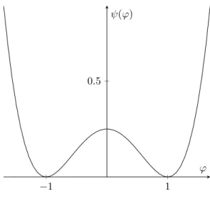
where ε and β are positive parameters related to the interfacial thickness and surface tension, respectively. The non-negative function ψ : R → R

is of double-well structure with two minima in or near the pure phases ϕ = ±1. Typical examples are the logarithmic potential ψ

which was originally proposed by Cahn and Hilliard [32], the double obstacle potential ψ

, and the smooth double-well potential ψ which is an approximation of both ψ

and ψ

. They are defined by

ψ

(r) =

(ln(1 + r)(1 + r) + ln(1 − r)(1 − r)) +

(1 − r

) ∀ r ∈ (−1, 1), ψ

(r) =

(

2

(1 − r

) for |r| ≤ 1,

+∞ else, ψ(r) =

(1 − r

)

,

with positive constants 0 < θ < θ

. The term

ψ(ϕ) favours the pure phases ϕ = ±1 while the gradient term penalises too rapid spatial changes of ϕ. In the absence of velocity and source terms, the mass balance law and the Ginzburg–Landau energy lead to the famous Cahn–Hilliard equation in which the flux is given by

J

= −m(ϕ)∇µ where µ = −βε∆ϕ + β ε ψ

(ϕ)

for a non-negative mobility function m(ϕ). The Cahn–Hilliard equation has been derived in the seminal work [32] by Cahn and Hilliard and has been studied by several authors, see, e. g., [19, 20, 31, 33, 61, 62]. Originally introduced to model phase separation in binary alloys, the Cahn–Hilliard equation has become one of the most popular phase field models with various applications like for example image inpainting (see [15, 36, 88]), two-phase flow (see [3, 21]), topology optimisation (see [17, 18]) and tumour growth.

A common feature that a tumour shares with any other living tissue is the requirement of

nutrient supply in order to grow. Consequently, we need to account for an additional species

1 Introduction 3 like oxygen or glucose in our model. Following the approach in [119], the conservation law and the energy contribution for the unknown species σ acting as a nutrient read as

∂

σ + div(σv) + div(J

) = −Γ

, N (ϕ, σ) = χ

2 |σ|

+ χ

σ(1 − ϕ),

where J

is a diffusive flux, Γ

is a term related to sources or sinks, and χ

, χ

are non- negative constants referred to as nutrient diffusion and chemotaxis parameter. By N we denote the nutrient free energy density which consists of one part which increases the energy in the presence of nutrients and another part referred to as chemotaxis energy and accounting for interactions between the nutrient and the tumour. As before, we may identify the flux as J

= −n(ϕ)(χ

∇σ − χ

∇ϕ) where n(·) is a non-negative mobility function, and the chemical potential µ has to be extended by adding a chemotaxis term −χ

σ which drives the tumour towards regions with higher nutrient concentration. We can now write our system as

∂

ϕ + div(ϕv) = div(m(ϕ)∇ −βε∆ϕ + βε

ψ

(ϕ) − χ

σ ) + Γ

,

∂

σ + div(σv) = div(n(ϕ) (χ

∇σ − χ

∇ϕ)) − Γ

.

Models of this form are referred to as Cahn–Hilliard type models and have been studied in the absence of velocity, that is, setting v = 0, in many contributions like for example [39, 74, 82, 85, 101, 103]. For mixtures consisting of more than two components it is more suitable to describe tumour growth dynamics by so-called multiphase Cahn–Hilliard type models, see, e. g., [13, 47, 67, 76, 86, 120, 137]. These models are more realistic if, for example, the tumour undergoes necrosis.

However, neglecting the velocity may be too restrictive since living biological tissues in general exhibit viscoelastic properties, see [78, 79, 125]. As pointed out in [64, 66], it is reasonable to consider Stokes flow as an approximation of certain types of viscoelastic behaviour since relaxation times of elastic materials are rather short (see [79]). Therefore, many authors used Stokes flow to describe the tumour as a viscous fluid, see [30,35, 65,68,71]. Classically, as pointed out earlier, velocities in tumour growth models are modelled with the help of Darcy’s law. In these models the velocity is assumed to be proportional to the pressure gradient caused by the birth of new cells and by the deformation of the tissue, see [26, 66, 96]. Brinkman’s law now interpolates between the viscous fluid and the Darcy-type models, see for example [51, 121, 134, 143], and can be derived from the momentum balance law when neglecting inertial effects. In the context of tumour growth this is a reasonable assumption since the Reynolds number is quite small.

Brinkman’s law was first proposed in [24] and has been derived rigorously by several authors using a homogenisation argument for the Stokes equation, see [10,124]. In this thesis, the general form of Brinkman’s law including adhesion forces is given by

−div(2η(ϕ)Dv + λ(ϕ)div(v)I − pI) + ν(ϕ)v = −βεdiv(∇ϕ ⊗ ∇ϕ), div(v) = Γ

, where Dv :=

(∇v+ (∇v)

) is the symmetrised velocity gradient, p is the pressure, and η(·), λ(·) and ν(·) are non-negative functions related to shear and bulk viscosity as well as permeability.

Moreover, the source term Γ

can be derived from single species laws and is usually closely related to Γ

. Brinkman’s law can be interpreted as an interpolation between Stokes flow and Darcy’s law since the former one is approximated on small length scales whereas the latter one on large length scales, see [53].

Summarising the above equations we obtain a coupled Cahn–Hilliard–Brinkman system for

tumour growth which serves as the basis for this thesis and is given by

div(v) = Γ

in Ω × (0, T ) =: Ω

,

−div(T(ϕ, v, p)) + ν (ϕ)v = −div(βε∇ϕ ⊗ ∇ϕ) in Ω

,

∂

ϕ + div(ϕv) = div(m(ϕ)∇µ) + Γ

in Ω

, µ = βε

ψ

(ϕ) − βε∆ϕ − χ

σ in Ω

,

∂

σ + div(σv) = div(n(ϕ)∇(χ

σ − χ

ϕ)) − Γ

in Ω

,

(1.1)

where Ω ⊂ R

, d = 2, 3, is a bounded domain, T > 0 is a fixed final time and T(ϕ, v, p) := 2η(ϕ)Dv + λ(ϕ)div(v)I − pI

is called the viscous stress tensor. In most parts of the thesis, we will supplement the system (1.1) with initial and boundary conditions of the form

∇ϕ · n = ∇µ · n = 0 on ∂Ω × (0, T ) =: Σ

,

∇σ · n = K(σ

− σ) on Σ

, T(ϕ, v, p)n = 0 on Σ

,

ϕ(0) = ϕ

, σ(0) = σ

in Ω,

(1.2)

where ϕ

, σ

and σ

are given functions, ∂Ω is the boundary of Ω and K ≥ 0 is a constant related to the boundary permeability.

We will refer to (1.1)-(1.2) as the full model. In many parts of this thesis, we will use a so-called quasi-static nutrient equation given by

0 = ∆σ − Γ

in Ω

. (1.3)

This seems to be more realistic from the modelling point of view since the timescale of nutrient diffusion is usually quite small compared to the tumour doubling timescale. For contributions in direction of the classical Cahn–Hilliard–Brinkman system, i. e., without source terms and nutrients, we refer to [21,42] for the local model and [49,50] for the non-local model. Moreover, we mention the recent work [77] where they studied a (non-)local Cahn–Hilliard–Darcy–Forchheimer–

Brinkman model for tumour growth.

In the following, we will outline the main novelties and difficulties of our model.

• A very important feature of our model is that the source term Γ

may depend on ϕ and σ. Although this condition is of high practical relevance due to the relation between Γ

and Γ

, many authors have worked with prescribed source terms Γ

not depending on variables of the diffuse interface model, see e.g. [81, 105]. This is related to the fact that boundary conditions of the form

v = 0 on ∂Ω or v · n = 0 on ∂Ω require a source term Γ

which fulfils the compatibility condition

Z

Ω

Γ

dx = Z

Ω

div(v) dx = Z

∂Ω

v · n dH

= 0.

Also in the case of inhomogeneous boundary conditions in the form given above, a

compatibility condition has to be satisfied. In the case of a solution dependent source

term, it is in general not possible to fulfil such a condition. In the literature, there are only

a few contributions in this direction, see, e. g. [47, 83], where they consider a quasi-static

nutrient equation. To the author’s best knowledge, there is no contribution concerning

existence of weak solutions for Cahn–Hilliard type models for tumour growth with solution

dependent source terms, velocity effects and with a nutrient equation of the form (1.1)

.

1 Introduction 5

• The term T(ϕ, v, p)n characterises effects due to friction on the boundary. The boundary condition (1.2)

is one of the main features of our model and can be referred to as a

“no-friction” condition. It allows us to consider solution dependent source terms and is quite useful in applications, see [95, App. III, 4.4], and very popular for finite element discretisations of the Navier–Stokes equation since it appears naturally in the variational formulation of (1.1)

. In numerical simulations, it can be used to implement boundary conditions in an unbounded domain, for example a channel of infinite length. In this context, we also want to refer to the so-called classical “do-nothing” boundary condition

∂v

∂n − pn = 0,

see, e. g., [102]. To the author’s best knowledge, there are no contributions in the literature for Cahn–Hilliard-type models for tumour growth with the no-friction boundary condition

• The presence of source terms causes several new difficulties in the analysis. In particular, the most important properties of the classical Cahn–Hilliard equation are not fulfilled by our model, like the decrease of energy and the mass conservation property for ϕ, and classical arguments for the analysis do no longer work. Crucial in the analysis is the estimate for the chemical potential which requires a bound on the mean of µ to apply Poincaré’s inequality. However, the mean of µ is related to the growth of the potential ψ(·) and therefore classical singular potentials cannot be included in the analysis in general. In many contributions, the potential is required to grow at most quadratically, see, e. g., [81–83]. We will apply a new estimate that allows us to consider potentials with higher order growth in some situations and, in particular, can be applied to the classical double-well potential. Moreover, we remark that the velocity is not divergence free and thus classical arguments for Stokes-like equations do not apply since the pressure cannot be eliminated in the weak formulation.

Structure of the thesis We will now outline the structure of this thesis.

A fundamental biological and mathematical background is provided in Chapter 2. In the first part we will introduce the biological notions and aspects related to tumour growth. In the second part we provide auxiliary results that will be applied in this thesis. Most of them are concerned with Galerkin schemes and the analysis of Brinkman or Stokes subsystems. We will give a detailed proof for weak and strong solutions of the Brinkman subsystem with solution dependent viscosities and permeability supplemented with Neumann-type boundary conditions for the stress tensor. The corresponding results seem not to be available in the literature in this form and may therefore be of independent interest.

In Chapter 3 we first derive the diffuse interface model using thermodynamic principles, consti- tutive assumptions, balance laws for mass and momentum, and the Lagrange multiplier method.

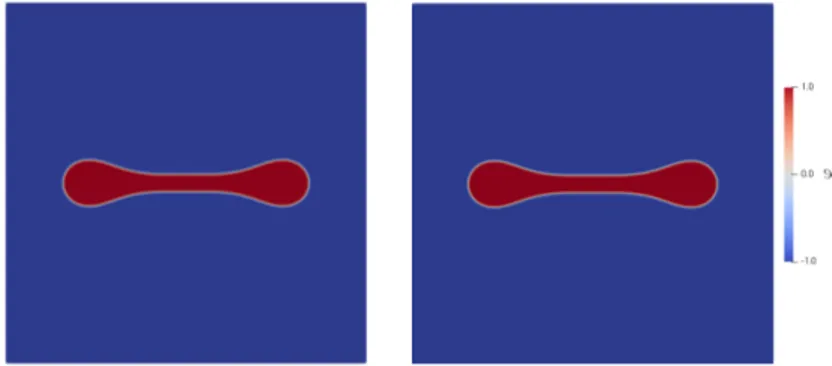
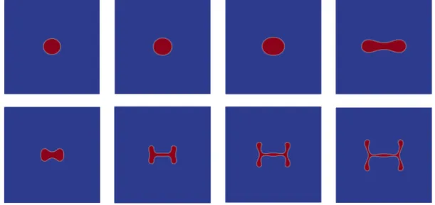
We then discuss further aspects of modelling and we use the method of formally matched asymptotics in order to relate our model with free boundary problems for tumour growth that appeared earlier in the literature. Lastly, we will present numerical simulations which give insights into the qualitative behaviour of the model. The simulations have been made by Robert Nürnberg from Imperial College London (see [56]).

Existence of weak solutions for the full model in a very general setting will be established in Chapter 4. The proof is based on a Galerkin approximation, on energy estimates and compactness arguments. The chapter is based on the work [54].

Partial results of the work [55] will be presented in Chapter 5. More precisely, we will prove

well-posedness and existence of strong solutions for the model with quasi-static nutrient equation.

This will serve as the basis for the optimal control problem which we study in Chapter 9. We point out that the analysis includes the classical double-well potential which is the standard smooth potential used in the literature.

In Chapter 6 we analyse several singular limits of the model with quasi-static nutrients. We remark that the results for three dimensions are part of the work [55]. In the limit of large boundary permeability, i. e., sending K → ∞ in (1.2)

, we recover weak solutions with a Dirichlet boundary condition for σ. More interestingly, we investigate the zero viscosity limit in the Cahn–Hilliard–Brinkman system (CHB) which allows us to relate our model to former Cahn–Hilliard–Darcy models (CHD) for tumour growth in the literature, see, e. g., [83]. In three space dimension we can show that weak solutions of the CHB model converge to a weak solution of the CHD model. In two space dimensions, we show that strong solutions of the CHB model converge to strong solutions of the CHD system. In particular, we establish uniqueness of weak solutions for the CHD tumour model and we prove a qualitative estimate between strong solutions of the CHB and CHD models in a similar fashion as in [21]. We remark that the CHD model without source terms and nutrient is referred to as Cahn–Hilliard–Hele–Shaw system and has been investigated in, e. g., [48, 63, 112].

A variant of the CHB model with one-sided degenerate mobilities and singular potentials will be analysed in Chapter 7. The mobility degenerates in ϕ = −1 and we allow for a singularity of ψ(·) in ϕ = −1. Typical examples are so-called single-well potentials of Lennard–Jones type, see, e. g., [5, 6]. In contrast to the rest of this thesis, we consider a no-slip boundary condition for the velocity and we set Γ

= 0, i. e.,

div(v) = 0 a. e. in Ω

, v = 0 a. e. on Σ

.

We establish the existence of weak solutions for the full model based on arguments in [62].

However, we cannot apply the ideas directly since solutions for the non-degenerate mobility are not regular enough in order to justify a testing procedure in the style of [62]. Our idea is to add a regularisation term δ∂

v, δ > 0, in the Brinkman equation in order to obtain more regular solutions for the system with non-degenerate mobility. We then regularise potential and mobility with the same parameter δ and establish estimates independent of δ > 0 which allows us to obtain solutions for the degenerate mobility by sending δ → 0. Due to the no-slip boundary condition, the result remains valid for the Stokes equation since estimates can be obtained independent of the permeability ν. Our result seems to be the first for local Cahn–Hilliard type models for tumour growth with source terms and degenerate mobility. For the non-local version, we refer to [75] where they consider a two-sided degenerate mobility.

Under certain conditions on the source terms we can establish existence of solutions for the model with quasi-static nutrients and singular potentials, see Chapter 8. The results are part of the work [59] and include the logarithmic and double obstacle potential which are the most relevant examples. For our analysis it suffices to prescribe conditions on Γ

and Γ

in the pure phases ϕ = ±1. In order to control the source terms we come up with a new estimate which allows us to bound the convex parts of the regularised potentials on the boundary independent of the regularisation parameter. We use the ideas presented in the work [88] to control the mean of ϕ since classical arguments as in [19] fail which is due to the fact that mass is not conserved. By sending the viscosities to zero we establish the corresponding results for the CHD model. Finally, we prove existence of solutions for the stationary model without velocity.

In the context of Cahn–Hilliard type models with singular potentials and source terms we

mention the works [76, 85], where the first one is in the absence of velocity and with Dirichlet

boundary conditions and the second one considers a multi-phase model with a different boundary

condition for µ. We point out that our methods can be used in a similar fashion for the so-called

Cahn–Hilliard–Oono equation, see [93], and for models with applications to image inpainting,

1 Introduction 7 see [15, 88].

Finally, in Chapter 9 we study an optimal control problem where the medication by cytotoxic drugs acts as the control. The results are part of the contributions [57, 58]. We modify the nutrient equation by adding a term that models the supply of nutrients from an existing vasculature and we impose a Neumann boundary condition, i. e.,

0 = ∆σ + B(σ

− σ) − Γ

in Ω

, ∇σ · n = 0 on Σ

,

where B is a positive constant and σ

is a given nutrient supply from the vasculature. We

establish the fundamental requirements of calculus of variations, the existence of a global optimal

control and first order necessary optimality conditions. Similar results have been obtained for

classical Cahn–Hilliard models in [16, 38, 41, 91, 104, 141, 142] and Cahn–Hilliard type models for

tumour growth in, e. g., [40, 84, 106, 128–130]. In the last part of the chapter we establish second

order sufficient conditions for local and global optimality. Finally, we investigate local and global

uniqueness of optimal controls. To the author’s best knowledge, this is the first contribution

regarding second order optimality conditions for Cahn–Hilliard type models for tumour growth.

2

Biological and mathematical background

2.1 Fundamental biological aspects of tumour growth

In this section we present basic notions of biology which play a key role to understand mecha- nisms and processes related to tumour growth. Since the biology of humans and the inherent mechanisms in the human body are extensive and complicated, giving a complete description of cancer biology is far beyond the scope of this work. However, we aim to describe the key mechanisms and structures needed to understand the models we consider in this work. Once we have sketched the typical tissue structure, we will describe the different stages of tumour growth, from early stages where the tumour mainly grows by consuming nutrients from the surrounding environment, to later stages where the tumour has built its own vascular system. This part is inspired by and collected from the very well written and detailed biological textbooks [9, 109]

and the work [45].

2.1.1 The tissue structure

Basically, we can subdivide the tissue into four groups (see [109, Chap. 1.2]).

(i) The supporting tissue called mesenchyme consisting of connective tissue like fibroblasts (which make collagen and elastin fibres as well as associated proteins), blood vessels, lymphatics, bone, cartilage and muscles; the stroma contains, e. g., the fibroblasts, blood vessels, lymphatics or collagen fibres, and is a part of the mesenchyme. The extracellular matrix (ECM) builds the main part of the stroma and consists of fibres like collagen or elastin surrounded by water and proteins.

(ii) The tissue-specific cells called epithelium – these are the specific cells of different organs like, e. g., skin, intestine or liver.

(iii) The haematolymphoid system consisting of ‘defence’ cells like lymphocytes, macrophages or lymphoid cells.

(iv) The nervous system which is divided into the central and peripheral nervous system,

9

the first one consisting of the brain and spinal cord whereas the latter is comprised of nerves leading from the central system.

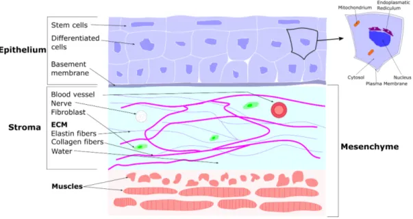
Structure and function of individual tissues are maintained by tissue-specific cells that are arranged in a standard pattern (see Figure 2.1 and [109, Figure 1.1]). Tissue-specific cells are grouped in a layer of epithelium, separated by a semipermeable basement membrane from the mesenchyme. The connective tissue consists mainly of the stroma which may be supported by a layer of bones or muscles, and is supplied with, for example, nutrients and nervous control by blood and lymphatic vessels or nerves, depending on the tissue-specific needs.

Figure 2.1: Typical tissue structure.

The epithelium mainly consists of two cell-types.

(i) Differentiated cells usually only differentiate into a specific type of cell which is due to a so-called cell memory phenomenon. The cells remember changes in gene expression and maintain their choice through subsequent cell generations, see [9, Chap. 7, p. 454].

(ii) Stem cells are specialized cells and provide an indefinite supply of new differentiated cells if those are, for example, lost or discarded, see [9, Chap. 23, p. 1417].

The structure of both differentiated and stem cells can basically be divided into three parts (see [45, Sec. 2.1.3]). The inner part consists of the nucleus that contains the cell’s DNA.

It is surrounded by the so-called cytoplasm consisting mainly of the cell liquid cytosol and containing organelles carrying out the functions of the cell, like, for example, mitochondria and endoplasmic reticulum.

Each cell is enclosed by a semi-impermeable plasma membrane separating the cytoplasm from

the surrounding extracellular tissue and containing proteins that transfer information across the

membrane, possibly triggering a changing behaviour of the cell. Moreover, the plasma membrane

keeps the nutrient gathered in the cell and excretes waste products into the environment. For

more information, see [9, Chap. 1].

2.1 Fundamental biological aspects of tumour growth 11

2.1.2 Tumour growth as a multistage process

We first need to explain some crucial terms that are involved during the whole process.

Growth and proliferation (see [109, Chap. 1.3]): Although the term growth is often used for both of these processes, it is important to distinguish these two processes in the context of tumour growth.

We use the term growth to describe an increase of, for example, cell, tissue or tumour size. It is worth mentioning that there is a very precise mechanism allowing individual organs to reach a certain size which is usually never exceeded.

The term proliferation here means an increase of cell number realised by division. In the case that a part of the tissue is injured, damaged cells are replaced by division (proliferation) of the surviving cells. This process is mostly completed by special reserve or stem cells which can divide in order to substitute organ-specific cells. Proliferation is a multi-stage process and involves in particular the final stage called mitosis where two copies of the DNA are separated and two nuclei with this new DNA emerge.

Apoptosis (see [109, Chap. 12.2]) is the process of programmed cell death. Understanding this mechanism is of high importance for cancer researchers to develop new effective strategies and medicines since the effectiveness of, e. g., drug-based cytotoxic cancer therapy relies on the ability to kill cancer cells by inducing apoptosis.

In normal tissue – at least in an adult body – proliferation and apoptosis are rather balanced.

As explained above, once a cell is injured or its DNA is damaged, the process of controlled cell death (apoptosis) starts and the damaged cell is replaced by a new one via proliferation.

The early stages - avascular tumour growth (see [45, Chap. 2.2.1 - 2.2.3])

In order to describe the early stages of tumour growth it is important to understand the effects that trigger the initial growth phase. The initial formation of tumour tissue is a multistage process referred to as carcinogenesis.

It starts with a genetic mutation of normal cells which triggers the formation of one or a small colony of tumour cells. If these mutations can overcome their natural repair mechanisms, they can further mutate which enables them to ignore neighbouring signals that would inhibit their growth.

In such a case the colony reaches the next stage of carcinogenesis in which low apoptosis favours the formation of a highly proliferative tumour colony. This ensemble of cells is referred to as in situ cancer, that means, it is situated in the epithelium and is usually rather small. It is more likely that the colony develops by mutations of stem cells rather than differentiated cells, since the latter ones are restricted in proliferation and cannot divide unlimited. In fact, after a limited number of divisions, differentiated cells either rest in an quiescent state or die by apoptosis.

In conclusion, the evolution of an initial tumour colony is mostly triggered by an imbalance of low apoptosis and high or fast cell proliferation.

At that time the young tumour colony does not have its own vascular system and must therefore consume growth factors and vital nutrients like oxygen or glucose from the surrounding stroma.

Nourishment diffuses from the vascularized stroma, enters the epithelium where the tumour

is located, and is uptaken by the cancerous cells to proliferate rapidly. As the extent of the

tumour ensemble increases, cells in the middle are affected by hypoxia which means that they

suffer from an undersupply of vital oxygen and, as a consequence, their rate of proliferation and

the growth rate of the tumour declines, see [27]. If the concentration of oxygen or glucose in

the tumour centre becomes smaller than a critical value, these cells undergo necrosis, that is,

Figure 2.2: Structure of the tumour after necrosis, see also [140, Scheme 1].

uncontrolled and unplanned cell death due to a lack of nutrients. Once the process of necrosis has started, the tumour typically consists of three layers: a necrotic core, a region of quiescent cells which do not proliferate, and an outer viable rim of proliferating tumour cells, see Figure 2.2.

Apart from vascularization which will be described later on, there are other mechanisms that allow the tumour to overcome nutrient limitation. By interacting with its environment, the tumour can mechanically displace or compress its surroundings like the basement membrane.

For instance, the tumour can release enzymes to degrade and remodel the ECM which possibly creates new fuel for growth. Degradation of the ECM leads to additional space and reduced pressure in the tumour’s micro-environment. As a result the tumour invades and may undergo morphological instabilities like fingering or folding along the directions of low mechanical pressure, see, for example, [44, 46].

A similar effect is observed during chemotaxis, describing the movement (of the tumour) towards regions with higher concentrations of a soluble substrate (like oxygen) along the concentration gradient. In this context we also mention a process called haptotaxis, describing the movement towards directions with higher concentrations of a substrate-bound (chemo-)attractant.

Moreover, some tumours can mutate in order to build active glucose transporters (e. g., SGLTs) on their cell membrane to be independent of nutrient diffusion (so-called passive transport).

These transporters trigger the movement of, for example, glucose towards the tumour colony even against the gradient of nutrient concentration. Such a process is referred to as active transport.

For more information regarding chemotaxis and active transport, see, for example, [87] and the references therein.

The vascularization stage (see [9, Chap. 23], [45, Chap. 2.2.4])

During the process of vascular growth new capillary vessels are developed by sprouting or division from the pre-existing host vasculature. This process is referred to as angiogenesis and it is responsible for permanent remodelling and extension of the capillary network. It occurs during the whole life-time of a human being and mostly occurs if a part of the tissue suffers from a lack of blood supply and sends out complex signals, in particular so-called vascular endothelial growth factors (VEGFs), in order to trigger the growth of new vessels.

Every vessel consists of a lumen surrounded by a shin sheet of endothelial cells which play a

2.2 Notation 13 crucial role during the process of angiogenesis, and a basal lamina separating the vessel from the surrounding outer layers.

Once the size of a tumour gets big enough, interior cells suffer from hypoxia. Those hypoxic cells produce hypoxia-inducible factors (HIFs) stimulating the transcription and secretion of so-called tumour angiogenic growth factors (TAFs) like VEGFs. As the VEGF proteins diffuse from the hypoxic region, a VEGF gradient emerges. Once the endothelial cells of the vessel detect this gradient they are stimulated to proliferate and they secrete proteins in order to find a way through the basal lamina. A new capillary forms, directed towards the VEGF source via chemotaxis or haptotaxis, and this new capillary links with another existing vessel or capillary, resulting in a new vasculature providing direct oxygen or nutrient supply to the cancer tissue and allowing for rapid growth of the tumour. For a more detailed description of this process, we refer, for example, to [9, Chap. 23].

In well-oxygenated tissue there are enzymes that switch of the production of, for example, HIFs once the new capillary has formed. However, this may not be the case in tumour tissue where new vessels can evolve even if the cells are well-supplied with oxygen or nutrients. Those new vessels may be less efficient, their neovasculature may be leaky, less stiff or collapsing when faced with tissue stress, and the basal lamina may have defects. As a consequence, drug therapy may be inefficient since drugs may not reach the tumour tissue.

The last stage in the process of tumour growth is referred to as metastasis and commonly causes death. It involves many complex phenomena, like, for example, genetic instabilities, increasing HIF production and loss of cell-cell adhesion. The tumours invade their surroundings and may develop secondary cancers. In many cases lymphatic vessels build the basis to enable the tumour escaping from its primary organ. Some of the cancer cells are transported to and arrested by lymph nodes. They may be destroyed or they build new tumours. The process of metastasis can also be a result of tumour cells entering blood vessels and moving to other organs.

It is worth mentioning that, although being the most harmful stage, metastasis is still poorly understood. We refer to [45] and references therein for more information regarding this process.

2.2 Notation

We first fix some notation. Throughout this thesis we denote by Ω ⊂ R

, d = 2, 3, a bounded domain with boundary ∂Ω, and by T > 0 a fixed final time. We denote Ω

:= Ω × (0, T ), Σ

:= ∂Ω × (0, T ), and for t ∈ (0, T ) we write Ω

:= Ω × (0, t). For a (real) Banach space X we denote by k·k

its norm, by X

the dual space, and by h · , · i

the duality pairing between X

and X . For an inner product space X the inner product is denoted by ( · , · )

. We define the scalar product of two matrices by

A : B :=

d

X

j,k=1

a

b

for A, B ∈ R

, and the divergence of a matrix by

div(A) :=

d

X

k=1

∂

a

(x)

!

j=1

∀ A ∈ R

.

By n we will denote the outer unit normal on ∂Ω. For the standard Lebesgue and Sobolev

spaces with 1 ≤ p ≤ ∞, k > 0, we use the notation L

:= L

(Ω) and W

:= W

(Ω) with

norms k·k

and k·k

, respectively. In the case p = 2 we use H

:= W

and the norm

k·k

. For β ∈ (0, 1) and r ∈ (1, ∞) we will denote the Lebesgue and Sobolev spaces on the

boundary by L

(∂Ω) and W

(∂Ω) with corresponding norms k·k

and k·k

(see, e. g., [133, Chap. I.3] for more details). In the case r = 2 we use H

(∂Ω) := W

(∂Ω). We denote the space W

as the completion of C

(Ω) with respect to the W

-norm and we set H

:= W

. By L

, W

, H

, L

(∂Ω), H

(∂Ω), W

(∂Ω), W

and H

we will denote the corresponding spaces of vector valued and matrix valued functions. For Bochner spaces we use the notation L

(X ) := L

(0, T ; X ) for a Banach space X with p ∈ [1, ∞]. If X = L

we will sometimes identify L

(0, T ; L

) with L

(Ω

). We define

k·k

:= k·k

+ k·k

for two or more Bochner spaces A and B. For the dual space X

of a Banach space X we introduce the (generalised) mean value by

v

:= 1

|Ω|

Z

Ω

v dx for v ∈ L

, v

:= 1

|Ω| hv ,1i

for v ∈ X

. Moreover, we introduce the function spaces

L

:= {w ∈ L

: w

= 0}, (H

)

:=

f ∈ (H

)

: f

= 0 , H

:=

w ∈ H

: ∇w · n = 0 on ∂Ω .

For problems related to the Stokes equation we define the space of smooth and divergence-free vector fields with compact support in Ω by

V :=

v ∈ C

(Ω; R

) : div(v) = 0 , and we define

H := V

2

, V := V

1

.

Then, it is well-known (see, e. g., [22, Lem. IV.3.4, Thm. IV.3.5]) that V =

v ∈ H

: div(v) = 0 and H =

v ∈ L

: div(v) = 0, v · n = 0 on ∂Ω . Finally, for 1 < q < ∞ we define L

(Ω) := {f ∈ L

: div(f ) ∈ L

}

equipped with the norm

kf k

div(Ω)

:= (kf k

+ kdiv(f )k

)

, where div is the weak divergence.

2.3 Auxiliary results

We divide this section into several parts which are related to specific topics in this thesis. First, we recall some general results.

2.3.1 General auxiliary results

We start by stating the following generalised version of Hölder’s and Young’s inequalities:

Lemma 2.1 Let Ω ⊂ R

, d ≥ 1, be a bounded domain. Let v ∈ L

, 1 ≤ p ≤ ∞, and w ∈ L

, 1 ≤ q ≤ ∞. Then the product vw belongs to L

where

1 r = 1

p + 1 q , and

kvwk

≤ kvk

kwk

. (2.1)

2.3 Auxiliary results 15

Lemma 2.2 Let a, b ∈ R and p, q ∈ (1, ∞). Then, for every δ > 0 it holds

|ab| ≤ δ|a|

+ (δp)

q |b|

with 1 p + 1

q = 1. (2.2)

Proof. We follow the arguments in [11, proof of Lem. 1.14]. Without loss of generality, we assume a, b > 0. Concavity of the logarithm yields

ln(ab) = ln(a) + ln(b) = 1

p ln(a

) + 1

q ln(b

) ≤ ln 1

p a

+ 1 q b

= ⇒ ab ≤ 1 p a

+ 1

q b

. Therefore, for δ > 0 we have

ab = (pδ)

a 1

(pδ)

b ≤ δa

+ 1 q

(pδ)

b

= δa

+ (δp)

q b

, and the proof is complete.

We recall Poincaré’s inequality with mean value for H

.

Lemma 2.3 (see [80, Thm. II.5.4]) Let Ω ⊂ R

, d ≥ 2, be a bounded domain with Lipschitz- boundary. Then, for all f ∈ W

, 1 ≤ q < ∞ there exists a constant C

depending only on Ω, q and d such that

kf k

≤ C

(k∇f k

+ |f

|) ∀ f ∈ W

, (2.3a) or equivalently

kf − f

k

≤ C

k∇f k

∀ f ∈ W

. (2.3b) Furthermore, we will use the following generalised Gagliardo–Nirenberg inequality:

Lemma 2.4 Let Ω ⊂ R

, d ≥ 2, be a bounded domain with Lipschitz boundary and for m ∈ N , 1 ≤ q, r ≤ ∞, let f ∈ W

∩ L

. Moreover, consider any integer j ∈ [0, m) and any θ ∈

m

, 1 such that there exists p ∈ [1, ∞] satisfying

j − d p =

m − d

r

θ + (1 − θ)

− d q

.

If r ∈ (1, ∞) and m − j −

is a non-negative integer, we assume in addition that θ < 1. Then there exists a positive constant C depending only on Ω, d, m, j, p, q, r and θ such that

kD

f k

≤ Ckf k

kf k

. (2.4) Proof. See, e. g., [4, Thm. 5.8], [118, Thm. 1] and references therein.

In the following we introduce the notions of linear and compact operators as well as (bi-)dual spaces.

Definition 2.5 (see [11, Sec. 3.2, Def. 3.5 and Sec. 6.2]) Let X, Y be normed K -spaces where K ∈ { C , R }. Then, we define the set of linear operators by

L(X, Y ) := {S : X → Y | S is linear and continuous} , and the set of compact operators by

K(X; Y ) := n

S ∈ L(X, Y ) | S(B

(0)) is compact in Y o .

The dual space of X is defined by X

:= L(X; K ) and the bi-dual space by X

:= (X

)

.

Lemma 2.6 (see [11, Sec. 6.2.1]) Let X be a normed space. Then the mapping J

∈ L(X ; X

) defined by

hJ

(x), x

i

:= hx

, xi

∀ x

∈ X

is an isometry. In particular, it holds that

kxk

= sup

x^∗∈X^∗\{0}

hx

, xi

kx

k

. (2.5)

Lemma 2.7 (see [11, Sec. 10.1]) Let X, Y be normed spaces. Then the mapping

: L(X, Y ) → L(Y

, X

) which assigns to S ∈ L(X, Y ) an operator S

∈ L(Y

, X

) defined via

hS

y

, xi

:= hy

, Sxi

∀ x ∈ X, y

∈ Y

(2.6) is an isometric embedding. The operator S

∈ L(Y

, X

) is called dual or adjoint operator of S ∈ L(X, Y ).

Theorem 2.8 (Schauder, see [11, Thm. 10.6]) Let X, Y be Banach spaces and S ∈ L(X; Y ).

Then it holds

S ∈ K(X, Y ) ⇐⇒ S

∈ K(Y

, X

).

Lemma 2.9 Let X, Y be separable Banach spaces such that X is densely and continuously embedded into Y , i. e., there exists a continuous embedding i : X → Y such that i(X )

= Y . Then, Y

is continuously embedded into X

. Moreover, if X is reflexive, the embedding is dense.

Proof. First, we note that i

∈ L(Y

, X

). Let f ∈ Y

such that i

(f ) = 0. Then, it follows by definition that hf , i(x)i

= 0 for all x ∈ X and since i(X )

= Y , this implies f = 0.

Consequently, i

is injective which yields the first assertion.

Now, let X be reflexive and let h ∈ X

such that h(i

(f )) = 0 for all f ∈ Y

. Then, there exists x ∈ X such that J

(x) = h and

0 = hh , i

(f )i

= hJ

(x) , i

(f )i

= hi

(f ), xi

= hf , i(x)i

∀ f ∈ Y

.

Since i is injective and by (2.5), this implies x = 0, hence h = J

(x) = 0. Therefore, we infer that

h(i

(f )) = 0 ∀ f ∈ Y

= ⇒ h(x

) = 0 ∀ x

∈ X

. By the Hahn–Banach theorem we obtain i

(Y

)

∗

= X

which completes the proof.

2.3.2 Results related to Galerkin schemes

Galerkin schemes are a common approach to prove existence of solutions for PDE systems. The procedure can roughly be described as follows:

(i) construct a Schauder basis by means of eigenfunctions of a certain differential operator.

(ii) solve the PDE system on finite dimensional subspaces given by the span of eigenfunctions.

For time-dependent problems, this mostly can be done by solving a system of (non-linear) ODEs.

(iii) prove that solutions are independent of the dimension of the finite dimensional subspaces.

(iv) use compactness arguments to recover the solution of the original problem when passing to the limit in the approximating system.

In the following we will present auxiliary results related to the individual steps of the Galerkin

scheme.

2.3 Auxiliary results 17

Construction of a Schauder basis – the Neumann–Laplace operator

In this part we assume that Ω ⊂ R

, d ≥ 2, is bounded domain. We begin with the following definition:

Definition 2.10 The Neumann–Laplace operator −∆

: H

→ (H

)

is defined through h−∆

u , vi

:=

Z

Ω

∇u · ∇v dx ∀ u, v ∈ H

.

Remark 2.11 For arbitrary u ∈ H

, the element −∆

u belong to (H

)

since h−∆

u , 1i

=

Z

Ω

∇u · ∇1 dx = 0.

Lemma 2.12 The following statements hold true:

(i) for every f ∈ (H

)

there exists a unique u ∈ H

∩ L

such that −∆

u = f , (ii) for every g ∈ L

the mapping f : v 7→ (g, v)

defines an element f ∈ (H

)

.

Proof. We define the space V := H

∩ L

. Then, applying Poincaré’s inequality and the Lax–Milgram theorem, there exists a unique u ∈ V solving

Z

Ω

∇u · ∇v dx = hf, vi

∀ v ∈ V.

Since f ∈ (H

)

, this identity holds also for all v ∈ H

which implies (i).

Assertion (ii) follows due to Hölder’s inequality and the proof is complete.

In particular, the inverse operator (−∆

)

: (H

)

→ H

∩ L

is well-defined.

Lemma 2.13 Let w ∈ H

. Then, it holds

(−∆

)

(−∆

w) = w − w

. Proof. Setting f = −∆

w ∈ (H

)

, we obtain

hf , vi

= Z

Ω

∇w · ∇v dx = Z

Ω

∇(w − w

) · ∇v dx ∀ v ∈ H

.

Since w − w

∈ H

∩ L

, this implies (−∆

)

(−∆

w) = (−∆

)

f = w − w

which completes the proof.

Corollary 2.14 The following statements holds true:

(i) the embeddings H

⊂ H

⊂ L

' (L

)

⊂ (H

)

⊂ (H

)

are dense and continuous, (ii) the embeddings H

⊂⊂ H

⊂⊂ L

and (L

)

⊂⊂ (H

)

⊂⊂ (H

)

are compact.

Proof. (i): from standard Sobolev embedding theorems (see Lemma 2.32), it follows that H

⊂ H

⊂ L

with continuous embeddings. Moreover, it is well known that the embedding H

⊂ L

is dense. From [82, Lemma 3.1], we obtain that the embedding H

⊂ H

is dense.

Then, since H

, H

, L

are separable, reflexive Banach spaces, applying Lemma 2.9 yields that

the embeddings (L

)

⊂ (H

)

⊂ (H

)

are dense and continuous. Finally, the embedding

L

⊂ (L

)

is dense and continuous since L

is a separable Hilbert space.