Variational analysis of low-lying states in supersymmetric Yang-Mills theory

JHEP04(2019)150

Published for SISSA by Springer Received: January 21, 2019 Revised: March 15, 2019 Accepted: April 16, 2019 Published: April 24, 2019

Variational analysis of low-lying states in supersymmetric Yang-Mills theory

Sajid Ali,

^a,b

Georg Bergner,

^c,a

Henning Gerber,

^a

Simon Kuberski,

^a

Istvan Montvay,

^d

Gernot M¨ unster,

^a

Stefano Piemonte

^e

and Philipp Scior

^f

aInstitute for Theoretical Physics, University of M¨unster, Wilhelm-Klemm-Str. 9, D-48149 M¨unster, Germany

bDepartment of Physics, Government College University Lahore, Lahore 54000, Pakistan

cInstitute for Theoretical Physics, University of Jena, Max-Wien-Platz 1, D-07743 Jena, Germany

dDeutsches Elektronen-Synchrotron DESY, Notkestr. 85, D-22607 Hamburg, Germany

eInstitute for Theoretical Physics, University of Regensburg, Universit¨atsstr. 31, D-93040 Regensburg, Germany

fFaculty of Physics, University of Bielefeld, Universit¨atsstr. 25, D-33615 Bielefeld, Germany

E-mail: sajid.ali@uni-muenster.de, georg.bergner@uni-jena.de, h.gerber@uni-muenster.de, simon.kuberski@uni-muenster.de, montvay@mail.desy.de, munsteg@uni-muenster.de,

stefano.piemonte@ur.de, scior@uni-muenster.de

Abstract: We have calculated the masses of bound states numerically in N = 1 su- persymmetric Yang-Mills theory with gauge group SU(2). Using the suitably optimised variational method with an operator basis consisting of smeared Wilson loops and mesonic operators, we are able to obtain the masses of the ground states and first excited states in the scalar, pseudoscalar and spin- ½ sectors. Extrapolated to the continuum limit, the corresponding particles appear to be approximately mass degenerate and to fit into the predicted chiral supermultiplets. The extended operator basis including both glueball-like and mesonic operators leads to improved results compared to earlier studies, and moreover allows us to investigate the mixing content of the physical states, which we compare to predictions in the literature.

Keywords: Lattice Quantum Field Theory, Supersymmetric Gauge Theory

ArXiv ePrint: 1901.02416

JHEP04(2019)150

Contents

1 Introduction 1

2 Supersymmetric Yang-Mills theory on the lattice 3

3 Techniques for the determination of light states 4 3.1 Computation of the masses using the variational method 4

3.2 Interpolating operators 5

3.3 Stochastic estimator technique (SET) 6

3.4 Smearing techniques 7

4 Optimising the methods 8

4.1 Jacobi smearing 8

4.2 Presmearing of the gauge fields 8

4.3 Variational operator basis 10

4.4 Number of stochastic estimators 11

5 Extended variational basis 11

6 Supermultiplets 13

7 Mixing between glueballs and mesons 17

8 Conclusions 18

1 Introduction

The N = 1 supersymmetric Yang-Mills (SYM) theory is the minimal supersymmetric ex-

tension of the pure gauge sector of QCD, describing the strong interactions of gluons and

their fermionic superpartners, the gluinos. Unbroken supersymmetry requires the physical

bound states of N = 1 SYM to form supermultiplets of degenerate masses. Based on super-

symmetric effective actions, the lowest-lying supermultiplet has originally been proposed in

ref. [1] to be a chiral supermultiplet formed out of a scalar and a pseudoscalar meson and a

spin-½ bound state of gluons and gluinos, called gluino-glue. The original analysis has been

extended in refs. [2, 3] to include also glueball operators which can mix with the meson

operators carrying the same quantum numbers. The scalar and pseudoscalar bound states

are therefore created by linear combinations of meson-like and glueball-like operators. The

mass hierarchy and the amount of mixing are difficult to predict theoretically from the

effective Lagrangian and are in general unconstrained by supersymmetry.

JHEP04(2019)150

Numerical simulations of N = 1 SYM on a space-time lattice are required to verify and extend the analytical predictions about the low energy effective theory. The study of the lightest bound states of N = 1 SYM with SU(2) gauge symmetry has been the main subject of several publications by our collaboration [4–8]. The results reveal the expected degeneracy of the members of the chiral multiplet in the continuum limit. In particular, the scalar glueball and the scalar meson masses, extrapolated to the continuum limit, have compatible values, which hints at mixing of the states in this channel.

In the present work we have optimised our techniques to extract the masses with respect to our previous work. This allows for the first time to investigate the mixing properties of the two lowest supermultiplets from the lattice gauge ensembles we have generated. In this article we explain these methods and their optimisations. We show, in particular, that the construction of an enlarged correlation matrix including both, the meson and glueball oper- ators, is crucial to extract the physical states in the scalar channel. Using these techniques systematic errors stemming from excited state contributions can be controlled much better.

We reanalyse the gauge configurations of previous investigations yielding more reliable and more precise results for the lightest masses. In addition, we are able to extract the masses of excited states in the scalar, pseudoscalar, and fermionic channel. In this way we provide first results concerning the possible formation of a supermultiplet of excited states on the lattice.

The formation of supermultiplets at the level of the excited states is strong evidence for the fact that the unavoidable breaking of supersymmetry on the lattice can be kept under control. The states with higher masses are affected stronger by lattice artefacts, and hence the predicted degeneracy of these states is more sensitive to the breaking of supersymmetry on the lattice. The present work represents the first step towards an investigation of the spectrum of excited states of N = 1 SYM. An alternative determination of supersymmetry violations beyond the ground state level would be the weighted sum of all energy differences in terms of the derivative of the Witten index, see [9].

In addition to our results on excited states, we confirm our earlier results concerning the mixing of glueball and meson operators in the ground state, and we are able to determine the glueball and the meson contents. Eventually this might lead to a better understanding of the conjectures concerning the low energy multiplets of the theory.

In this work we have optimised our methods for SYM with gauge group SU(2). The techniques are, however, also suitable for other theories. Currently we are applying the same methods successfully to SYM with gauge group SU(3), for which the results will be published soon. Our techniques are also applicable to lattice QCD, where similar investi- gations are being done.

It should be noted that our studies, and corresponding investigations in QCD as well, are quite challenging due to the noisy signals from glueball operators and the disconnected meson contributions.

This paper is organised as follows: N = 1 SYM in the continuum and on the lattice is

introduced in the next section. The current paper is particularly focused on the technical

aspects, which are explained in sections 3, 4, and 5. The physical results, the improved

signal for the ground states, the mixing, and the excited states, are finally presented in

sections 6 and 7.

JHEP04(2019)150

2 Supersymmetric Yang-Mills theory on the lattice

The Lagrangian L of the N = 1 SYM in Euclidean space-time, L = 1

4 F

_µν^a

F

_µν^a

+ 1

2 λ ¯

^a

γ

µ

(D

_µ

λ)

^a

+ m

g

2 λ ¯

^a

λ

^a

, (2.1)

is similar to the one of one-flavour QCD. The main difference is that supersymmetry requires the gluino field λ to be a Majorana fermion field in the adjoint representation of the gauge group. Correspondingly the gauge covariant derivative is the adjoint one, given by (D

_µ

λ)

^a

= ∂

µ

λ

^a

+ g f

_abc

A

^b_µ

λ

^c

. The gluino mass term breaks supersymmetry softly and the renormalised gluino mass must be tuned to zero to recover the full supersymmetry. In this work we focus on the theory with gauge group SU(2). The light mesons in the particle spectrum of SYM are similar to the mesons in QCD, apart from the difference that the constituent fermions are gluinos and not quarks. Due to this similarity, the scalar meson is called a-f

0

and the pseudoscalar meson is called a-η

⁰

where the “a” indicates the adjoint representation. The mesons are expected to mix with the corresponding glueballs with the same quantum numbers. In addition to these particles, the low-energy spectrum contains a spin- ½ bound state of gluons and gluinos, called gluino-glue, which has no analogy in QCD.

On the lattice, the fermion part of the action is discretised using the Wilson-Dirac operator D

_W

, which effectively removes the doublers from the physical spectrum, but at the same time explicitly breaks chiral symmetry. As shown in ref. [10], chiral symmetry and supersymmetry can be recovered simultaneously in the continuum limit by tuning of the bare gluino mass. This tuning can be achieved in different ways. One way is to de- termine the point where the renormalised gluino mass vanishes from the supersymmetric Ward identities [11]. Another way is to employ the adjoint pion mass, which is defined in a partially quenched approach [12], and to extrapolate to the point where it vanishes. For non-zero lattice spacings, lattice artefacts introduce a small mismatch between these deter- minations. Because the adjoint pion mass can be measured quite precisely and effectively, we use this quantity to define our extrapolations to the chiral point. This corresponds to the point where supersymmetry should be restored in the continuum limit.

N = 1 SYM is asymptotically free, and the running of the strong coupling has been investigated non-perturbatively in ref. [13]. The extrapolation to zero lattice spacing a → 0 corresponds to the weak coupling limit g → 0. The lattice spacing a used for the extrapolation to the continuum limit is measured in terms of the infrared scale w

₀

defined from the gradient flow [8, 14, 15]. In order to suppress lattice discretisation effects, we use a tree level Symanzik improved action together with stout smearing on the gauge links in the Wilson-Dirac operator, see [6] for further details.

The production of the gauge field configurations is performed with the two-step poly-

nomial hybrid Monte Carlo (PHMC) algorithm [4, 16]. A mild sign problem of our lattice

formulation arises from the integration of the Majorana fermions [17] and is corrected

by reweighting.

JHEP04(2019)150

3 Techniques for the determination of light states

In order to gain insights into the structure of the low energy spectrum of SYM, consisting of gluino-glue particles as well as mixtures of mesons and glueballs, we determine their masses as well as the glueball and meson content in the scalar and the pseudoscalar states. These quantities can be reliably extracted from the gauge field ensembles using the well-known variational method for which we have systematically optimised the required techniques and parameters.

Our approach is to use a set of basic interpolators of the physical states to which we then apply smearing techniques to create the operator basis used in the variational method. In sections 3 to 5 we explain in detail the techniques and the tunings used within this approach.

The mesons in SYM are all flavour-singlet ones, which require techniques for the mea- surement of all-to-all propagators. We have found that a preconditioned stochastic esti- mation is optimal for our lattice volumes. This is explained in section 3.3.

3.1 Computation of the masses using the variational method

A set of interpolating operators O

_i

must be chosen in order to extract information about physical states within the variational method. In principle the only requirement is that the operators O

_i

have the same quantum numbers under the lattice symmetry group as the physical state of interest. In practice the choice of this variational basis has a crucial influence on the precision of the results, and therefore we explain in detail the optimisation of these operators. To extract the masses of physical states using the variational method, the correlation matrix is built from the time-slice correlators of the set {O

_i

}

C

ij

(t) = D

O

i

(t)O

^†_j

(0) E

. (3.1)

The solution of the generalised eigenvalue problem (GEVP) associated with the correlation matrix C(t),

C(t)~ v

⁽ⁿ⁾

= λ

⁽ⁿ⁾

(t, t

0

)C(t

0

)~ v

⁽ⁿ⁾

, (3.2) provides generalised eigenvalues λ

⁽ⁿ⁾

and their corresponding eigenvectors ~ v

⁽ⁿ⁾

. In ref. [18]

it has been shown that the generalised eigenvalues λ

⁽ⁿ⁾

(t, t

0

) satisfy

t→∞

lim λ

⁽ⁿ⁾

(t, t

0

) ∝ e

^{−mn(t−t0)}

1 + O

e

^{−∆mn(t−t0)}

, (3.3)

with

∆m

n

= min

l6=n

|m

_l

− m

n

| , (3.4)

where m

n

are the masses of the physical states. In order to suppress contributions of higher excitations, it has been suggested in ref. [19] to use t

₀

≥ t/2. This, however, leads to very noisy eigenvalues λ

⁽ⁿ⁾

for the correlators considered here and we therefore use t

₀

= 0 or t

0

= 1 when necessary. A first estimate can be obtained from the effective mass

m

⁽ⁿ⁾_eff

(t, t

₀

) = ln λ

⁽ⁿ⁾

(t, t

₀

)

λ

⁽ⁿ⁾

(t + 1, t

₀

) . (3.5)

JHEP04(2019)150

x

i j

k

Figure 1. Gauge-loop Cijk(x) used in the interpolating field of 0⁻⁺-glueball.

A more precise mass estimation is obtained by fitting the eigenvalues λ

⁽ⁿ⁾

(t, t

0

) to an exponential function of t.

The set of interpolating fields ideally should have large overlaps with the physical states of interest and small overlap with higher excited states, otherwise terms coming from higher order excitations might create large corrections to the expected exponential behaviour of the eigenvalues.

3.2 Interpolating operators

The basic interpolators for glueballs are built from gauge link loops that represent the spin and parity quantum number of the respective state. For the scalar glueball we use a sum of gauge plaquettes

O

_gb⁺⁺

(x) = Tr [P

12

(x) + P

23

(x) + P

31

(x)] , (3.6) where P

ij

denotes a plaquette in the i-j plane. For the pseudoscalar glueball we use

O

_gb⁻⁺

(x) = X

R∈O_h

[Tr [C(x)] − Tr [P C(x)]] , (3.7) where the sum is over all rotations of the cubic group O

_h

, and PC is the parity conjugate of the loop C, which is depicted in figure 1.

The basic interpolating fields for the scalar mesons are

O

_a-f0

(x) =¯ λ(x)λ(x), O

_a-η⁰

(x) = ¯ λ(x)γ

₅

λ(x). (3.8) When inserted into the correlation matrix, Wick contractions of these fields lead to con- nected and disconnected pieces

h λ(x)Γλ(x)¯ ¯ λ(y)Γλ(y)i

= Tr

ΓD

_W⁻¹

(x, x) Tr

ΓD

_W⁻¹

(y, y)

− 2 Tr

ΓD

⁻¹_W

(x, y)ΓD

⁻¹_W

(y, x)

, (3.9) where D

_W⁻¹

(x, y) denotes the propagator from x to y (spin and group indices suppressed) and Γ represents 1 or γ

5

.

The interpolating field of the gluino-glue state is given by O

_gg^α

(x) =

3

X

i<j=1

σ

^αβ_ij

Tr h

P

ij

(x)λ

^β

(x) i

with σ

µν

= i

2 [γ

µ

, γ

ν

]. (3.10)

JHEP04(2019)150

The gluino-glue correlation matrix consists of an odd and an even part under time reversal C

_gg^αβ

(t) = C

₁

(t)δ

^αβ

+ C

_γ4

(t)γ

^αβ₄

. (3.11) Projections to the odd part C

₁

(t) and to the even part C

_γ4

(t) both provide valid correlators to be used in the GEVP. For the tuning of our methods we use C

1

(t) and for the final results we use a weighted sum of the results from both C

₁

(t) and C

_γ4

(t).

3.3 Stochastic estimator technique (SET)

The calculation of correlators including more than one gluino field in the interpolating op- erators requires the estimation of the fermion propagator from all to all lattice points. Since a complete determination of the inverse of the Dirac-Wilson operator D

W

is prohibitively expensive, we approximate D

_W⁻¹

by using the stochastic estimator technique (SET) [20], which is improved by a truncated eigenmode approximation and even-odd precondition- ing, see [21] for further details. The preconditioned approximation converges faster to the exact result and the numerical computation of the eigenspace of the preconditioned matrix is much faster than the one of the full matrix. For the inversion of the preconditioned Dirac matrix D

p

we use its Hermitean version, obtained by multiplication with γ

5

, since the singular value decomposition provides a better approximation.

The idea of SET is to solve the Dirac equation on a set of source noise vectors η

ⁱ

fulfilling the relation

1 N

_S

NS

X

i

η

ⁱ

η

ⁱ

= 1 + O 1/ p

N

_S

. (3.12)

The entries of the vectors η

ⁱ

are Z

₄

complex numbers of the form (±1 ± i)/ √

2. The propagator D

_p⁻¹

is then approximated by

D

⁻¹_p

= 1 N

_S

NS

X

i

s

ⁱ

η

ⁱ

+ O

1/ p N

S

, with s

ⁱ

= D

_p⁻¹

η

ⁱ

, (3.13)

and D

_p⁻¹

η

ⁱ

is calculated using a conjugate gradient solver.

For the truncated eigenmode approximation the N

E

lowest eigenvalues λ

i

and eigen- vectors |v

_i

i of the Hermitean operator γ

5

D

p

are computed. The truncated eigenvector approximation of the inverse matrix is

D

⁻¹_p

≈

N_E

X

i=1

1 λ

i

|v

_i

ihv

_i

| . (3.14)

The two approximations are easily combined: the noise vectors of SET are just pro- jected to the subspace orthogonal to the one spanned by the lowest eigenvectors. In the end both contributions are summed, gaining also a speedup of the inversions due to the better condition number of the projected operator.

D

⁻¹_p

≈

NE

X

i=1

1 λ

i

|v

_i

ihv

_i

| + 1 N

S

NS

X

i

s

ⁱ_⊥

η

_⊥ⁱ

= .

NE+NS

X

i=1

a

_i

|w

_i

ihu

_i

| . (3.15)

JHEP04(2019)150

For the case of plain Wilson fermions, investigated in the current study, the even-even part M

ee

of the Wilson-Dirac matrix is just the identity. More generally, the inverse of the block diagonal matrix M

_ee

can be computed exactly. However, in order to simplify the smearing procedure, we have used a large number of stochastic sources to approximate the inverse of this matrix. These can be computed very efficiently.

We have optimised the parameters of this approximation in order to reduce the noise and to speed up the computations. The tuning of the number of noise vectors required for a reliable estimation of the disconnected piece is discussed in section 4.4. The eigenspace of the preconditioned matrix computed in the measurement of disconnected contributions is also used for a deflation of the inversions in other measurements, like the connected meson or the gluino-glue correlators. Concerning speedup, the optimisation is also machine dependent, e. g. our runs on KNL based machines require quite different parameters.

3.4 Smearing techniques

The different interpolating fields used in the variational method are constructed by applying smearing techniques to the basic interpolating fields defined in 3.2.

We use APE-smearing [22] on the gauge links in order to create smeared gluino-glue and smeared glueball operators. We use a smearing parameter

_APE

= 0.4 for smearing the gluino-glue interpolators and

APE

= 0.5 for smearing the glueball interpolators.

For the construction of the fermion source we use gauge invariant Jacobi smearing [23]

λ → λ ˜ = F λ with the smearing operator

F

_βb,αa

(~ x, ~ y) = C

_J^NJ

δ

_βα

δ

_~x,~y

+

NJ

X

i=1

(H

ⁱ

)

_ba

(~ x, ~ y)

!

, (3.16)

with

H

ba

(~ x, ~ y) = κ

J 3

X

i=1

h

δ

_~y,~x+ˆi

U ˜

i,ba

(~ x) + δ

_~y,~x−ˆi

U ˜

_ˆ^†

i,ba

(~ x − ˆ i) i

. (3.17)

Here N

_J

is the integer Jacobi smearing level, κ

_J

is a Jacobi smearing coefficient, C

_J

is a normalisation constant and ˜ U

i

(x) are APE smeared adjoint gauge links. The tuning of the parameters N

_J

, κ

_J

and C

_J

and the smearing of the gauge links is explained in section 4.

Smearing the fermions fields is equivalent to replacing the propagator D

⁻¹_W

with the smeared propagator

D

_W⁻¹

→ D ˜

⁻¹_W

= F D

_W⁻¹

F

^†

. (3.18) For the disconnected piece, this translates to smearing the source and sink vectors in equation (3.15)

Tr h D ˜

_W⁻¹

i

≈ Tr





NE+NS

X

i,~x

a

i

F |w

ⁱ

i hu

ⁱ

| F

^†



 . (3.19)

The connected piece is calculated using standard delta sources on which F

^†

, D

⁻¹_W

and F are subsequently applied:

D ˜

_W⁻¹

δ = F D

⁻¹_W

F

^†

δ. (3.20)

JHEP04(2019)150

4 Optimising the methods

Significant sources of possible systematic errors are non-optimal parameters of the smear- ing techniques, the operator basis in the variational method, the stochastic estimation of disconnected propagator pieces, and the fitting methods and parameters. In this section we discuss their influence and optimisation.

4.1 Jacobi smearing

Aiming to achieve a good signal-to-noise ratio for the meson measurements, we system- atically optimise the Jacobi smearing parameters κ

_J

, C

_J

, the smearing level N

_APE

of the smeared gauge fields ˜ U and the Jacobi smearing levels N

_J

.

As explained in [24] there is a critical value of the parameter κ

^c_J

. For values smaller than κ

^c_J

, the smearing operator F converges in the limit N

_J

→ ∞, while for values larger than κ

^c_J

it diverges. In order to smear efficiently and at the same time to avoid large numerical errors we choose a value

κ

J

= 0.2 , (4.1)

which is just above κ

^c_J

. With this choice the smearing radius is less than 6 lattices spacings up to smearing levels N

J

= 100 [24]. The normalisation factor C

J

is chosen such that the values of the correlation functions stay at the same order of magnitude for large and small smearing levels. We use

C

_J

= 0.87. (4.2)

In principle, the final results do not depend on the values for κ

J

and C

J

. The efficiency could, however, depend on the choice of the values of the smearing parameters and one could re-tune them for every ensemble. In our experience from different ensembles of SYM with gauge group SU(2) and SU(3), the dependency on these parameters is very mild, and it is not necessary to always find the optimal values. We have therefore kept fixed the values stated here.

For the tuning of the smearing levels we have used SU(2) gauge ensembles at β = 1.75 and κ = 0.14925. There are in total 6800 thermalised configurations of which we have mea- sured every 64th for our tests. We use 40 stochastic estimators for the disconnected pieces.

4.2 Presmearing of the gauge fields

The application of Jacobi smearing defined with unsmeared gauge links introduces addi-

tional noise to the signal of the disconnected contribution to the a-f

₀

meson, see figure 2. We

have observed that this noise can be suppressed by using smeared gauge fields in the Jacobi

smearing. We have tested APE and Stout smearing together with different smearing levels

for the preparation of the gauge field. Our results indicate that N

APE

= 20,

APE

= 0.5

leads to a noise reduction for Jacobi smearing levels up to N

_J

= 80. The results are

not very sensitive to N

_APE

, and values of N

_APE

between 10 and 80 all feature sufficient

noise suppression. Larger values for N

APE

lead again to a degradation of the signal, see

N

_APE

= 160 in figures 2, 3. Using Stout smearing instead of APE smearing didn’t improve

the noise suppression in our tests and we therefore stay with APE smearing.

JHEP04(2019)150

0 10 20 30 40 50 60 70 80

N_J 0.00

0.05 0.10 0.15 0.20 0.25 0.30 0.35

<∆C(t)>

N_APE=0 N_APE=5 N_APE=10 N_APE=20 N_APE=40 N_APE=80 N_APE=160

0 10 20 30 40 50 60 70 80

N_J 0.010

0.015 0.020 0.025 0.030 0.035 0.040 0.045

<∆C(t)>

N_APE=0 N_APE=5 N_APE=10 N_APE=20 N_APE=40 N_APE=80 N_APE=160

Figure 2. Jackknife-error of the disconnected piece (left) and of the full a-f0 correlator (right) averaged over the interval t ∈ [3,12] plotted against the Jacobi smearing level using different smearing levels for the gauge-field ˜U in the smearing kernel (3.17). Higher Jacobi smearing levels are affected by larger errors. Using smeared gauge fields in the Jacobi smearing suppresses this error significantly. The disconnected piece and the full correlator have been normalised to 1 att=t0.

0 10 20 30 40 50 60 70 80

N_J 0.000

0.005 0.010 0.015 0.020 0.025 0.030 0.035 0.040

<∆C(t)>

N_APE=0 N_APE=5 N_APE=10

N_APE=20 N_APE=40

N_APE=80 N_APE=160

0 2 4 6 8 10

t 0.1

0.2 0.3 0.4 0.5 0.6 0.7

ameff

fitted N_APE=0 N_APE=20

N_APE=40 N_APE=80

Figure 3. Left: jackknife-error of the a-η⁰ correlator averaged over the interval t ∈ [3,12] plot- ted against the Jacobi smearing level, using different smearing levels for the gauge-field ˜U in the smearing kernel (3.17). Right: effective mass of the a-η⁰ correlator using different levels of APE smeared gauge fields in the Jacobi smearing. The Jacobi smearing level is fixed toNJ= 20. Using smeared gauge fields more effectively suppresses excited state contributions than Jacobi smearing with unsmeared gauge fields (blue). The correlator has been normalised to 1 at t=t0.

In the case of the a-η

⁰

correlator, using smeared gauge fields in the Jacobi smearing has a different effect than on the a-f

0

correlator. It does not suppress the noise that is introduced by Jacobi smearing (see figure 3). However, when smeared gauge fields are used instead of unsmeared ones, Jacobi smearing more effectively suppresses excited state contributions to the correlator. Again, the results are not very sensitive to the exact value of N

_APE

as long as it is in a suitable range 10 ≤ N

_APE

≤ 80.

Considering both a-f

0

and a-η

⁰

correlators, the smearing level N

_APE

= 20 is chosen,

as it appears to be a good choice for suppressing noise and excited state contributions.

JHEP04(2019)150

4.3 Variational operator basis

A variational basis for the GEVP can be built from different smearing levels of the in- terpolating operators. There is a trade-off between the cost required to build a large variational basis from many different smearing levels and the gain of new information from such operators. Each new smearing level requires additional inversions for the gluino-glue correlator and for the connected piece of the meson correlator. Therefore it is important to find those smearing levels which are most relevant for the extraction of the masses.

For this purpose we consider the set of operators constructed from the smearing levels N

_Smearing

∈ {0, 5, 15, . . . , 95}, where Jacobi smearing is used for the meson interpolators and APE smearing is used for the glueball and gluino-glue interpolators. From these sets we have systematically chosen different subsets to analyse which smearing levels allow the most efficient estimation of the lowest two states in each sector.

For each number n of operators we have picked the following sets:

1. Small smearing levels: only the smallest n smearing levels of the full set are taken into account.

2. Large smearing levels: only the largest n smearing levels of the full set are taken into account.

3. Uniformly distributed: out of the full set we chose the smallest and the largest one and n − 2 additional smearing levels uniformly distributed in between.

4. Mid-large, uniformly distributed: out of the full set we chose a medium level (N

_Smearing

= 35) and the largest one, and n − 2 additional smearing levels uniformly distributed between them.

To judge the quality of a mass determination with a chosen correlation matrix, the effective masses of the lowest two states at fixed t are used as estimators. Note that we use a rather small value of t here to demonstrate the suppression of excited states by choosing relevant operators. The fitting intervals for the final extraction of the masses are chosen more carefully (cf. section 6). The results from the described procedure are shown in figures 4 and 6 together with the best estimate for the mass obtained by fitting the eigenvalues using the full set of interpolating operators.

The results for the dependency of the effective masses on the smearing levels is similar

for all three particles: smallest smearing levels obviously lead to unwanted contributions of

higher excitations so that the effective masses at small t are significantly higher than the

best estimate. Using only the largest smearing levels leads to the strongest suppression of

these excited state contributions. The uniformly distributed subsets also suppress excited

state contributions, but not quite as much as the large smearing levels. Note that the error

of the effective masses is almost constant for the different combinations of the smearing

levels. We conclude that it is optimal to use a set of rather large smearing levels for the

mass estimations.

JHEP04(2019)150

0.5 0.6 0.7 0.8 0.9

ameff(t=3)

excited state fitted

large smearing levels small smearing levels

uniformly distributed mid-large uniformly distributed

0 2 4 6 8 10

number of operators 0.22

0.24 0.26 0.28

ameff(t=2)

ground state

0.6 0.8 1.0 1.2 1.4

ameff(t=2)

excited state fitted

large smearing levels small smearing levels

uniformly distributed mid-large uniformly distributed

2 4 6 8 10

number of operators 0.3

0.4 0.5

ameff(t=2)

ground state

Figure 4. Effective masses of the lowest and first excited state of the gluino-glue using only C₁(t) (left) and the a-η⁰(right) from the GEVP based on correlation matrices of different sizes. Results for the matrices from the least-smeared operators are shown in orange, results from the most-smeared operators are shown in blue. The final result of the fit to the eigenvalues is shown for comparison.

4.4 Number of stochastic estimators

With the optimised Jacobi smearing parameters we also tested the influence of the number of SET estimators on the error of the disconnected pieces. For this estimation we used every fourth configuration of our test ensemble. The aim is to find a value for the number of stochastic estimators where the error from the stochastic estimators is much smaller than the gauge noise. We find that higher smearing levels require less stochastic estimators, see figure 5, and the scalar correlator requires more stochastic estimators than the pseudoscalar one. At around 20 stochastic estimators the error is dominated by the gauge noise (the stochastic error is smaller than 15% of the gauge noise) for all tested smearing levels except for the unsmeared scalar correlator.

5 Extended variational basis

In general, an operator transforming according to a given irreducible representation of the

lattice symmetry group has a non-zero overlap with all the eigenstates of the Hamiltonian

with same quantum numbers. Mixing occurs if two operators share the same transforma-

tion properties, independently of their fermion or gluon field-content. In the case of the

0

⁺⁺

or 0

⁻⁺

channels the relevant operators can be constructed from glueball-like combina-

tions of Wilson loops and meson-like operators of the form ¯ λΓλ. Therefore the variational

basis (3.2) can be enlarged to include the most general mixing between glueball and me-

son operators.

JHEP04(2019)150

5 10 15 20 25 30 35 40

number of stochastic estimators 0.05

0.10 0.15 0.20 0.25 0.30 0.35 0.40

<∆C(t)>

N_J=0 N_J=3 N_J=20 N_J=40

5 10 15 20 25 30 35 40

number of stochastic estimators 0.050

0.075 0.100 0.125 0.150 0.175 0.200

<∆C(t)>

N_J=0 N_J=3 N_J=20 N_J=40

Figure 5. Jackknife error estimates of the disconnected piece averaged over the intervalt∈[3,10]

for the scalar (left) and the pseudoscalar (right) meson as a function of the number of stochastic estimators. For other values oftthe results are similar. The disconnected pieces are normalised to 1 att=t₀.

Taking both kinds of operators into account, the full correlation matrix has the fol- lowing form

C(t) =



 D

O

gb

(t)O

_gb^†

(0) E D

O

gb

(t)O

meson^†

(0) E D

O

_meson

(t)O

^†_gb

(0) E D

O

_meson

(t)O

^†meson

(0) E



 . (5.1)

Each entry of C(t) is a submatrix consisting of the correlators among different interpolat- ing fields, where O

gb

stands for glueball-like operators and O

meson

stands for meson-like operators. Since the meson and the glueball operators are constructed from quite different components, it is expected that their mutual overlap is small. Using this larger correlation matrix we expect to obtain significantly improved signals.

Scalar 0

⁺⁺

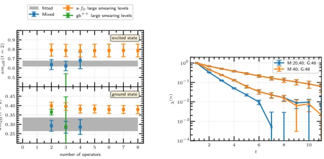
channel. The results of our calculations show that the enlarged variational basis leads to a more effective suppression of excited states contributions than using meson or glueball operators alone. Even the minimal choice of using only one meson and one glueball operator appears to be sufficient to extract the masses of the lowest two states in the scalar channel, see figure 6. Using more than one glueball or more than one meson operator does not improve this estimation, but provides better access to the excited states.

We therefore conclude that it is crucial to include both meson and glueball operators in the variational basis to reliably extract the ground state in the scalar channel.

Pseudoscalar 0

⁻⁺

channel. In this channel the estimation of masses does not improve

when the enlarged basis also includes glueball operators. The lowest two states can be

analysed sufficiently by using only meson operators, see figure 7, which means that the

glueball operators do not mix significantly with these states. This is in accord with the

observation that the entries in the off-diagonal blocks of the correlation matrix (5.1) are

zero (within rather large errors).

JHEP04(2019)150

0.5 0.6 0.7 0.8 0.9

ameff(t=2)

excited state fitted

Mixed

a-f₀large smearing levels gb⁺⁺large smearing levels

0 1 2 3 4 5 6 7 8

number of operators 0.25

0.30 0.35 0.40 0.45

ameff(t=2)

ground state

2 4 6 8 10

t 10⁻⁴

10⁻³ 10⁻² 10⁻¹ 10⁰

λ(n)

M:20,40; G:48 M:40; G:48

Figure 6. Left: the ground state and the first excited state of the 0⁺⁺-channel are accessible with the mixed basis of one meson and one glueball operator (blue). Adding further meson or glueball operators (blue) doesn’t improve the projection to the state. If only meson or only glueball operators are used (orange and green) excited contributions are not as effectively suppressed as compared to the mixed basis. Right: shown are the first three generalised eigenvalues λ⁽ⁿ⁾ of the GEVP in the 0⁺⁺-channel. In orange the results from using a mixed basis including one meson operator (smearing level 40) and one glueball operator (smearing level 48) are shown. Adding a further operator (mesonic, smearing level 20) to the mixed basis (also blue) doesn’t change the signal for the ground state and the first excited state, but a signal for a second excited state appears.

6 Supermultiplets

Using the methods explained above we have reanalysed the low-lying spectrum using the gauge configurations of our previous investigations [5]. The parameters of the configura- tions, on which the present investigation is based, are compiled in table 1.

The main improvements compared to the previous analysis are the use of the variational method in all three channels including glueball and meson operators in the 0

⁺⁺

channel (in previous investigations the variational method was only applied to the glueball analyses), the inclusion of the additional gluino-glue correlator C

γ4

(t), and the use of smeared gauge fields in the definition of Jacobi smearing. Due to these improvements, the contributions from higher states to the correlators and noise stemming from the Jacobi smearing are suppressed so that the effective mass plateaus can be estimated more reliably and smaller values of t

_min

can be used as the lower boundary of the fitting intervals. Consequently, we not only obtained more reliable and more precise estimates of the ground state masses, but we were also able to extract the masses of the first excited states, see figure 8.

For this investigation the full set of smearing levels under consideration consists of

the gluino-glue smearing levels N

APE

= (5, 15, . . . , 95) and the glueball smearing levels

N

_APE

= (4, 8, . . . , 64). Note, that in contrast to the analysis above, we used a more

conservative choice of smearing levels for the meson operators, namely N

_J

= (0, 3, 20, 40).

JHEP04(2019)150

0.6 0.8 1.0 1.2

ameff

excited states fitted

M:20,40

M:20,40; G:48

0 2 4 6 8 10

∆t 0.0

0.1 0.2 0.3 0.4 0.5 0.6

ameff

ground state

Figure 7. Effective masses in the 0⁻⁺-channel from a basis consisting of two mesonic operators (smearing levels 20 and 40) (blue), and a basis including an additional glueball operator (smearing level 48) (orange). The estimation of the ground state (lower panel) doesn’t change when the glueball operator is included. In the upper panel the first and second excited states of the mixed basis are shown (orange). They are of similar mass. Apparently one is the excited meson state (it aligns well with the excited state of the purely mesonic basis (blue)), and the other one is the glueball ground state.

It is preferable to use not more than four smearing levels in the 0

⁺⁺

channel since this assures that the eigenvalues of the GEVP are clearly separated in the region of the fit and additional operators do not reduce the contamination by excited states further. We therefore use combinations of two meson operators, e.g. N

_J

= (20, 40) and two glueball operators N

AP E

= (24, 48) in this channel. As explained above, including the glueball operator in the GEVP for the pseudoscalar channel does not improve the results, thus we have analysed the pseudoscalar meson a-η

⁰

and the glueball gb

⁻⁺

separately.

The fit intervals were determined at each ensemble individually based on the formation of effective mass plateaus and the stabilisation of the χ

²

/d.o.f of the fit. Using the mixed basis of glueball and meson operators allowed to include smaller time separations t

min

for the scalar channel compared to the a-η

⁰

. For the ensemble β = 1.9, κ = 0.14415 e. g.

we used t

_min

= 4 for the ground state and t

_min

= 3 for the excited state in the scalar channel whereas we used t

min

= 7 for ground and excited states of the a-η

⁰

. The errors were obtained statistically using the standard Jackknife procedure together with binning in order to properly take into account autocorrelations.

Due to the increased precision, we observed that in the chiral extrapolation the gluino-

glue mass deviated strongly from the assumed linear behaviour at the ensemble with the

largest adjoint pion mass at β = 1.9, κ = 0.1433. This resulted in a χ

²

/d.o.f ≈ 7.5 of the

linear fit to the chiral limit. We therefore neglected this data point for the gluino-glue. This

also contributes to the fact that the updated result for the gluino-glue mass is smaller than

JHEP04(2019)150

0.0 0.1 0.2 0.3 0.4 0.5

a/w₀ 0.0

0.5 1.0 1.5 2.0 2.5 3.0 3.5 4.0

w0m

gg⁽⁰⁾ a−η⁰⁽⁰⁾ 0⁺⁺⁽⁰⁾ gb⁻⁺⁽⁰⁾

0⁺⁺⁽¹⁾ a−η⁰⁽¹⁾ gg⁽¹⁾

Figure 8. Extrapolation to the continuum of the masses of the ground states and first excited states in the 0⁺⁺, 0⁻⁺ and 1/2⁺gluino-glue channels as explained in the text.

the one from our previous investigation. We also tested to use a second order polynomial instead, which gave a consistent result, but a slightly larger error.

The results for the masses, extrapolated to the chiral and to the continuum limit, are collected in table 2. The ground state masses, extrapolated to the continuum limit, agree quite well with each other within errors. Similarly to the ground states, the respective excited states also seem to form a mass degenerate supermultiplet of approximately three times the ground state mass. Interestingly the 0

⁻⁺

-glueball ground state and the excited state of the a-η

⁰

both have similar masses, but they appear as two independent states in the variational method which do not mix.

In the continuum limit, the two-particle decay threshold is well below the mass of the excited supermultiplet, meaning that decays into particles of the ground state are allowed. Since the operators presently used in the GEVP very likely have only small overlap with two-particle states, the full consideration of the effects of the strong decay channels would require to include in our variational basis also multi-particle operators, such as two glueballs with opposite momenta or a glueball and a gluino-glue. The resulting spectrum would be enlarged and would include also energy levels corresponding to two- particles interacting on a periodic box, fulfilling a quantisation condition that determines the resonance properties, such as the phase shift, of the excited supermultiplet [25]. Such calculations require, however, a very good precision that is out of reach in the singlet sectors within the current statistics. The excited energy levels within the single-hadron approximation are already a good estimate of the mass of the excited supermultiplet.

Compared to our previous investigations [5] the extracted ground state masses turn

out to be slightly smaller. The differences to the old results can be viewed as systematic

errors of the old results, which are now much better under control. This includes the

correct estimation of the fitting intervals and the exclusion of the gluino-glue mass at

β = 1.9, κ = 0.1433 in the chiral extrapolation.

JHEP04(2019)150

ID

β κ L³×T

#Conf

ama-π am⁽⁰⁾gg am⁽⁰⁾_a-η0 am⁽⁰⁾₀₊₊

A 1.6 0.15500 24

³×

48 1404 0.5757(41) 0.929(28) 0.626(13) 0.98(12) B 1.6 0.15700 24

³×

48 1324 0.3208(38) 0.730(16) 0.459(35) 0.540(75) C 1.6 0.15750 24

³×

48 1612 0.201(10) 0.633(31) 0.378(43) 0.458(68) D 1.75 0.14900 24

³×

48 9300 0.2380(14) 0.4043(88) 0.319(12) 0.463(15) E 1.75 0.14920 24

³×

48 9816 0.2026(18) 0.3709(90) 0.292(14) 0.395(24) F 1.75 0.14925 24

³×

48 6428 0.1968(20) 0.3714(69) 0.270(17) 0.330(30) G 1.75 0.14930 24

³×

48 10228 0.1897(26) 0.336(21) 0.265(20) 0.346(45) H 1.75 0.14940 32

³×

64 4956 0.1615(14) 0.3575(57) 0.258(23) 0.376(22) I 1.75 0.14950 32

³×

64 1692 0.1263(65) 0.3347(75) — 0.287(59) J 1.9 0.14330 32

³×

64 10176 0.28694(42) 0.3312(46) 0.3165(34) 0.336(24) K 1.9 0.14387 32

³×

64 10144 0.21330(92) 0.2842(25) 0.2447(58) 0.204(21) L 1.9 0.14415 32

³×

64 20704 0.17780(63) 0.2482(44) 0.2126(43) 0.288(20) M 1.9 0.14435 32

³×

64 10648 0.1498(32) 0.2255(72) 0.1978(50) 0.204(19) ID

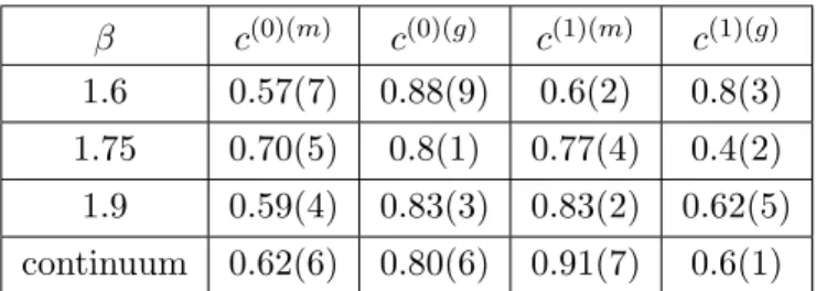
am⁽¹⁾gg am⁽¹⁾_a-η0 am⁽¹⁾₀++ c^(0)(g)₀++ c^(0)(m)₀++ c^(1)(g)₀++ c^(1)(m)₀++

A 1.31(11) 1.398(46) — 0.42(25) 0.71(13) — —

B 1.15(16) 1.077(60) 0.84(17) 0.82(22) 0.616(91) 0.44(11) 0.853(30)

C — — 0.65(25) 0.822(77) 0.586(74) 0.63(17) 0.68(13)

D 0.751(31) 0.724(24) 0.741(31) 0.602(71) 0.615(20) 0.787(75) 0.750(21)

E 0.756(23) 0.689(28) 0.715(44) 0.685(98) 0.604(35) 0.591(79) 0.784(24)

F 0.663(39) 0.764(21) 0.645(29) 0.718(67) 0.516(38) 0.523(44) 0.827(19)

G 0.621(44) 0.669(29) 0.688(58) 0.715(93) 0.654(39) 0.700(54) 0.732(30)

H 0.725(31) 0.688(35) 0.673(38) 0.650(84) 0.702(31) 0.70(10) 0.734(25)

I 0.695(75) — 0.69(10) 0.49(11) 0.686(55) 0.754(58) 0.685(76)

J 0.618(12) 0.708(15) 0.524(12) 0.920(13) 0.316(17) 0.266(34) 0.903(10)

K 0.560(10) 0.550(48) 0.451(16) 0.927(19) 0.352(27) 0.320(37) 0.901(11)

L 0.503(13) 0.497(27) 0.440(15) 0.797(37) 0.543(36) 0.499(40) 0.828(16)

M 0.505(14) 0.589(30) 0.435(19) 0.789(41) 0.577(45) 0.581(48) 0.793(31)

Table 1. Summary of the ensembles, masses of the lowest (superscript 0) and excited (superscript 1) states in lattice units, and mixing coefficient of the scalar channel. The ensembles have been presented in [4–6]. For consistency we use only the ensembles with one level of stout smearing. In some cases the data could not be extracted, because the fit intervals could not be determined reliably.

JHEP04(2019)150

β w

0

/a am

⁽⁰⁾₀++

am

⁽⁰⁾_a-η0

am

⁽⁰⁾gg

am

⁽¹⁾₀++

am

⁽¹⁾_a-η0

am

⁽¹⁾gg

am

⁽⁰⁾_gb−+

1.6 1.859(4) 0.37(7) 0.36(4) 0.62(2) 0.5(4) 0.93(9) 1.1(2) 1.01(1) 1.75 3.41(2) 0.25(4) 0.19(3) 0.312(9) 0.59(6) 0.68(5) 0.66(5) 0.7(1)

1.9 5.86(8) 0.17(3) 0.151(5) 0.17(1) 0.39(2) 0.46(3) 0.46(1) 0.50(5) cont. 1.1(2) 0.98(6) 0.93(7) 2.8(3) 3.1(2) 3.1(2) 3.4(4)

Table 2. Ground and excited state masses in lattice units extrapolated to the chiral limit (κ=κc), and the extrapolations to the continuum limit in units of the scalew₀. The subscript 0⁺⁺ denotes the result in the mixed channel, gg the gluino-glue, a-η⁰ the pseudoscalar meson and gb⁻⁺ the pseudoscalar glueball. The masses in the continuum limit are given asw0m. The quoted errors are statistical.

7 Mixing between glueballs and mesons

The numerical results of the extended variational approach indicate mixing between glue- ball and mesonic states. Such a mixing has been predicted in the literature on the structure of the lowest chiral supermultiplets [2, 3]. From the calculated correlation matrices we can get insights about the nature of the physical states with respect to their mesonic and glueball content.

From the eigenvectors ~ v

n

of the GEVP (3.2) the corresponding physical states |ni can be reconstructed and decomposed into a glueball contribution |φ

^(g)

i and a meson contribution |φ

^(m)

i:

|ni =

ng

X

i=1

v

_ni^(g)

O ˆ

_i^(g)

|Ωi +

nm

X

i=1

v

^(m)_ni

O ˆ

^(m)_i

|Ωi (7.1)

=

ng

X

i=1

v

_ni^(g)

|φ

^(g)_i

i +

nm

X

i=1

v

^(m)_ni

|φ

^(m)_i

i .

= |φ

^(g)_n

i + |φ

^(m)_n

i , (7.2)

where v

_ni^(g)

and v

_ni^(m)

are the components of the eigenvectors ~ v

_n

corresponding to the glueball operators O

^(g)_i

and the meson operators O

^(m)_i

, respectively, and |Ωi is the vacuum state.

Note that |ni , |φ

^(g)

i and |φ

^(m)

i are not normalised here.

The inner products c

_ni

.

= hφ

_i

|ni can be calculated as the vectors dual to the ~ v

_n

by means of [19]

X

i

v

_mi^∗

c

ni

= δ

mn

. (7.3)

So they are the row vectors of M

⁻¹

, where M is the matrix formed by the column vectors

~ v

n

. Let us denote c

^(g)_ni

= hφ

^(g)_i

|ni and c

^(m)_ni

= hφ

^(m)_i

|ni the restrictions of the c

ni

to the glueball and the meson components, respectively. The normalisations of the vectors can be obtained as

N

_n^(g)2

= hφ

^(g)_n

|φ

^(g)_n

i = X

ij

v

_ni^∗(g)

v

_nj^(g)

hφ

^(g)_i

|φ

^(g)_j

i = X

ij

v

^∗(g)_ni

v

^(g)_nj

X

k

c

^(g)_ki

c

^∗(g)_kj

(7.4)