Dynamical Systems and Nonlinear Ordinary Differential Equations

Dynamical Systems and Nonlinear Ordinary Differential Equations

Lecture Notes Christian Schmeiser¹

Contents

1. Introduction 1

2. Linear systems 7

2.1. Inhomogeneous linear ODE systems 9

3. Scalar ODEs – stability 10

4. Hyperbolic stationary points – linearization 11

5. Scalar ODEs – bifurcations 15

5.1. The fold 15

5.2. The transcritical bifurcation 16

5.3. The pitchfork bifurcation 16

5.4. The spruce budworm – the cusp bifurcation 17

6. Scalar iterated maps – bifurcations and chaos 18

7. Invariant regions – Lyapunov functions 20

8. Limit cycles 24

8.1. Multiple scales 24

8.2. The Poincar´e map 27

8.3. Relaxation oscillations 27

8.4. The Hopf bifurcation 29

8.5. The Poincar´e-Bendixson theorem 30

9. The Lorenz equations 33

10. Hamiltonian mechanics 36

Appendix 1 – second order Taylor remainders 43

Appendix 2 – Young’s inequality 44

References 44

1. Introduction

Most of the material for this course can also been found in the books [2, 4, 5], and we do not give detailed references to these in the following.

We consider models for the time evolution of systems, whose state can be described by a finite number of parameters.

• Thereforestates will always be points in Rⁿ,n∈N, thestate space.

• Time will be assumed to either evolvecontinuously or in discrete steps.

1Fakult¨at f¨ur Mathematik, Universit¨at Wien, Oskar-Morgenstern-Platz 1, 1090 Wien, Aus- tria. christian.schmeiser@univie.ac.at

1

• We shall also assume that the state at a certain time completely deter- mines all later states, and finally

• we assume that the environment for our system does not change with time.

Starting with the case of discrete time k ∈Z, the assumption that the state u_k ∈ Rⁿ at time k determines the state at time k+ 1 means that there is a map fk : Rⁿ → Rⁿ such that uk+1 = fk(uk). Since we also assume that the environment does not change with time, the rule for the time step from k to k+ 1, i.e. the map fk should not depend on k. Furthermore we consider the possibility that not all points in Rⁿ are admissible states, and postulate for f : M → M ⊂Rⁿ the evolution rule

u_k+1 =f(u_k), k∈Z. (1)

One particularforward trajectoryis fixed by prescribing an initial state u0 =u∈ M.

(2)

The choice of k= 0 as initial time is not essential by the independence of f on k. Since the forward trajectory is obviously given by

u_k=f^k(u) :=f◦ · · · ◦f

| {z }

ktimes

(u), k≥0,

we talk about iterated maps in this situation. If the map f is invertible, the initial state also determines the states at negative times, and the above formula can also be used fork <0 with the convention f^−k:= (f⁻¹)^k,k >0.

For continuous time we consider explicit first order autonomous systems of ordinary differential equations

˙

u(t) =f(u(t)) (3)

withu(t)∈Rⁿfort∈R,f :Rⁿ→Rⁿand ˙u:=du/dt. The differential equations areordinary, since the unknown functionu only depends on one variable. They areexplicit,since the derivatives of the components are given as functions of the state. Finally, autonomousmeans that f does not explicitly depend on t, which reflects the time independence of the environment.

Again we expect that prescribing the state at a certain time (w.l.o.g. chosen as t = 0) determines the subsequent evolution. We consider (3) subject to the initial condition

u(0) =u0. (4)

ThePicard-Lindel¨of Theorem shows that from t= 0 we can actually go forward and backward in time, at least a little:

Theorem 1. Letu0∈Rⁿand letf(u)be Lipschitz continuous in a neighborhood U ofu₀with values inRⁿ. Then there existsT >0and a uniqueu∈C¹((−T, T)) solving (3), (4), for −T < t < T. The existence time T only depends on U, on sup_U|f|, and on the Lipschitz constant of f in U.

The Picard theorem requires Lipschitz continuity off. In the following it will be convenient to assume even more regularity. In order to avoid technicalities concerning precise smoothness assumptions, we shall assume from now on

f ∈C^∞(Rⁿ)ⁿ, (5)

for the functions in both (1) and (3). This assumption will be used for the rest of the course, and it will not be repeated in each theorem.

The Picard-Lindel¨of theorem is a local existence theorem guaranteeing exis- tence only in a small enough time interval. The example

˙

u=u², u(0) = 1, (6)

with the explicit solution u(t) = (1−t)⁻¹ shows that in general no better result can be expected. We observe that the maximal existence interval (−∞,1) is open, and limt→1−|u(t)| = ∞ holds. The following result shows that ’nothing worse’ can happen.

Theorem 2. Let (5) hold and letu₀∈Rⁿ. Then the maximal existence interval I of the unique solution of (3), (4) is open, i.e. I = (a, b) with −∞ ≤ a <0<

b≤ ∞. In the cases a >−∞ or b <∞ we have

t→a+lim |u(t)|=∞ or, respectively, lim

t→b−|u(t)|=∞.

Remark 1. The Euclidian norm in Rⁿ is denoted by| · |and the scalar product by a dot, i.e. |u|² =u·u.

Proof: ForI =Rthere is nothing to prove. Therefore we first assumeb <∞. If limt→b−|y(t)|=∞does not hold, then there exists a sequencetn→b−, such that the sequenceu(t_n) is bounded and therefore it contains a convergent subsequence u(tnk)→u(by the Bolzano-Weierstrass theorem). Theorem 1 implies that for a neighborhoodU ofuthere existsT >0 such that for all ˜u∈U the solution of the initial value problem (3) subject tou(˜t) = ˜u exists in the interval (˜t−T,˜t+T).

Since (t_nk, u(t_nk))→(b, u), there existsn_k, such thatu(t_nk)∈U andb−t_nk < T. The solution can therefore be extended up to the timet_nk+T > bin contradiction to b being the right end of the existence interval. It is an obvious consequence that the existence interval is open atb.

The left end is treated analogously.

This result often helps in proving global existence of solutions, i.e. existence for all times. A useful auxiliary result is the Gronwall lemma:

Lemma 1. a) Let z: [0, T]→[0,∞) be continuous,λ, z₀ ≥0, and let z(t)≤z0+λ

Z t 0

z(s)ds , 0≤t≤T . Thenz(t)≤e^λtz₀, 0≤t≤T.

b) Let z : [0, T]→ [0,∞) be continuously differentiable, λ∈ R, z(0) =z0 ≥0,

and let

˙

z(t)≤λz(t), 0≤t≤T . Thenz(t)≤e^λtz0, 0≤t≤T.

Proof: a) The function

v(t) :=e^−λt Z t

0

z(s)ds satisfies

˙

v(t) =e^−λt

z(t)−λ Z t

0

z(s)ds

≤e^−λtz0. By integration we obtain

v(t)≤ z0

λ

1−e^−λt .

Sincez(t)≤z0+λe^λtv(t), the result follows. Note that λ≥0 is used in this last step.

b) The functionu(t) =e^−λtz(t) satisfies ˙u≤0 and, thus, u(t)≤u(0) =z0. The folllowing theorem is a typical global existence result.

Theorem 3. Let the assumptions of Theorem 2 be satisfied and let the right hand side f have at most linear growth, i.e. there exist λ, µ ≥ 0 such that

|f(u)| ≤λ|u|+µfor all u∈Rⁿ. Then for every u0 ∈Rⁿ the solution of (3), (4) exists for all times.

For every t∈R, u(t) depends Lipschitz continuously on the initial state u0. Proof: We prove existence for all t > 0. The proof for negative t is analogous aftert↔ −t.

The formulation of the initial value problem as integral equation u(t) =u0+

Z t 0

f(u(s))ds implies

|u(t)| ≤ |u₀|+ Z t

0

(λ|u(s)|+µ)ds

For λ = 0 this gives |u(t)| ≤ |u₀|+tµ. For λ > 0 we use the Gronwall lemma withz(t) =|u(t)|+µ/λand obtain

|u(t)| ≤e^λt|u₀|+µ λ

e^λt−1 .

In both cases|u(t)|cannot grow above all bounds in finite time. Thus the solution is global by Theorem 2.

For proving Lipschitz continuous dependence on the initial state, fix u₀ ∈Rⁿ and t ∈ R. Then the estimates above show that for initial states in a bounded neighborhood U of u0, the trajectories between times 0 and t lie in a bounded

set. Denote the Lipschitz constant of f in this set by L, choose v₀ ∈ U and let u(t), v(t) be the solutions of (3) with u(0) =u0, v(0) =v0. Then we have

|u(t)−v(t)| ≤ |u₀−v₀|+ Z t

0

|f(u(s))−f(v(s))|ds

≤ |u₀−v0|+L Z t

0

|u(s)−v(s)|ds ,

and, thus, by the Gronwall lemma,

|u(t)−v(t)| ≤e^Lt|u₀−v₀|.

Definition 1. Let M be a metric space (the state space or phase space) and let the set of times T be either R, [0,∞), Z, or N0. A deterministic dynamical system is a map T × M → M, (t, u₀)7→S_t(u₀), satisfying

(1) ∀u₀∈ M: S0(u0) =u0,

(2) ∀u₀∈ M,s, t∈ T: S_s+t(u₀) =S_s(S_t(u₀)), (3) ∀t∈ T: u0 7→St(u0) is continuous.

In the cases T = [0,∞) and T = N0, S_t is called a forward dynamical system;

for T = Z or T = N0 it is called a discrete dynamical system; and for T = R or T = [0,∞) it is called a continuous dynamical system. For fixed u0 ∈ M, the set {S_t(u0) : t∈ T } is called the trajectory through u0. The collection of all trajectories is called the phase portrait of the dynamical system.

Remark 2. Condition (1) just means thatu₀ is the initial state. Condition (2) is called the semigroup property, since it induces a semigroup structure for forward dynamical systems. For forward-and-backward dynamical systems (T = R or T =Z) it is actually a group structure with the inverse of St given by S−t.

Finally, condition (3) means continuous dependence on the initial state. For continuous dynamical systems one typically also expects continuity with respect to time.

Remark 3. Under the assumptions of Theorem 3, (3) defines a continuous dy- namical system on Rⁿ. Even if these assumptions are violated, a dynamical system might result from a reduction of the state space, e.g. the ODE in (6) defines a forward dynamical system onM= (−∞,0], but not on M=R.

The iteration (1) defines a discrete dynamical system on Rⁿ, whenever f is continuous. Discrete dynamical systems also result from the explicit Euler dis- cretization

u_k+1 =u_k+ ∆t f(u_k) of (3) with time step∆t.

In this course we deal with both discrete and continuous dynamical systems on finite dimensional state spaces. The solution operators of partial differen- tial equations and delay differential equations are typical examples for dynamical systems on infinite dimensional state spaces.

Remark 4. For continuous dynamical systems defined by ODEs, trajectories are either smooth curves or individual (stationary) points. By uniqueness of the so- lutions of initial value problems there is exactly one trajectory through each point.

Thus, the phase portrait provides a simple covering of the phase space. Know- ing this, the possible qualitative behaviors of trajectories are restricted, mainly by the dimension of the phase space. An application of these observations is the Poincar´e-Bendixson theorem (Section 8.5).

Dynamical systems theory (and therefore also this course) is mostly concerned with the investigation of the long-time behavior of trajectories and how it changes with varying initial state and in dependence of parameters. In this context, a basic object of study are steady states and their stability.

Definition 2. Let S_t, t∈ T, be a dynamical system on (M, d). Every u ∈ M satisfying St(u) =u for all t∈ T is called a stationary point or steady state. A steady state is called stable, if

∀ε >0 ∃δ >0 : d(u₀, u)< δ =⇒ d(S_t(u₀), u)< ε ∀t >0.

In words: Trajectories stay arbitrarily close to u, if they start close enough to it.

If u is not stable, it is called unstable.

A stable steady state u is called (locally) asymptotically stable, if

∃δ >0 : d(u0, u)< δ =⇒ lim

t→∞St(u0) =u . In words: Trajectories converge to u, if they start close enough to it.

An asymptotically stable steady state u is called globally asymptotically stable, if

∀u₀ ∈ M: lim

t→∞St(u0) =u . In words: All trajectories converge to u.

Remark 5. The steady states u of recursions u_k+1 =f(u_k) are the fixed points of f, i.e. u=f(u). The steady states u of ODEs u˙ =f(u) are the zeroes of f, i.e. f(u) = 0. Their stability properties are not seen quite as easily.

Definition 3. Let S_t, t ∈ T, be a dynamical system on (M, d). A set A⊂ M is called positively invariant, if

{S_t(u0) : u0∈A, t∈ T ∩(0,∞)} ⊂A

Definition 4. Let S_t, t∈ T, be a forward dynamical system on (M, d) and let u0 ∈ M. The omega limit ω(u0) of u0 is the set of all u ∈ M such that there exists a sequence{t_n}_n∈N⊂ T with limn→∞tn=∞, such thatStn(u0) =u.

Theorem 4. a) Omega limits are closed and positively invariant.

b) Let M = Rⁿ and let {S_t(u0) : t ∈ T ∩(0,∞)} be bounded. Then ω(u0) is nonempty and connected.

Proof: Proseminar.

2. Linear systems A special case of (1) is a linear homogeneous recursion

uk+1 =Auk

(7)

with a quadratic matrixA ∈R^n×n. In this case the solution of the initial value problem is given byu_k =A^ku0,k ≥0. With the help of a little linear algebra, this can be made more explicit. Particularly simple is the case of adiagonalizable matrix A, i.e. when there exists an invertible matrix R and a diagonal matrix Λ = diag(λ₁, . . . , λ_n), such that

A=RΛR⁻¹. (8)

In this case λ₁, . . . , λ_n are the eigenvalues of A and the columns ofR are corre- sponding eigenvectors. It is easily shown that

A^k=RΛ^kR⁻¹ =Rdiag

λ^k₁, . . . , λ^k_n

R⁻¹ (9)

holds. This implies that the solution can be written as a linear combination of eigenvectors of A with coefficients λ^k₁, . . . , λ^k_n. If for example |λ_j| < 1, j = 1, . . . , n, then the solution converges to zero as k → ∞ for arbitrary u₀. An alternative way to obtain the result is by diagonalizing the recursion. With the transformationu_k=Rv_k, i.e. representingu_k in terms of the basis given by the eigenvectors, we obtain the equivalent formulation

vk+1 = Λvk, i.e. vk+1,j =λjvk,j, j = 1, . . . , n , a decoupled system of scalar recursions with the obvious solution

v_k,j =λ^k_jv_0,j, k≥0, j= 1, . . . , n .

The diagonalized form also shows that for |λ_j| < 1, j = 1, . . . , n, u = 0 is the only steady state, which is globally asymptotically stable.

A decomposition of the form (8) always exists, but in general the matrix Λ is not diagonal, but contains Jordan blocks. The eigenvalues ofAare still important for the long-time behavior of solutions. We state the corresponding result without proof.

Theorem 5. Let |λ|<1 for all eigenvalues λ of A. Then for every initial state u0 the solution uk = A^ku0 of (7) converges to zero as k → ∞. If |λ| > 1 for at least one eigenvalue λ of A, then there exists u₀ ∈ Rⁿ such that u_k = A^ku₀ satisfieslimk→∞|u_k|=∞.

Remark 6. The theorem does not cover the case, where the spectral radius of A is equal to 1. In this case no general statement is possible. The behavior is determined by the Jordan block structure of possible multiple eigenvalues with modulus 1.

Now we turn to the continuous case and consider a linear homogeneous version of (3):

˙ u=Au (10)

again with a quadratic matrix A∈R^n×n. In this case the solution of the initial value problem is given byu(t) =e^Atu0, where the matrix exponential is defined by the power series

e^At:=

∞

X

j=0

(At)^j j! ,

whose convergence can be proven analogously to the convergence of the power series for the scalar exponential function. Also the proof of the semigroup prop- erty

e^A(t+s)=e^Ate^As, ∀s, t∈R,

is analogous to the case n= 1. The validity of the differential equation can be shown by term-by-term differentiation of the power series. For a diagonizable matrix A, the matrix exponential can be computed explicitly with the help of (9):

e^At =R e^ΛtR⁻¹ =Rdiag

e^λ1t, . . . , e^λnt R⁻¹.

Again the ODE system can be decoupled by the transformation u(t) = Rv(t).

We state a result on the long time behavior of trajectories also for possibly non- diagonizable matrices:

Lemma 2. Let Re(λ) <0 for all eigenvalues λof A. Then there exists λ <0, such that for every initial state u₀ the solution u(t) = e^Atu₀ of (10) satisfies

|u(t)| ≤e^λt|u₀|,t≥0. IfRe(λ)>0for at least one eigenvalue λofA, then there exists u₀ ∈Rⁿ such that u(t) =e^Atu₀ satisfies limt→∞|u(t)|=∞.

Remark 7. As in the previous theorem not all cases are covered. IfAhas eigen- values with non-positive real parts, then the Jordan block structure of multiple imaginary eigenvalues will be important for the stability properties of the steady state zero.

From our computations above it is easily seen that for diagonalizable matrices A, λcan be chosen as the maximum of the real parts of the eigenvalues of A. In the general case any value strictly bigger can be used.

Finally, let us consider the casen= 2, i.e.,

˙

v1 =λ1v1, v˙2=λ2v2, (11)

with the assumptionλ₁ <0< λ₂ on the eigenvalues. The positive and negative parts of the coordinate axes are trajectories, where thev1-axis is called thestable manifold, since it contains all initial values such that the solution converges to zero as t → ∞. Similarly, the v2-axis is called the unstable manifold, since it contains all initial values such that the solution converges to zero as t → −∞.

All other trajectories lie on curves with the equation

|v₁|^λ2|v₂|^−λ1 =c , c >0.

This can be seen by either differentiating this equation or by using the explicit solutions of (11). The trajectories have the qualitative behavior of hyperbolas filling the (v₁, v₂)-plane. As t→ ∞ they approach the unstable manifold, and as t→ −∞the stable manifold. This picture is qualitatively the same in the original (u₁, u₂)-plane. However, the stable und unstable manifolds are now spanned by the eigenvectors ofA.

2.1. Inhomogeneous linear ODE systems. For later reference we provide some results for inhomogeneous linear systems. Note that we permit time de- pendent inhomogeneities, i.e. non-autonomous equations. For a system of the form

˙

u=Au+h(t), (12)

with a constant matrix A∈R^n×n and a given inhomogeneity h(t) ∈Rⁿ, partic- ular solutions are given by thevariation of constants formula

u(t) = Z t

t0

e^A(t−s)h(s)ds ,

wheret₀ can be chosen arbitrarily. In particular, by the superposition principle, the solution of the initial value problem withu(0) =u0 is given by

u(t) =e^Atu₀+ Z t

0

e^A(t−s)h(s)ds . (13)

We now consider the situation, where h(t) is bounded in [0,∞), and look for bounded solutions of (12) in two different cases.

Lemma 3. Let h: [0,∞)→Rⁿ be continuous and bounded.

a) Let all eigenvalues of A have negative real parts. Then all solutions of (12) can be written in the form (13) and are bounded on[0,∞).

b) Let all eigenvalues of A have positive real parts. Then there is exactly one bounded solution of (12), given by

u(t) =− Z ∞

t

e^A(t−s)h(s)ds (14)

Proof: a) Clearly the set of all solutions can be parametrized by its state at t= 0 and, thus, all solutions are of the form (13). Withλ <0 from Lemma 2 we

have

|u(t)| ≤ e^λt|u₀|+ Z t

0

e^λ(t−s)|h(s)|ds≤ |u₀|+ sup

[0,∞)

|h|

Z t 0

e^λ(t−s)ds

≤ |u₀|+ 1

|λ| sup

[0,∞)

|h|.

b) Since now the eigenvalues of −A have negative real parts, Lemma 2 can be applied to this matrix with a corresponding λ < 0. This implies that for every u₀ 6= 0, the solution u_h(t) = e^Atu₀ of the initial value problem for the homogeneous equation cannot be bounded, since otherwise the estimate

|u₀|=|e^−Atu_h(t)| ≤e^λt sup

[0,∞)

|u_h|

would lead to a contradiction. Therefore it suffices to show that the solution given by (14) is bounded, since any other solution is obtained by adding an unbounded term of the forme^Atu₀.

|u(t)| ≤ Z ∞

t

e^λ(s−t)|h(s)|ds≤ 1

|λ| sup

[0,∞)

|h|.

3. Scalar ODEs – stability

An ODE of the form ˙u=f(u) withf :R→Rcan in principle be solved: The solution subject to the initial conditionu(0) =u₀ is implicitly given by

Z u(t) u0

dη f(η) =t .

Typically, the qualitative behavior of solutions is not obvious from this formula.

On the other hand, it can easily be seen directly fromf. Because of its continuity the state space (i.e. the u-axis) is the union of the zeroes off on the one hand, and open intervals where f is either positive or negative, on the other hand.

Zeroes u0 of f are steady states, since the solution of the initial value problem withu(0) =u0 is the constant u(t) =u0,t∈R.

Suppose on the other hand that f is positive between two zeroes u₁, u₂ and u1 < u0 < u2. Then the solution starting at u0 exists for all time and satisfies

t→−∞lim u(t) =u₁, lim

t→∞u(t) =u₂.

As a third case letf be positive everywhere to the right of the zero u₁, then for u₀ > u₁,

t→−∞lim u(t) =u1, lim

t→Tu(t) =∞,

whereT ≤ ∞is the right end of the existence interval. For all other possible cases similar statements hold. In particular, trajectories either converge as t → ±∞

or they tend to∞ or−∞. The proofs are easy and left to the reader.

The stability of steady states is easily seen. If a steady stateu is isolated, and the sign of f changes at u from positive to negative, then u is asymptotically stable. Isolated steady states with any other behavior of f in the neighborhood are unstable. If a steady state lies in the interior of an interval, wheref vanishes, then the steady state is stable, but not asymptotically stable.

Simple examples:

• u˙ = 0 : Every u ∈ R is a stable, but not asymptotically stable, steady state.

• u˙ =−u:u= 0 is a globally asymptotically stable steady state.

• u˙ =u, ˙u=±u² :u= 0 is an unstable steady state.

• u˙ =u³−u:u= 0 is a locally asymptotically stable steady state. u=±1 are unstable steady states.

4. Hyperbolic stationary points – linearization

Although usually not really necessary for scalar equations, it is a reasonable idea to study local stability properties by using local approximations of f, i.e.

Taylor polynomials. If in the ODE the function f is approximated by its first order Taylor polynomial around a steady stateu,

f(u)≈f(u) +f⁰(u)(u−u) =f⁰(u)(u−u), the resulting linear ODE forv≈u−u,

˙

v=f⁰(u)v , (15)

is called thelinearization of (3) atu. Obviously, the steady state v = 0 of (15) is asymptotically stable for f⁰(u) < 0, stable for f⁰(u) = 0, and unstable for f⁰(u)>0. Consequences for the underlying nonlinear ODE are easily seen:

Theorem 6. Let n= 1 and let u be a steady state of (3). If f⁰(u) <0, then u is locally asymptotically stable. If f⁰(u)>0, then u is unstable.

The simple proof is left to the reader. There is no conclusion for f⁰(u) = 0, because in this case the local behavior of f around u, and therefore also its stability properties, depend on higher order terms in the Taylor expansion. The examples ˙u = 0, ˙u = ±u³ share the linearization at u = 0 with f⁰(u) = 0, but not the stability properties.

The linearization approach can also be used for systems. Then the linearized equation reads ˙v=Df(u)v(the generalization of (15)) with the Jacobian matrix Df(u). We generalize the assumptions of Theorem 6 to higher dimensions.

Definition 5. Let n ≥ 1 and let u be a steady state of (3). Then u is called hyperbolic, if Re(λ)6= 0 for all eigenvalues λ of the JacobianDf(u).

The term hyperbolic can be motivated by the two-dimensional linear example in Section 2. We shall use the fact that for hyperbolic steady states the Jacobian can be block diagonalized, i.e.

Df(u) =RΛR⁻¹, with Λ =

Λ− 0 0 Λ+

, R= (R−, R₊), (16)

where Λ− ∈R^k×k, 0≤k≤n, has only eigenvalues with negative real parts, and Λ+ ∈ R(n−k)×(n−k) has only eigenvalues with positive real parts. The columns ofR−∈R^n×k are generalized eigenvectors corresponding to the eigenvalues with negative real parts, and the columns ofR₊∈R^n×(n−k) are generalized eigenvec- tors corresponding to the eigenvalues with positive real parts.

Theorem 7. (Stable manifold theorem)Let u∈Rⁿ be an hyperbolic steady state of the dynamical systemS_t generated by (3). Then there is a neighborhood U ⊂Rⁿ of u, such that

M_s[u] :={u₀ ∈U : S_t(u₀)∈U, t≥0}

is ak-dimensional (referring to the diagonalization (16)) manifold in Rⁿ, called the stable manifold of u. For allu0∈ M_s[u],

|S_t(u0)−u0| ≤c e^λ−t, t≥0, (17)

wherec≥0 andλ− <0is the constantλfor the matrixΛ− from Lemma 2. The tangent space of M_s[u]at u is spanned by the columns of R− from (16), i.e. by the eigenvectors corresponding to eigenvalues of Df(u) with negative real parts.

Analogously, the set

M_u[u] :={u₀ ∈U : S_t(u₀)∈U, t≤0}

is a (n−k)-dimensional manifold in Rⁿ, called the unstable manifold of u. For allu0∈ M_s[u],

|S_t(u0)−u0| ≤c e^λ+t, t≤0,

where c ≥ 0 and −λ₊ < 0 is the constant λ for the matrix −Λ₊. The tangent space of M_u[u] atu is spanned by the columns of R₊.

Remark 8. Obviously, hyperbolic steady states are either locally asymptotically stable (k = n) or unstable. For non-hyperbolic steady states, the linearization does not contain sufficient information for a complete characterization of the local behaviour. In particular, if all eigenvalues have non-positive real parts with at least one eigenvalue on the imaginary axis, then there is no conclusion concerning the stability properties of the steady state.

Proof: The right hand side of (3) can be written as f(u) = Df(u)(u−u) + R r(R⁻¹(u−u)) with the second order remainder term, which we have chosen to write in this form with the matrixR from (16). We decouple increasing and decreasing modes by the transformationu(t) =u+Rv(t), and obtain

˙

v= Λv+r(v).

With the notationv= (v−, v₊),r = (r−, r₊), according to the block structure of Λ, this can be written as

˙

v−= Λ−v−+r−(v), v˙₊= Λ₊v₊+r₊(v).

Letu0 be in the setM_s[u]. Then St(u0), and therefore alsov(t) =R⁻¹(St(u0)− u), and consequentially r(v(t)) are bounded for t ≥ 0. Thus we can use the results of Lemma 3 to obtain

v−(t) = e^Λ−tp+ Z t

0

e^Λ−(t−s)r−(v(s))ds , (18)

v₊(t) = − Z ∞

t

e^Λ+(t−s)r₊(v(s))ds , (19)

for some p ∈R^k. In the following we shall prove that for given small enough p the integral equation problem (18), (19) has a unique solution. Therefore v₊(0) is determined as a function ofp=v−(0), and the stable manifold in thev-space is thus given as the graph of a function from R^k toR^n−k.

In order to prove the decay estimate (17) at the same time, we set v(t) = e^λ−tw(t) in (18), (19):

w−(t) = e^{(Λ−−λ−)t}p+e^−λ−t Z t

0

e^Λ−(t−s)r−(e^λ−sw(s))ds , (20)

w₊(t) = −e^−λ−t Z ∞

t

e^Λ+(t−s)r₊(e^λ−sw(s))ds . (21)

We shall use the Banach fixed point theorem for w in the space C_B([0,∞))ⁿ (bounded continuous functions), noting that (20), (21) has the fixed point form w=F(w). Actually we shall restrict to a ball

B_δ:={w∈CB([0,∞))ⁿ: kwk∞< δ},

where k · k_∞ denotes the supremum norm on [0,∞). We shall always assume (p,0)∈ B_δ/2.

Our first claim is that

F : B_δ→ B_δ forδ small enough.

(22)

Since by Lemma 2,|e^Λ−tu0| ≤e^λ−t|u₀|,t≥0, and|e^Λ+tu0| ≤e^λ+t|u₀|,t≤0, we have for w∈ B_δ,

|F(w)−(t)| ≤ |v₋(0)|+ Z t

0

e^−λ−s|r₋(e^λ−sw(s))|ds≤ δ 2+δ²L

Z t 0

e^λ−sds

≤ δ

2 + δ²L

|λ₋|,

|F(w)₊(t)| ≤ e^{(λ+−λ−)t} Z ∞

t

e^−λ+s|r₊(e^λ−sw(s))|ds

≤ δ²L e^{(λ+−λ−)t} Z ∞

t

e^{(2λ−−λ+)s}ds≤ δ²L λ₊−2λ−

,

where we have used the Lipschitz continuity estimate (52) from the Appendix.

After summing these inequalities, (22) is obvious. It remains to prove that, again forδ small enough, F is a contraction: For w₁, w₂∈ B_δ,

|F(w₁)−(t)−F(w₂)−(t)| ≤ Z t

0

e^−λ−s|r₋(e^λ−sw₁(s))−r−(e^λ−sw₂(s))|ds

≤ δL Z t

0

e^λ−s|w₁(s)−w₂(s)|ds≤ δL

|λ−|kw₁−w₂k_∞,

|F(w₁)+(t)−F(w2)+(t)| ≤ δLkw₁−w2k∞e^{(λ+−λ−)t} Z ∞

t

e^{(2λ−−λ+)s}ds

≤ δL

|λ₊−2λ−|kw₁−w₂k_∞.

Again, summing the inequalities immediately implies the contraction property for δ small enough. This implies that for each small enough p there exists a unique (in a small ball) solution of (18), (19) satisfying (17). Thus, u0(p) = u+Rv(0;p) is a parametrization ofM_s[u] with parameterp∈R^k. An extension of the Banach fixed point theorem for problems with parameters implies that the solution depends smoothly on p.

It remains to determine the tangent space at u0 =u, which obviously is ob- tained with p = 0, whence (18), (19) has the solution v = 0. The function zj(t) =∂pjv(t)|_p=0 satisfies

(z_j)−(t) =e^Λ−te_j, (z_j)₊(t) = 0,

with the jth canonical basis vector e_j ∈ R^k, since the derivative of the second order remainder at zero vanishes. Thus, ∂pju0 |_p=0= Rj, the jth column of R, 1 ≤ j ≤ k. This shows that the tangent space has maximal dimension k, and M_s[u] is really ak-dimensional manifold.

After time reversal, the proof for the unstable manifold is the same.

The stable manifold theorem tells us that essential properties of the dynam- ics near hyperbolic fixed points are shared by the full nonlinear system and its linearization. An even stronger result in this direction, which we state without proof (which can be found in e.g. [5]), is the Hartman-Grobman theorem. It says that close to an hyperbolic fixed point the dynamics of the nonlinear system and of the linearization are the same up to a diffeomorphism (differentiable and one-to-one with differentiable inverse):

Theorem 8. (Hartman-Grobman)Letu∈Rⁿbe an hyperbolic steady state of (3). Then there is a diffeomorphism ϕ: U →V between a neighborhoodU ⊂Rⁿ of u and a neighborhood V ⊂ Rⁿ of the origin, such that Dϕ(u)f(u) = Λϕ(u) (with Λ from (16)), i.e. if u(t)∈U solves (3), then v(t) :=ϕ(u(t)) solves

˙

v=Dϕ(u) ˙u=Dϕ(u)f(u) = Λv .

We shall be interested in dynamical systems containingparameters. For ordi- nary differential equations, this means to consider systems of the form

˙

u=f(u, r) withr ∈R^l, (23)

and to study the dependence of the long-time behavior on the parameters. In the following, we shall always assume smoothness off, not only with respect to the stateu, but also with respect to the parametersr:

f ∈C^∞(Rⁿ×R^l)ⁿ. (24)

The parameter dependence motivates a second stability concept:

A property of (23) is called structurally stable (or generic), if it is preserved under small parameter changes.

Theorem 9. The existence of an hyperbolic steady state is structurally stable:

Let, for r =r0 ∈R^l, (23) have an hyperbolic steady state u0 ∈ Rⁿ. Then there exists a neighborhoodR⊂R^l of r₀, such that (23) has an hyperbolic steady state u(r) for every r ∈R with u(r0) =u0 and u ∈C^∞(R)ⁿ. The dimensions of the stable and unstable manifolds through u(r) do not depend on r∈R.

Proof: (outline)Since the hyperbolicity ofu0implies thatDuf(u0, r0) is invert- ible, the existence and smoothness ofuare a consequence of the implicit function theorem. Since zeroes of polynomials depend continuously on parameters [1], the signs of the real parts of the eigenvalues ofDuf(u(r), r) do not change close to r=r₀.

5. Scalar ODEs – bifurcations

As we have seen in Section 3 one dimensional dynamics seems rather boring.

Trajectories either converge to steady states or they take off towards±∞. In this section we investigate how the long-time behavior might change with a varying parameter. Therefore we consider (23) with n=l= 1. Since hyperbolic steady states are structurally stable, qualitative changes in the dynamic behavior (called bifurcations) require the occurrence of a non-hyperbolic steady state. In the following we assume that for the critical parameter valuesr = 0 the originu= 0 is a non-hyperbolic steady state, i.e.

f(0,0) =∂_uf(0,0) = 0. (25)

5.1. The fold. With the assumption (25), the Taylor expansion of f around u=r= 0 has the form

f(u, r) =a₀₁r+a₂₀u²+a₁₁ru+a₀₂r²+O(u³+r³). (26)

A simple example is

˙

u=r+u². (27)

The bifurcation occurring at r = 0 can be described as follows: For r < 0 there are two hyperbolic steady states, the unstable point u = √

−r and the

asymptotically stable point u=−√

−r. They merge atr= 0, and for positiver there is no stationary point.

In the literature this bifurcation is called the fold or the saddle-node bifurac- tion. It is not as special as it seems. Consider the general case (26) in the generic situation, where the first two coefficientsa₀₁ anda₂₀are different from zero. We claim that there is a transformation taking (23) with (26) to (27). Note the similarity to the Hartman-Grobman Theorem 8.

We shall not provide a full proof, but some formal arguments for this result.

As a first step, we replaceu by _a^u

20 and r by _a ^r

01a20. This transforms (26) to

˙

u=r+u²+a₁₁ru+a₀₂r²+O(u³+r³),

after renaming coefficients. A heuristic argument is that the termsa₁₁ru,a₀₂r², and O(r³) are small compared to r and that O(u³) is small compared to u², and that all these terms can therefore be neglected. We shall show how the two quadratic terms can be eliminated by the close-to-identity transformation

r=R+bR², u=U+cU². (28)

It requires some computation to obtain the transformed equation U˙ =R+U²+ (a₁₁−2c)RU+ (a₀₂+b)R²+O(U³+R³).

The choiceb=−a₀₂,c=a11/2 produces (27) up to a third order remainder. By replacing the quadratic polynomials on the right hand sides of (28) by complete Taylor expansions, the form (27) can be produced exactly (see, e.g., [2]).

This means that a fold occurs, whenever we have the form (26) witha₀₁, a₂₀6=

0. Equation (27) is called thenormal form of the fold. In the following we shall present the normal forms of other bifurcations without discussing the transfor- mation to the normal form each time.

5.2. The transcritical bifurcation. The fold isthegeneric bifurcation in one- dimensional dynamical systems. Other types of bifurcations occur in systems with special properties, which do not change with parameter variations. A typical property of this kind is an always existing special steady state, w.l.o.g. u= 0. In this case, the coefficientsa₀₁ and a₀₂ in (26) vanish. Assuming apart from that a generic situation, meansa20, a116= 0. A corresponding normal form is

˙

u=ru−u².

This defines the transcritical bifurcation with the following properties: For all values of r we have the steady states u = 0 and u = r. For r < 0, u = 0 is asymptotically stable and u = r is unstable, and vice versa for r > 0. At the bifurcation an exchange of stability takes place.

5.3. The pitchfork bifurcation. Sometimessymmetriesare present in dynam- ical systems and invariant under parameter changes. A simple example is a re- flection symmetry, where the system does not change, when replacingu by −u.

This leads to the assumption that f is an odd function of u. The consequential normal form is

˙

u=ru−u³,

exhibiting the pitchfork bifurcation: For r < 0 there is one steady state u = 0, which is asymptotically stable. For positive r the stability of u = 0 is lost and transferred to the two new steady states u = ±√

r. It is a consequence of the symmetry that for each steady state its reflection also is a steady state with the same stability properties.

5.4. The spruce budworm – the cusp bifurcation. The spruce budworm is a north American tree pest, posing a recurrent threat for forests of conifer trees.

Sometimes sudden dramatic increases in the budworm population are observed without big changes in the environment.

We shall describe a budworm population by a continuous dynamical system.

LetN(τ) be a measure for the size of the population at time τ. The equation dN

dτ =RN

1− N K

− BN² A²+N²

is a typical model of population dynamics. The factor R(1−N/K) is the dif- ference between the birth rate and the death rate. This is a standard model for competition. The second term on the right hand side describes the loss caused by natural enimies: birds in the case of the budworm, eating the budworm with a maximal rateB. The dependence on the population size N has the following interpretation: If the population is significantly smaller than the thresholdA, it does not pay for the birds to look for the budworms, and they mainly look for other kinds of food. Above the critical size A the budworms become attractive as food and are eaten at a rate close toB.

We start by introducing the nondimensional variables t:= τ

A/B, u(t) := N(tA/B)

A .

The equation foru reads

˙

u=ru 1−u

k

− u² 1 +u²

with thedimensionless parametersr =RA/B undk=K/A. Note that we have reduced the number of parameters from four to two. This greatly simplifies the analysis of the qualitative properties of the model.

Apart from the trivial steady stateu= 0 (always unstable, i.e. the budworms do not die out), there are other steady states satisfying

r

1−u k

= u

1 +u² .

Depending on the values ofrandk, this equation has 1–3 positive solutions. The regions with different numbers of steady states are separated by folds, occurring

when the derivatives of the left and right hand sides coincide. This requirement leads to the relations

r= 2u³

(1 +u²)², k= 2u³

u²−1 with u >1,

which can be seen as parametrization (with parameteru) of a curve in the (r, k)- plane. This curve has a cusp at the point (r₀, k₀) = (3√

3/8,3√

3) (foru₀=√ 3).

Three positive steady states exist between the two branches of the curve, and one in the rest of the (r, k)-plane. In the latter case, the steady state is asymptotically stable, whereas in the former two of the steady states are asymptotically stable with an unstable steady state in between.

Now the following scenario is possible for the budworm population: Let r be fixed with a value between 1/2 and 3√

3/8, and let k increase slowly (e.g. by the growth of the trees). This gives a straight line in the r(, k)-plane, which twice intersects the bifurcation curve. Before the first intersection there exists a unique stable equilibrium with small values of the budworm population. At the first crossing of the bifurcation curve, a large stable and a middle sized unstable equilibrium are created, but the small equilibrium remains stable and the pop- ulation remains at this low level. A dramatic change happens, however, at the second crossing of the bifurcation curve. Now the small stable and the medium sized unstable equilibrium disappear, and only the large stable equilibrium is left.

A fast growth of the population has to be expected.

This qualitative behavior is already present in small neighborhoods of the cusp point (r₀, k₀). A normal form of this so calledcusp bifurcation is given by

˙

u=r+ku+u³,

where (r, k, u) now has to be interpreted as the deviation from (r₀, k₀, u₀). The cusp bifurcation needs two parameters, whence it is called acodimension 2 bifur- cation,in contrast to the bifurcations dealt with above, which are of codimension 1.

6. Scalar iterated maps – bifurcations and chaos

Instead of a general discussion, we only treat one (actually the most famous) example, the logistic map:

u_k+1=ru_k(1−u_k), (29)

with the parameter r > 0. This can be interpreted as a model for population dynamics, if we restrict to values of uk between 0 and 1, such that uk+1 is nonnegative. In order to remain in the interval [0,1], we also have to assume r≤4. Thus, for the rest of this section we assume

0< r≤4, 0≤u0≤1, guaranteeing 0≤u_k≤1 for allk≥0.

It turns out that the long-time behavior strongly depends onr. The situation is easy forr <1: Since obviouslyu_k+1≤ru_k,u_k≤r^ku0follows by induction. All solutions converge to zero and the population dies out. In terms of the vocabulary of dynamical systems: Zero is the only steady state in the state spaceM= [0,1], and it is globally asymptotically stable.

More generally, the stability of a steady stateu=f(u) of the discrete dynam- ical system

uk+1 =f(uk) (30)

can be examined by linearization: The recursion v_k+1=f⁰(u)v_k,

the linearization of (30) at u, can be expected to approximate small values of v_k=u_k−u.

Theorem 10. Let f : [a, b] → [a, b] be twice continuously differentiable. The steady stateuof (30) is asymptotically stable, if|f⁰(u)|<1. In the case|f⁰(u)|>

1 it is unstable.

Proof: By the Taylor formula, the exact equation forv_k can be written as v_k+1 =f(u_k)−f(u) =f⁰(u)v_k+f⁰⁰(˜u_k)v_k²/2,

(31)

with ˜u_k ∈[a, b], and therefore

|v_k+1| ≤ |v_k| |f⁰(u)|+|v_k|M/2 ,

with |f⁰⁰(˜u_k)| ≤ M. For |f⁰(u)| < 1 we choose δ := (1− |f⁰(u)|)/M, r :=

(1 +|f⁰(u)|)/2 <1, and |v₀| ≤δ. Induction implies |v_k| ≤ r^kδ →0, proving the first statement of the theorem.

For|f⁰(u)|>1 we start again from (31) and deduce

|v_k+1| ≥ |v_k|(|f⁰(u)| − |v_k|M/2).

For|v_k| ≤ε:= (|f⁰(u)| −1)/M and r:= (1 +|f⁰(u)|)/2>1 we then have

|v_k+1| ≥r|v_k|,

meaning that for arbitrarily small|v₀| we reach |v_k|> ε in finitely many steps, implying instability of u.

Remark 9. In the critical case|f⁰(u)|= 1 every stability behavior is possible, as can be seen from the examplesuk+1=uk(1±uk) and uk+1 =uk with u= 0.

Returning to (29), we see that for increasing values of r the steady state u1 = 0 loses its stability at the bifurcation point r = 1. For r > 1 there is a second steady stateu₂ = 1−1/rwhich, byf⁰(u₂) = 2−ris asymptotically stable for 1< r <3. This is the occurrence of a transcritical bifurcation in a discrete dynamical system.

At the second bifurcation poinitr= 3 alsou₂ loses its stability. The behavior of the dynamical system for r > 3 can be understood by analysing z_k := u_2k, k≥0, which solves the recursion

z_k+1 =ru_2k+1(1−u_2k+1) =r²z_k(1−z_k)(1−rz_k(1−z_k)). (32)

Besides u₁ = 0 and u₂ = 1−1/r this recursion has two more steady states for r >3:

z_3,4= 1 2r

1 +r±p

(r+ 1)(r−3) .

It is easily seen that z₃ = f(z₄) and z₄ = f(z₃), i.e. the poiints z₃ and z₄ constitute aperiodic orbit with period 2 of the original recursion (29). Note that the periodic orbit is created at the steady stateu₂:

u2=z3 =z4 = 2

3 forr= 3.

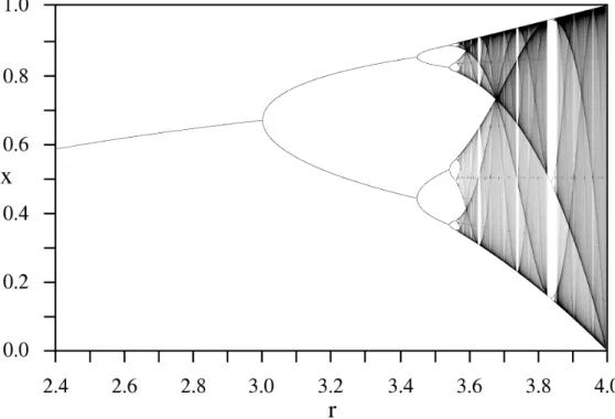
Further results, described in the following, are not as easy to verify. It can be shown that z3 and z4 are asymptotically stable steady states of (32) for r > 3 close to 3. This implies asymptotic stability of the periodic orbit of (29), where the meaning of this statement should be clear without precise definition. This stability gets lost at the further bifurcation point r = r₄. The bifurcation is similar to the one at r = 3: From each of the steady states z3 and z4 of f ◦f bifurcate two new steady states of the four times iterated map f ◦f ◦f ◦f, which together form a periodic orbit of period 4 of (29). This is called aperiod doubling bifurcation. For increasing values of r there is a sequence of period doubling bifurcations at the bifurcation pointsr₄ < r₈< r₁₆< . . .This sequence converges to the value rc < 4. Typical trajectories of (29) with r > rc show appearantly completely irregular behavior. This sensational discovery (of the 1970s) has been termeddeterministic chaos. As can be seen from the bifurcation diagram (Fig. 1), we actually have still not told the whole story.

We conclude by considering the special caser= 4, when the recursion can be solved explicitly with the ansatz u_k = sin²ϕ_k, leading to ϕ_k+1 = 2ϕ_k and the explicit solution

uk = sin²(2^kϕ0) withϕ0 = arcsin(√ u0).

Note that there exist periodic trajectories with arbitrary period p (e.g. for ϕ0 = π/(2^p −1)), but for most initital values the behavior looks completely unpredictable, e.g. wheneverϕ₀/π /∈Q.

7. Invariant regions – Lyapunov functions

Definition 6. A set M ⊂ Rⁿ is called positively invariant for (3), if every solution u of (3) withu(0)∈M satisfies u(t)∈M for all t≥0.

Lemma 4. LetΩ⊂Rⁿ be a bounded domain with smooth boundary∂Ω, letν(u), u∈∂Ω, denote the unit outward normal, and let ν(u)·f(u) ≤0, u∈∂Ω. Then the closure Ω is positively invariant for (3).

Figure 1. The bifurcation diagram of the logistic map

Proof: First we consider the stronger assumption ν(u)·f(u) <0, u ∈ ∂Ω. In this case every trajectory starting on ∂Ω enters Ω and, consequentially, cannot leave Ω. Since Ω is bounded, this also implies existence of trajectories for all t≥0 by Theorem 2.

Now we return to the assumptions of the Theorem and define fε(u) =f(u)−εν(u), ε >0,

which satisfies ν ·f_ε ≤ −ε < 0. Therefore, the solution u_ε of the initial value problem ˙uε=fε(uε),uε(0) =u0∈Ω, remains in Ω for all times and, in particular, for an arbitrary T > 0, uε(T) ∈ Ω holds. Thus uε : [0, T] → Rⁿ is bounded uniformly in ε as ε→ 0. By the differential equation, the same is true for ˙u_ε. As a consequence of the Arzela-Ascoli Theorem, there exists a sequence εn →0 such thatu_εn →u uniformly on [0, T]. Therefore we can pass to the limit ε→0 in the integrated version

uε(t) =u0+ Z _t

0

f(uε(s))−εν(uε(s)) ds

of the problem foru_ε with the result u(t) =u₀+

Z t 0

f(u(s))ds .

Since this is equivalent to the problem ˙u = f(u), u(0) = u0, and the uniform convergenceuε→u impliesu(T)∈Ω, the proof is complete.

In the following we use the notationB_r(u₀) ={u∈Rⁿ: |u−u₀|< r}for open balls inRⁿ.

Definition 7. a) Let u0 ∈ Rⁿ be a steady state of (3) and let V : Rⁿ → R satisfy V(u₀) = 0, V locally positive definite, i.e. ∃r >0 such thatV(u)>0 for u∈Br(u0)\ {u₀}, and ∇V(u)·f(u)≤0 locally, i.e. for u∈Br(u0). Then V is called a Lyapunov function for(f, u₀).

b) For a Lyapunov function V we define for δ > 0 the sublevel set S_δ as the connected component of {u: V(u)≤δ} containingu0.

Lemma 5. Let V be a Lyapunov function for(f, u0).

a) For every small enough r >0 exists δ >0, such that S_δ⊂B_r(u₀).

b) For every δ >0 exists r >0, such that Br(u0)⊂Sδ. Proof: a) For givenr >0 chooseδ >0 such that

δ < min

∂Br(u0)V ,

where the right hand side is positive for small enough r because of the local definiteness of V. This implies S_δ ∩∂Br(u0) = {}. Since also u0 ∈ S_δ, the connectedness ofS_δ implies that it cannot contain any points outside ofB_r(u₀).

b) For given δ >0 we define the closed level set Σ_δ := {u∈Rⁿ : V(u) =δ}. If it is empty, the result holds with arbitraryr >0. Otherwise let

r:= min

Σδ

|u−u0|>0.

For u ∈ B_r(u₀), V(u) > δ cannot hold since then, by the continuity of V and by V(u0) = 0,V would have to take the value δ somewhere on the straight line segment betweenu₀ and u, in contradiction to the definition of r.

Lemma 6. Let V be a Lyapunov function for (f, u₀). Then for small enough δ, sublevel sets Sδ are positively invariant for (3).

Proof: By Lemma 5 a), S_δ is bounded for δ small enough. For solutions u of (3), the Lyapunov function is non-increasing along the solution:

d

dtV(u(t)) =∇V(u(t)·f(u(t))≤0, which implies the result.

Theorem 11. Let V be a Lyapunov function for(f, u₀).

a) Thenu0 is stable.

b) If furthermore −∇V ·f is locally positive definite, then u₀ is asymptotically stable.

c) IfV and−∇V·f are globally positive definite, and all sublevel sets are bounded, thenu0 is globally asymptotically stable.

Proof: a) Letε >0 and let δ be as in Lemma 5 a) withr =ε. For this δ letr be as in Lemma 5 b). Then foru(0)∈B_r(u₀)⊂S_δ we have u(t)∈S_δ⊂B_ε(u₀).

b) Let δ >0 be small enough such thatSδ is bounded and positively invariant, and letube a solution of (3) with u(0)∈S_δ. Then by monotonicity there exists δ∗ := limt→∞V(u(t)). Assume δ∗ > 0. Then every accumulation point u∗ of u(t) satisfies u∗ ∈ Σ_δ∗ and therefore u(t) ∈/ Br(u0) for some r >0, t≥T. This however implies

lim sup

t→∞

d

dtV(u(t))

= lim sup

t→∞

∇V(u(t))·f(u(t))<0,

a contradiction to the convergence ofV(u(t)). Thusδ∗ = 0 with the consequence thatu0 is the only accumulation point of u(t).

c) Everyu(0) lies in some sublevel set. The rest of the proof is as in b).

Example 1. a) u¨+ sinu= 0. V(u) = 1−cosu+ ˙u²/2.

b) The equation u¨+ sinu+ku˙ = 0 for a pendulum with friction is equivalent to the first order system

˙

u=v , v˙=−sinu−kv .

The origin is a steady state which can be shown to be asymptotically stable for k >0by linearization. A Lyapunov function is given by the total energy V(u) = 1−cosu+v²/2. However, the decay

V˙ =−kv² is not negative definite.

c) Still for the damped pendulum, we tryV_ε(u) = 1−cosu+v²/2+εuv,0< ε1.

Using the second order Taylor polynomial of the cosine and Young’s inequality (see Appendix 2) withp=q = 2, γ = 1, we obtain

Vε(u)≈ u²+v²

2 +εuv ≥ 1−ε

2 (u²+v²),

showing the local definiteness of Vε for ε small enough. For the decay of Vε we have

V˙_ε = −kv²+εv²−εu(sinu+kv)≈ −εu²−(k−ε)v²−εkuv

≤ −ε

1−kγ 2

u²−

k−ε− εk 2γ

v²,