Cross-country fiscal policy spillovers and capital-skill complementarity in currency unions

IHS Economics Series Working Paper 329

March 2017

Cross-country fiscal policy spillovers and capital-skill complementarity in currency unions

Thomas Davoine

Matthias Molnar

Impressum Author(s):

Thomas Davoine, Matthias Molnar Title:

Cross-country fiscal policy spillovers and capital-skill complementarity in currency unions ISSN: 1605-7996

2017 Institut für Höhere Studien - Institute for Advanced Studies (IHS) Josefstädter Straße 39, A-1080 Wien

E-Mail: o ce@ihs.ac.atffi Web: ww w .ihs.ac. a t

All IHS Working Papers are available online: http://irihs. ihs. ac.at/view/ihs_series/

This paper is available for download without charge at:

https://irihs.ihs.ac.at/id/eprint/4234/

Cross-country fiscal policy spillovers and capital-skill complementarity in currency unions

Thomas Davoine^† Matthias Molnar^‡ February 14, 2017

Abstract

We investigate cross-country fiscal policy spillovers through the integration of capital markets in a currency union and allow capital use in production to differ across countries. Following empirical evidence, we assume that production exhibits capital-skill complementarity. Using a multi-country overlapping-generations model calibrated for 14 European Union countries, we find that output spillovers are small with standard tax reforms but can be sizeable with large government spending increases financed by taxes: long run output losses in shock-free countries can amount to a quarter of the losses in countries hit by the spending shock. Conditional and temporary relaxing of the EU debt ceiling rule could benefit the Union as a whole.

Keywords: spillovers, fiscal policy, capital-skill complementarity, multi-country mod- eling, computable general equilibrium

JEL-Classification: C68, E62, F21, F45

∗We thank Susanne Forstner, Niku Määttänen, Michael Reiter and Lukas Vogel, as well as partici- pants at workshops in CEPS (Brussels) and LUISS University (Rome) for comments and suggestions.

The research is part of the FIRSTRUN project (Grant Agreement 649261) funded by the Horizon 2020 Framework Programme of the European Union. This document is an improved version of FIRSTRUN deliverable D1.6 with title “Cross-Country Long Run Spillover Effects and Coordination of Fiscal Policy:

a Quantitative Exploration for Europe”.

†Institute for Advanced Studies (IHS) Vienna, Josefstaedter Strasse 39, AT-1080 Vienna. Corre- sponding Author. Contact: davoine@ihs.ac.at

‡Institute for Advanced Studies (IHS) Vienna, Josefstaedter Strasse 39, AT-1080 Vienna. Contact:

molnar@ihs.ac.at

1 Introduction

Monetary policy is fully coordinated in part of the European Union, as 19 of its 28 members share the Euro as currency. Coordination of fiscal policy, on the other hand, is much more limited. The 2010 public debt crisis faced by some Eurozone members and the conditional support provided by other members re-ignited the debate on fiscal policy coordination. The appeal of coordination depends on cross-country spillovers, which are found to be larger when monetary policy is constrained. In this paper, we use a multi- country general equilibrium model to investigate the size of fiscal policy spillovers in a currency union when there is no constraint on monetary policy and find that spillovers can be large when capital-skill complementarity in production is taken into account.

Cross-country fiscal policy spillovers have been empirically documented. Faini (2006) finds evidence of spillovers through the interest rate channel and Beetsma, Giuliodori, and Klaassen (2006) through the trade channel. The baseline estimates of the latter study imply output spillovers reaching 30% in some countries: setting aside public debt sustainability questions, a government spending hike in Germany raising domestic output 1.5% would raise output abroad between 0.06% (in Greece) and 0.45% (in Belgium).

Auerbach and Gorodnichenko (2013) also find statistically significant spillover effects but only during recessions, not during booms.

To gain understanding in the mechanisms generating spillovers, a number of model- based analyses have been performed using different settings. One consistent finding is that fiscal policy spillovers are generally small, except when the zero lower bound constrains monetary policy, in which case they can reach a 30% ratio or beyond¹. In generic terms, fiscal policy coordination can be a complement to monetary policy in a common currency area. Mendoza and Tesar (1998) as well as Forni, Gerali, and Pisani (2010) are two exceptions. Abstracting from the Zero Lower Bound, they find large spillovers. However, they both assume infinitely-lived representative agents, which can bias fiscal policy estimates (Ganelli, 2005; Botman, Laxton, Muir, and Romanov, 2006;

Kumhof and Laxton, 2013).

We investigate spillovers without the zero lower bound on monetary policy when households have a finite life and taxes are distortionary. Beyond monetary policy inte- gration, we take a minimal economic integration view in a world without frictions and find, in some circumstances, large spillovers. Our finding implies that there is a rationale for policy coordination in common currency areas, independently from monetary policy.

This motive for fiscal policy coordination complements other motivations documented in the literature, such as the joint usage of monetary and fiscal policy for stabilization purposes in currency unions (see e.g. Gali and Monacelli, 2008; Ferrero, 2009).

1We are restricting our attention to general equilibrium analysis with tax instruments used by gov- ernments, all distortionary. For studies finding small spillovers away from the Zero Lower Bound, see for instance Alessandria and Delacroix (2008), Gomes, Jacquinot, and Pisani (2012), Cogan, Taylor, Wieland, and Wolters (2013) or Kollmann, Ratto, Roeger, in’t Veld, and Vogel (2015). For studies finding large spillovers at the Zero Lower Bound, see for instance in’t Veld (2013) or Benes, Kumhof, Laxton, Muir, and Mursula (2013). Studies finding small spillover at the Zero Lower Bound and large spillovers away from it include Erceg and Lindé (2010); Erceg and Lindé (2013) as well as Blanchard, Erceg, and Lindé (2016). Output spillovers close to 20% can also be found with lump-sum taxation away from the Zero Lower Bound (Corsetti, Meier, and Müller, 2010).

Concretely, we assume that capital markets are integrated across countries, that labor markets are separated and that there are no business cycle fluctuations nor price rigidities in a currency union. Given the key role of the capital market in spillovers, we pay close attention to the use of capital in production². Empirical evidence points to capital-skill complementarity, the fact that capital is more complementary to high-skilled than low-skilled labor (Griliches, 1969), one explanation for wage inequality variations (Krusell, Ohanian, Rios-Rull, and Violante, 2000).

We incorporate capital-skill complementarity in a multi-country overlapping-generations model with three skill classes, endogenous labor supply, flexible prices, distortive tax- ation and integrated capital markets in a single currency union. The set up allows to isolate the impact of skilled labor and capital use in production, which varies across countries.

Depending on reforms and countries, we find either small or large spillovers. On the one hand, standard tax reforms generate spillovers smaller than 3%, for instance when labor income tax rates are cut 20%. On the other hand, large and temporary increases of public spending, consistent with unusual measures put in place in Europe after the 2007 financial crisis, generate larger spillovers in some countries: if Germany was to increase government spending by 2.5% of GDP during 5 years³ and all countries were to use labor income taxes to keep their public debt constant, yearly average output losses would amount to 0.59% in Germany, 0.14% in Spain and 0.07% in Finland. In this case, the output spillover varies between 24% and 12%.

Integrated capital markets and capital-skill complementarity drive the results. An increase of public spending in one country takes away resources from the international capital market, crowding out private investments in all countries. Because capital is more complementary with the most productive types of labor, provided by high-skilled workers, capital-skill complementarity amplifies the negative impact on output. The amplification effect is particularly strong in countries with large stocks of skilled workers, typical in developed countries.

Further simulations also highlight the role of public debt management rules. Allowing for a temporary increase of public debt in the countries hit by a shock, the same German government spending increase scenario would lead to yearly average output losses of 0.54% in Germany, 0.12% in Spain and 0.06% in Finland. Under certain conditions, the European Union as a whole might thus gain from temporarily relaxing their 60%- of-GDP debt ceiling rule, because shocks are smoothed over time and countries, rather than countries alone.

The rest of the paper is organized as follows. Section 2 presents the model and its calibration. The subsequent section provides results of the quantitative analysis. Section 4 derives policy implications while section 5 concludes.

2Our approach has similarities with Jin (2012): allowing usage of capital in production to differ across countries, she provides a theory which can help to rationalize the direction of international capital flows.

3This increase can be compared to the financial support provided by German authorities to house- holds and firms after the 2007 subprime crisis, which, as of 2013, amounted for the sole financial sector to 10.8% of GDP (International Monetary Fund, 2013).

2 Model

To quantify long-run cross-country spillover effects and potential gains from fiscal policy coordination, we develop a multi-country computable general equilibrium model with an integrated capital market in a currency union. We assume that only capital is freely mobile, while labor is immobile⁴.

Spillover effects may be due to policy reforms, demographic changes or large one-time economic shocks which take place in times of crisis, such as the 2007 subprime crisis or the 2010 European sovereign debt crisis. Short-run spillover effects due to business cycle fluctuations are not considered.

Concretely, we start from an existing single-country overlapping-generations model routinely used for policy evaluation⁵ and extend it to a multi-country model following the Buiter (1981) procedure⁶. The single-country model, of the Auerbach and Kotlikoff (1987) tradition, builds on Jaag, Keuschnigg, and Keuschnigg (2010), which features endogenous labor supply decisions along intensive and extensive margins as well as un- employment, and adds a separation in three skill levels following Jaag (2009). The resulting model is similar to the one in Berger, Davoine, Schuster, and Strohner (2016).

Because business cycle fluctuations are out of the scope of the analysis and we assume a single composite good, the model does not have money, price rigidities or any of the typical features of Real Business Cycle models.

We present details of the multi-country extension and the main features of the single- country model⁷.

2.1 Single-country setting

Demographics: Households go through several stages a ∈ {1, . . . ,8} in their life.

A stage a lasts several time periods. After birth, households educate, then enter the labor market and retire. Several stagesacover labor market activity, reflecting different productivity levels (typically hump-shaped). Households face a constant, age-dependent probability of dying 1−γ^a. They differ in skills, birth date and death date⁸. After they are born, they are randomly assigned one of three skill levels, low, medium or high, i∈ {l, m, h}. Medium and high skills are acquired through further education, which has no cost but delays access to the labor market. Education for medium skills takes place in stagea= 1, for high skills in stagesa∈ {1,2}. Retirement is defined exogenously and

4Clemens (2011) wonders why migration flows are so small, given the large welfare gains that model simulations exhibit.

5See for instance CPB et al. (2013).

6The extension has been used in a number of studies, including Persson (1985), Frenkel and Razin (1986), Boersch-Supan, Ludwig, and Winter (2006) and Fehr, Jokisch, and Kotlikoff (2005). It is consistent with intertemporal approaches to current account analyses (see Obstfeld and Rogoff, 1995).

7Details on the single-country model are contained for instance in the technical appendix of Berger, Davoine, Schuster, and Strohner (2016).

8In the implementation, households also differ in the the speed at which they go through the stages of the life cycle, which reflects differences in appetite for effort, luck or other unobserved attributes, a generalization of Gertler (1999) used in Jaag, Keuschnigg, and Keuschnigg (2010). For ease of presenta- tion, we ignore this model feature. The complexity arises in numerical simulations. Aggregation results, presented in the on-line appendix of Berger, Davoine, Schuster, and Strohner (2016), help to deal with it.

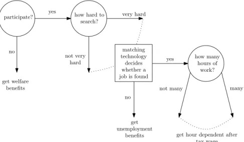
participate? how hard to search?

how many hours of

work?

yes

yes

no

no not very

hard

very hard

many not many

get hour dependent after tax wage get

unemployment benefits get welfare

benefits

matching technology

decides whether a job is found

Figure 1: Sequence of households decisions related to the labor market

happens some time during stage a^R = 5. Stages a∈ {6,7,8} are full retirement stages but with different probabilities of dying 1−γ^a, to better replicate the empirical age structure of the population. As in Blanchard (1985), a reverse life insurance allocates assets at death⁹.

Labor market: After education, households can enter the labor market. They choose whether to participate or not (at a rate δ^a,i ∈ [0,1], which represents the number of time periods of the life-cycle stage with participation). The labor market is imperfect, leading to unemployment. Households who join the labor market start unemployed.

Further, households who have a job may be hit by idiosyncratic unemployment shocks with probability 1−ε^a,i in each time period. Depending on search efforts, a job may or may not be found. If unemployed, households choose job search efforts (s^a,i ≥ 0).

If they have a job, they decide how many hours to work (l^a,i ≥ 0). Being spared the unemployment shock leads to rents, which are bargained with firms to define the wage, building on the static search and matching setting of Boone and Bovenberg (2002).

As in Jaag, Keuschnigg, and Keuschnigg (2010), non-participation in life-cycle a^R is interpreted as retirement. The sequence of households decisions related to the labor market is summarized in figure 1.

Conditional on labor market participation and employment, gross labor income equals

y_lab^a,i =l^a,i·θ^a,i·wⁱ,

whereθ^a,iis an exogenous age-productivity profile calibrated with micro-data and wⁱ is the bargained wage per efficiency unit, assuming separate labor markets for each skill class.

9We use an implementation where the average durations of stay in each life-cycle stage correspond to ages 15-19, 20-24, 25-39, 40-54, 55-69, 70-79, 80-84 and 85+. We later use the words “life-cycle stage”

and “age group” interchangeably.

Household maximization: Households make labor decisions δ^a,i, s^a,i, l^a,i

and con- sumption decisionsC^a,i to maximize their expected life-time utilityV_t^0,i, where V_t^a,i is the expected remaining life-time utility of a household in life-cycle stage a with skill leveli at timet. Preferences are expressed in recursive fashion and restrict households to being risk neutral with respect to variations in income but allow for an arbitrary intertemporal elasticity of substitution:

V_t^a,i= maxh Q^a,i_t ρ

+γ^aβ

GV_t+1^a,iρi1/ρ

,

where ρ defines the elasticity of intertemporal substitution 1/(1−ρ), β is a time dis- counting factor, Q^a,i_t is effort-adjusted consumption, G = 1 +g is the gross factor of growth by which the model is detrended.

Labor market activity generates disutility. Effort-adjusted consumption Q^a,i cap- tures the utility cost of labor market activity expressed in goods equivalent terms, with

Q^a,i = C^a,i−ϕ¯^a,i δ^a,i, s^a,i, l^a,i ,

and ϕ¯^a,i a convex increasing function in all its arguments. Specifically,

¯

ϕ^a,i = δ^a,i

1−u^a,i

ϕ^L,i l^a,i

+ 1−ε^a,i

ϕ^S,i s^a,i + ϕ^P,i δ^a,i

− 1−δ^a,i+δ^a,iu^a,i h^a,i,

where u^a,i ∈[0,1]represents the fraction of time in unemployment, h^a,i is the value of home production if the household is not working,ϕ^L,i captures the disutility of working, ϕ^P,i the disutility of participation and ϕ^S,ithe disutility of job search efforts.

Given the Blanchard (1985) insurance, the budget constraint of households is:

Gγ^a,iA^a,i_t+1=Rt+1

A^a,i_t +y^a,i_t −C_t^a,i

,

whereA^a,i represent assets,y^a,inet income flows andR = 1 +r the gross interest rate.

Social security: Before retirement, non-participants receive (net) welfare benefits y_nonpar^a while unemployed workers receive (gross) unemployment benefitsb^a,i=bⁱ·y_lab^a,i, where bⁱ is the skill-dependent replacement rate. After retirement, households re- ceive (net) pension benefits y^a,ipens = ν^aP^a,i +P₀^a, where P₀^a is a flat part, P^a,i rep- resents acquired pension rights andν^ais a conversion factor between pension rights and pension payments. Pension rights accumulate with labor earnings, following P_t+1^a,i = δ_t^a,i

1−u^a,i_t

y_lab,t^a,i +P_t^a,i.

Taking labor income taxes and social security contributions τ_t^a,i into account and assuming that each labor market state (i.e. non-participation, unemployment and em-

ployment) is visited in each time period¹⁰, net household income amounts to:

y^a,i=











1−τ^a,i δ^a,ih

1−u^a,i

y_lab^a,i+u^a,ib^a,ii

+ 1−δ^a,i

y_nonpar^a if a < a^R, 1−τ^a,i

δ^a,i h

1−u^a,i

y_lab^a,i+u^a,ib^a,i i

+ 1−δ^a,i

ypens^a,i if a=a^R,

ypens^a,i if a > a^R.

Production: Production is made by a competitive representative firm taking input prices as given, namely wage rates, the interest rate and the price of the output good, which serves as numeraire. Changes in the production process are costly variations in the capital stock, and are subject to convex capital adjustment costs, following Hayashi (1982).

The production function is linear homogenous:

Y_t=F^Y

K_t, L^D,i=1_t , L^D,i=2_t , L^D,i=3_t .

The labor inputs L^D,i_t from different skill classes are not perfect substitutes. Con- sistent with empirical evidence (Griliches, 1969), we assume that high skill labor and capital are more complementary than low skill labor and capital and use a nested CES- specification F^Y from Jaag (2009).

Firms make investmentI_tand hiring decisions to maximize the flow of dividends they can generate. Formally, the firm maximizes its end of period value W, which equals the stream of discounted dividend paymentsχ:

Wt=W (Kt) = max

It,L^D,i_t

χt+GW(Kt+1) R_t+1

, s.t. χt=Yt−It−J(It, Kt)−X

i

(1 +τ^F,a)wⁱ_tL^D,i_t , GK_t+1= 1−δ^K

K_t+I_t,

whereJ(·) denotes the adjustment costs andτ^F,a the firms social security contribution rate. Labor demands are pinned down by the marginal products and the labor costs, which consist of wage and contribution rates, i.e. Y_LD,i = (1+τ^F,a)wⁱ. Given an interest rate, investment is defined so that the return on financial investments (the interest rate) equals the marginal cost of investment (Tobin’s q), which depends on the marginal product of capital, net of capital adjustment costs and depreciation¹¹.

Government: Government provides welfare benefits, unemployment insurance, pay- as-you-go pensions and investment subsidies. State expenditures also include public consumption, long-term care and health expenditures, all defined exogenously in per capita terms and generating no utility.

10The assumption follows Jaag, Keuschnigg, and Keuschnigg (2010).

11In steady-state, the capital stock is stable so that there are no capital adjustment costs. In this case, investment satisfies the standard condition where the interest rate equals the marginal product of capital net of depreciation,r=F_K^Y −δ^K.

To finance expenditures, the government collects consumption taxes, labor and cap- ital income taxes, profit taxes, firm and worker social security contributions. The gov- ernment can borrow on the capital market (with or without premium on the interest rate) to finance public debt, to meet some exogenously defined target (most of the time kept constant in simulations).

Single-country equilibrium: In a single-country setting, we assume that the gross interest rateRt+1 = 1+rt+1is exogenously defined, as for small open economies. Savings can be invested in firms, government debt and foreign assets. Assuming no arbitrage, the net returns on these three types of assets are the same and equal to the interest rate rt+1.The goods market then clears because of trade with the rest of the world:

Y_t=C_t+I_t+G_t+T B_t,

where C_t is the aggregate private consumption¹², G_t is government expenditure and T Bt is the trade balance. Holding of foreign assets by domestic households evolves with changes in the trade balance:

D^F_t+1=Rt+1 D^F_t +T Bt

.

Private household assets At are invested in the domestic representative firm Wt, government debtD^G_t and foreign assetsD^F_t , so that the asset market clearing condition is satisfied:

At=Wt+D_t^G+D^F_t . 2.2 Extension to a multi-country setting

We follow Boersch-Supan, Ludwig, and Winter (2006), an extension of the two-country Buiter (1981) procedure to any number of countries and capital adjustment costs. We assume that labor is immobile, that capital is perfectly mobile and that all countries belong to a currency union and produce the same composite good. The interest rate is no longer exogenous, but endogenous.

Equilibrium: Under these assumptions, the equilibrium interest rate must be the same in all countries. The intuition is as follows. Assume there is an arbitrage opportu- nity. Investors in the low interest rate country start to invest in the high interest rate country. The capital stock in the first country declines, increasing the marginal product of capital and thus the interest rate in that country. The opposite happens in the second country. This continues until an equilibrium is reached where the two interest rates are identical.

As a whole, the set of countries is a closed economy, where the interest rate adjusts so that the goods market clear. The resulting equilibrium interest rate is thus the unique

12So, Ct=P

i

P

aN_t^a,iC_t^a,i whereN_t^a,i is the number of households alive at timet, member of age groupaand skill groupi. Other households-related aggregate variables are defined in a similar fashion, including aggregate financial assetsAt.

value such that the goods market clear over all countries. Formally, considerM countries indexed byj∈ {1, ..., M}. Assume that terms of change are fixed and that each variables are normalized so that the numeraire value, after currency-exchange corrections, is the same in all countries. The interest rate is then the unique value such that

X

j∈{1,...,M}

T Bj,t = 0.

Rest of the world: We do not consider all countries in the world but restrict policy analysis to a smaller subset¹³, too small to be isolated from the world capital markets.

Consistent with empirical evidence, the goods market, as a whole, will not clear over this subset. We thus consider a large synthetic Rest-of-the-world country (or a small group of Rest-of-the-world countries), which will account for trade with the rest of the world.

The goods market will clear over all countries which are either part of the subset, or one of the Rest-of-the-world countries. Compared to a case without a Rest-of-the-world country, the adjustment of the equilibrium interest rate is dampened. This reflects access of all countries to the world capital market.

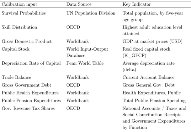
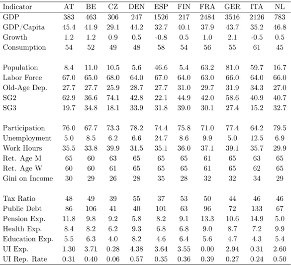
2.3 Calibration

The basis for the multi-country model is a single country model calibrated for 14 Euro- pean countries used for policy evaluation. The calibration of the multi-country model is thus inherited from the single country models, with the exception of the Rest-of-the- world country. We first summarize the calibration part which is inherited and then provide details for the calibration of the Rest-of-the-world country.

Where available, we take consensual empirical estimates from the literature. The equilibrium interest rate is 5%. In crisis time and over the long run, we assume that public debt is a safe asset issued in nominal terms, which are not growing either with inflation nor productivity growth, resulting in a 4 percentage points discount on the price of public debt. Production function specifications are adopted from Jaag (2009).

Labor supply elasticities are derived from Immervoll, Kleven, Kreiner, and Saez (2007) and productivity profiles from Mincer wage regressions on EU-SILC microdata. Average participation rates, unemployment rates and working hours per age and skill classes are computed from LFS and EU-SILC datasets. Parameters for institutions are derived using the European Commission MISSOC database and OECD’s Tax-Benefit model.

Intervivo transfer parameters are calculated to generate life-cycle consumption profiles in line with empirical evidence.

To be able to reflect large economic differences between countries to some extent without including many single countries, we model and calibrate a North rest-of-the-

13In the implementation, the subset contains 14 countries member of the European Union, namely Austria, Belgium, Czech Republic*, Denmark, Finland, France, Germany, Italy, The Netherlands, Poland*, Slovakia, Spain, Sweden* and the UK*. In this list, stars identify the four countries whose currency is neither the Euro nor pegged to the Euro, and thus do not meet our assumption of fixed exchange rates. We keep these countries in the list to have broader diversity. In reality, exchange rate variations absorb some of the country-specific shocks, reducing the size of cross-country spillovers for these four countries, ceteris paribus. Our quantitative analysis illustrates for these countries some consequences of joining the Eurozone.

world country (NROW) and a South rest-of-the-world country (SROW). While we do not model impacts outside the EU, we capture the impact of forces coming from outside of the EU, in line with our objective. We choose to aggregate Canada, Japan and the USA to form the stylized NROW country while we choose Brazil, China and India to form the SROW country¹⁴.

The calibration process rests on macro- and micro-level data, either as direct inputs or as calibration targets. Macro-level data is in general available for all six countries forming the NROW and SROW, in data sources which include the ILO, the OECD, the UNESCO and the World Bank.

Micro-level data on the other hand is not available for all of the six countries. For the sake of consistency, we ignore micro-level data specific to Rest-of-the-world countries.

We follow instead a three step approach. First, for each of the six Rest-of-the-world country, we identify a twin country (or a set of countries) from our sample of 14 cali- brated countries whose demographic, economic and policy characteristics are the closest.

Second, we use the micro-level data inputs for this twin country in the calibration pro- cess of the NROW and SROW. Third, we make stylized corrections to the resulting calibration outcome where there are documented differences.

This approach results in using micro-level calibration inputs from the UK for Canada, Japan and the USA and an average of calibration inputs from the Czech Republic, Slo- vakia and Poland for Brazil, China and India. The most important stylized corrections are proportional adjustments to the participation and unemployment rates by age and skill classes to match the aggregate participation and unemployment rates¹⁵.

3 Quantitative analysis

In this section we perform simulations with the multi-country overlapping-generations model to analyze cross-country fiscal policy spillovers when production exhibits capital- skill complementarity. When one large country performs a reform, we quantify out- put spillovers on the remaining thirteen countries included in our scope. We find that spillovers differ by country and investigate sources for the differences. A summary of findings ends the section.

3.1 Cross-country fiscal policy spillovers

We perform two realistic policy reforms in Germany, the largest country in our sample, and quantify spillovers on other countries, taking output variations as our core measure of aggregate economic activity. The first reform consists of a 20% labor income tax cut financed by an increase in consumption taxes (a so-called fiscal devaluation), keeping public debt constant. The extent of the tax cut corresponds to standard policy reforms in normal times.

By contrast, we consider in the second reform drastic measures which are only applied in crisis times. As Corsetti, Meier, and Müller (2012) have shown empirically, domestic

14With these choices we are capturing close to 60% of the actual real world GDP and five of the eleven most important trade partners of the EU, together reflecting more than 40% of total trade of the EU.

15Further details on the calibration of the Rest-of-the-world countries are contained in appendix A.

fiscal multipliers are larger during financial crises. We thus conjecture larger cross- country spillover effects during crises. According to the International Monetary Fund (2013), the public support provided by German authorities to its financial sector after the 2007 subprime crisis amounted to 10.8% of GDP. Taking into account that other sectors may have benefited from public support too, we consider public expenditures increases of 2.5% of GDP during 5 years to support recovery efforts of private agents in a pure balance sheet fashion. The crisis is financial, without any damage to production capacity. We investigate the long-term consequences of the private sector bailout after the crisis is finished. Whether of own decision or because of external pressure, we assume in this subsection that German authorities keep their public debt constant at all times, thanks to an increase in labor income taxes. Another treatment of public debt will be analyzed in subsection 4.1.

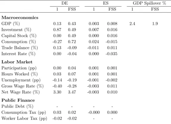
There are no fiscal policy reforms in other countries, except a passive adjustment of consumption taxes (first reform) or labor income taxes (second reform) to keep public debt constant. Table 1 provides a selection of results for the first reform while table 2 provides a selection for the second reform¹⁶. We discuss each reform in turn.

DE ES GDP Spillover %

1 FSS 1 FSS 1 FSS

Macroeconomics

GDP (%) 0.13 0.43 0.003 0.008 2.4 1.9

Investment (%) 0.87 0.49 0.007 0.016 Capital Stock (%) 0.00 0.49 0.000 0.016 Consumption (%) -0.27 0.72 0.024 -0.015 Trade Balance (%) 0.13 -0.09 -0.011 0.011 Interest Rate (%) 0.00 -0.04 0.000 -0.035 Labor Market

Participation (pp) 0.00 0.04 0.001 0.001 Hours Worked (%) 0.03 0.07 0.001 0.001 Unemployment (pp) -0.14 -0.19 -0.001 -0.002 Gross Wage Rate (%) -0.40 -0.28 -0.003 0.011 Net Wage Rate (%) 3.30 3.47 -0.003 0.010 Public Finance

Public Debt (%) - - - -

Consumption Tax (pp) 0.03 0.02 -0.000 0.000 Worker Labor Tax (pp) -0.02 -0.02 - -

Legend: 1 = year of impact,FSS = Final Steady State,(%)= changes in percentage from initial steady state,(pp) = changes in percentage points from initial steady state,Tax = average tax rates over all age and skill groups,GDP Spillover %= percentage change in GDP (%) in ES compared to change in GDP (%) in DE.

Table 1: Labor tax cut in Germany financed by consumption taxes

Outcomes of first reform (moderate labor tax cut)

Table 1 displays macroeconomic, labor market and public finance impacts for the reform

16Appendix B provides spillover effects for all reforms considered in this paper for all countries.

country, Germany, and the country where spillovers are largest, Spain. The table shows that the output spillovers are small, on impact (GDP increases in Spain 2.4% of the increase in Germany) and over the long run (1.9%) when Germany reduces labor income taxes by 20% and finance it with an increase in consumption taxes.

The reason for the spillovers is the integrated capital market. On impact, the tax cut in Germany stimulates domestic labor supply (e.g. -0.14 percentage points unemploy- ment) and increases production (+0.13%). However, the increase in the consumption tax reduce consumption not only from active households, but also retired households.

Aggregate consumption thus drops (-0.27%), which, combined with higher production, increases the demand for savings on the international capital market, materialized by an increase in the trade balance (+0.13%). Spain invests and consumes part of the ad- ditional capital market liquidity, which increases the consumption tax base and allows the Spanish government to reduce its consumption tax rate while keeping its public debt constant, which stimulates local labor supply and production (+0.003% on impact).

The magnitude of the spillover remains small, however (2.4% on impact and 1.9%

over the long run). There are two contributing factors. First, the reform is of relatively small magnitude, so that German investors are able to absorb domestically a large part of the savings shock (investment increases 0.87%). Second, the liquidity increase in the international capital market benefits not only Spain, but the other 13 countries and the rest of the world as well.

DE ES PL

7 Avg 7 Avg Spill % 7 Avg Spill %

Macroeconomics

GDP (%) -0.45 -0.59 -0.20 -0.14 24.4 -0.09 -0.06 10.0

Investment (%) 0.03 -0.20 -0.05

Capital Stock (%) -0.52 -0.33 -0.20

Consumption (%) -1.69 -0.10 -0.03

Trade Balance (%) 0.67 -0.11 -0.06

Interest Rate (%) 0.43 0.43 0.43

Labor Market

Participation (pp) -0.06 -0.03 -0.02

Hours Worked (%) -0.07 -0.03 -0.01

Unemployment (pp) 0.09 0.05 0.02

Gross Wage Rate (%) -0.07 -0.16 -0.10

Net Wage Rate (%) -0.86 -0.34 -0.16

Public Finance

Public Debt (%) - - -

Consumption Tax (pp) - - -

Worker Labor Tax (pp) 0.52 0.13 0.05

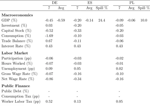
Legend: 7 = 7 years after reform start,Avg = yearly average changes over the medium run (years 1 to 25) in percentage,Spill % = average GDP spillover in percentage, equal to yearly average change of GDP in ES (resp. PL) over yearly average change of GDP in DE. See table 1 for more.

Table 2: Large and temporary public spending increase in Germany with constant public debt

Outcomes of second reform (large temporary government spending increase) Table 2 provides economic impacts of a large but temporary government spending in- crease in Germany, where public debt is kept constant with increases in labor income taxes. Simulated impacts are provided for Germany (the reform country), Poland (where spillovers are smallest) and Spain (where spillovers are largest). Detailed outcomes two years after the end of the spending increase (in period 7) are provided, as well as the average output variation over the medium run (in columnAvg), arbitrarily defined as a 25 years time horizon¹⁷.

The table shows that output spillovers can be sizable, as the average output loss in Spain (-0.14% per year) is almost a quarter of the average output loss in Germany (-0.45%). The table also shows that the spillover varies across countries: while it is almost 25% in Spain, it is only 10% in Poland. In the continuation we discuss the first finding. The second finding will be investigated in subsection 3.2.

Integrated capital markets and capital-skill complementarity explain why spillovers can be large. The intuition is as follows. The large public spending increase in Germany (+2.5% of GDP during 5 years) is a drag on the capital market which crowds out private investment in all countries (from -0.52% in Germany to -0.20% in Poland after seven years), thus reducing the capital stock and output in all countries.

Capital-skill complementarity deepens output spillovers. Indeed, capital-skill com- plementarity means that capital is more complementary to high-skilled labor in pro- duction than to low-skilled labor. If capital is an important complement to the most productive types of labor, the negative impact of capital scarcity on output is magni- fied. This applies to the reform country (Germany) and any country integrated in the same capital market (Poland and Spain). If there was no capital-skill complementarity in production, the negative impact on output would be smaller, since capital would be equally complementary across all types of labor.

Another factor, standard, contributes to the negative impact on output, namely distortive taxation. To keep public debt constant with a decrease in capital and thus wage rates, the labor income tax rate needs to be increased, which depresses labor supply and further drags output down. Note however that this factor was also operating in the case of the first reform (20% cut in labor income taxes in Germany, financed by larger consumption taxes). Alone however, this factor did not lead to large spillovers: the domestic increase in savings was sufficient to absorb most of the additional demand on the integrated capital market (as shown for instance by the smaller interest rate variation in table 1 than in table 2).

3.2 Cross-country differences in spillovers

Table 2 shows that the average yearly output loss over the medium run is 0.14% in Spain and 0.06% in Poland when Germany makes a large but temporary increase in government spending, Germany itself losing an average yearly 0.59% of output. We

17If we were to discount future output variations, we would implicitly use a social welfare function which puts higher weight on current generations and lower weight on future generations. We choose to remain neutral and apply no discounting.

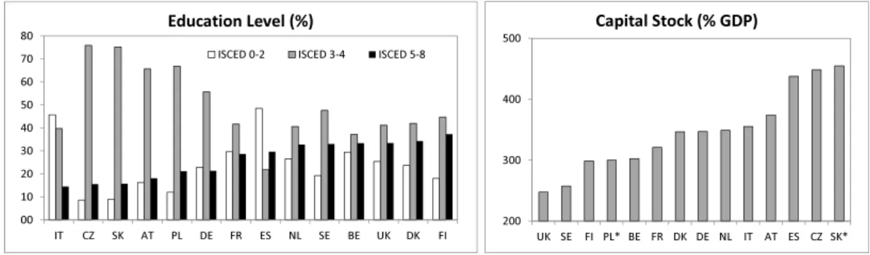
Sources: OECD Education at a Glance; OECD Structural Analysis (STAN) database (average 2001-2007); *:estimate 00

10 20 30 40 50 60 70 80

IT CZ SK AT PL DE FR ES NL SE BE UK DK FI

Education Level (%)

ISCED 0-2 ISCED 3-4 ISCED 5-8

200 300 400 500

UK SE FI PL* BE FR DK DE NL IT AT ES CZ SK*

Capital Stock (% GDP)

Figure 2: Initial education and capital stock characteristics

investigate the reasons for differences in the size of spillover across countries and show that production inputs and production structure play a key role, including capital-skill complementarity.

Figure 2 provides a view of key production inputs for the 14 countries in our scope.

One can observe that Poland and Spain lie at opposite extremes: Poland has one of the smallest capital stock (as fraction of GDP) and one of the smallest amount of skilled households (educated at ISCED 5-8 levels), while Spain has one of the largest amount of capital stock and skilled households.

In the initial equilibrium, the outcome of calibration is a larger weight on capital and skilled labor inputs into production, leading to a larger degree of capital-skill comple- mentarity, in Spain. Recall indeed that production parameters, which define the degree of capital-skill complementarity, are calibrated to match output, the marginal product of capital and other production targets, taking production inputs from the data. All of these parameters and values are country-specific. However, in an integrated capital market the interest rate and thus the marginal product of capital are identical across countries. The production weights on skilled labor and capital are therefore largest in countries where the supply of these production factors are largest¹⁸.

As discussed at the end of subsection 3.1, capital-skill complementarity tends to amplify the magnitude of spillovers: the public spending increase in Germany draws resources from the integrated capital market, reducing investment and thus capital and output in all countries, an effect which is magnified when capital is complementary to skilled labor in production. The degree of capital-skill complementarity being larger in Spain, and smaller in Poland, the spending increase in Germany has largest effects in Spain and smallest in Poland.

To further investigate the contribution of production inputs and production structure in spillovers, we perform a quantitative decomposition analysis. We consider counter- factual calibration scenarios in Spain and Poland, leaving calibration of other countries

18Semi-formally, consider the simpler case of Cobb-Douglas productionYj =K_j^αj(AL)^1−αj for dif- ferent countries j ∈ {1,2, ..., M} with identical labor inputs and labor-augmenting technologies, but different capital supplies Kj and capital contributions αj. An identical marginal product of capital αj(AL/Kj)^1−αj means that the largest capital contribution αj comes for the country with largest capitalKj.

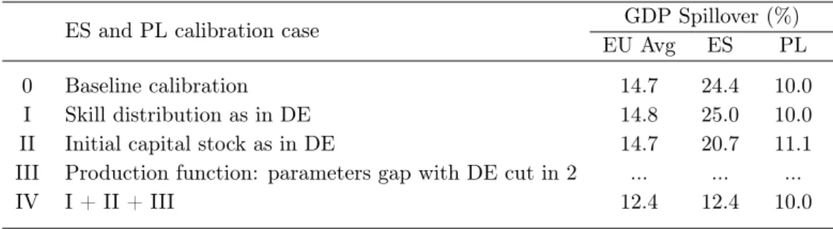
unchanged. The same government spending reforms in Germany as in subsection 3.1 is then applied and leads to spillovers which are compared with the baseline case.

ES and PL calibration case GDP Spillover (%)

EU Avg ES PL

0 Baseline calibration 14.7 24.4 10.0

I Skill distribution as in DE 14.8 25.0 10.0

II Initial capital stock as in DE 14.7 20.7 11.1

III Production function: parameters gap with DE cut in 2 ... ... ...

IV I + II + III 12.4 12.4 10.0

Legend: GDP Spillover (%) = yearly average change of GDP in ES (resp. EU Avg, PL) over yearly average change of GDP in DE over the medium run (years 1 to 25),EU Avg = average for all 14 EU countries except DE. Calibration of other countries than ES and PL remains unchanged. The reform is the same as in table 2, a large public spending increase in Germany with constant public debt.

Table 3: Large and temporary public spending increase in Germany: decomposition analysis Table 3 provides an overview of the decomposition and the results. Several produc- tion calibration scenarios are considered and illustrate the role of the various production components in spillovers size.

Case0 represents the baseline calibration scenario, where production parameters are outcomes of actual empirical observations. As in table 2, the output spillovers are 24.4%

for Spain and 10.0% for Poland. The average spillover size over all countries (except Germany) is 14.7%.

Case I assumes that the skill distribution in Spain and Poland is the same as in Germany, according to the graph in the left of figure 2. The skill distribution of other countries remains unchanged. When Germany then performs the same government spending reform as in the baseline scenario, the spillover in Spain increases to 25.0%

and the average spillover to 14.8%, while it remains constant in Poland. Differences in skilled labor inputs in production thus do not represent the main reason for differences in spillover sizes.

CaseII assumes that the capital stock in the initial equilibrium is the same in Spain and Poland as in Germany (as % of GDP). After the spending reform in Germany, the spillover in Spain decreases to 20.7% while the spillover in Poland increases to 11.1%.

Part of the differences in spillover sizes are thus due to differences in capital input into production.

Case III changes the production function parameters in Spain and Poland. Specifi- cally, the difference between the parameters in Spain (respectively Poland) and Germany is reduced by 50%. This counterfactual change in production structure without change in production inputs leads to unusual economic equilibrium, generating difficulties in numerical solutions.

Case IV combines the changes in calibration in Spain and Poland that are applied in casesI,II andIII: the skill distribution and initial capital stock have the same values as in Germany and the gap in production function parameters with German values is cut in two. After the government spending increase in Germany, spillovers in Spain,

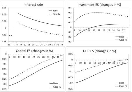
-0.35 -0.3 -0.25 -0.2 -0.15 -0.1 -0.05 0

7 10 13 16 19 22 25 28 31 34 37

Capital ES (changes in %)

Base Case IV

-0.25 -0.2 -0.15 -0.1 -0.05 0 0.05

7 10 13 16 19 22 25 28 31 34 37

GDP ES (changes in %)

Base Case IV -0.3

-0.2 -0.1 0 0.1 0.2 0.3 0.4

7 10 13 16 19 22 25 28 31 34 37

Investment ES (changes in %)

Base Case IV 4.98

4.99 5 5.01 5.02 5.03

ISS . . . 6 9 12 15 18 21 24 27 30 33 36 39

Interest rate

Base Case IV

Figure 3: Outcomes for Spain after spending increase in Germany, different calibrations Poland and other countries change: the output spillover in Spain now equals the average spillover among all countries (at 12.4%) while the gap between the spillover in Poland and all other countries is reduced, compared to the baseline (2.4 instead of 4.7 percentage points).

The intuition is the following. Changes in production inputs and structure leads to a lower capital-skill complementarity and lower demand for capital in Spain. The resulting equilibrium interest rate, before and after the reform in Germany, is lower.

Investments are cheaper. Because the degree of capital-skill complementarity is reduced in Spain, its magnifying effect on spillover is lower (as discussed at the end of subsection 3.1). Figure 3 illustrates the difference in interest rates, investments, capital stocks and outputs between the baseline case and caseIV after the reform. In particular, the figure shows that the output loss is smaller in caseIV (dotted line) than in the baseline (plain line).

Two conclusions emerge from the decomposition analysis. First, differences in pro- duction inputs and structure, including capital-skill complementarity differences, play an important role in the difference in the size of fiscal policy spillovers. With identical production inputs and 50% less differences in the production structure as in Germany, output spillovers in Spain are no longer greater than in other countries, but equal to the average spillover value. Second, these disparities in production inputs and structure are not the only factors which leads to spillover size differences. The same counterfac- tual transformation of production inputs and structure in Poland as in Spain leads to spillovers in Poland which are closer, but not equal to spillovers in other countries: they remain smaller than average¹⁹.

19This second conclusion also motivates the partial, rather than full, removal of production structure differences with Germany in casesIII andIV: the gap in production parameters is not removed 100%, but only 50%.

3.3 Summary of findings

This subsection consolidates findings from the quantitative analysis and then summarizes key mechanisms at work.

Finding 1. The cross-country spillovers of a standard labor income tax are small: when Germany cuts its labor income tax rate 20% and increases its consumption taxes to keep public debt constant, the largest output gain in other countries amounts to 2.5% of the output gain in Germany.

Finding 2. The cross-country spillovers of a large and temporary government spending increase can be sizable: when Germany increases its public spending 2.5% of GDP during 5 years and keeps its public debt constant with higher labor income taxes, the largest average yearly output loss over the next 25 years in other countries amounts to 24.4%

of the average yearly loss in Germany.

Finding 3. The size of cross-country spillovers varies across countries: the German reform in Finding 2 leads to output losses in other countries which range from 10.0% to 24.4% of the output loss in Germany.

Spillovers in the first finding are due to the integration of the capital market. The labor tax cut and consumption tax hike stimulates labor supply and output in Germany, but drops aggregate consumption. On impact, Germany increases savings and fuels the capital market. Other countries can invest more.

Together with the integrated capital market, capital-skill complementarity explains the second and third findings. The large public spending hike in Germany crowds out private investment in all countries. The capital stock drops, reducing output. The output drop is magnified by capital-skill complementarity, as the contribution of the most productive type of labor to production is reduced with the capital drop. Countries where production exhibits a large degree of capital-skill complementarity suffer more than others.

4 Policy implications

We use the model to investigate the effect of debt management rules, which may be defined at the country level or come from a fiscal policy coordination framework. We then derive policy implications for fiscal policy coordination.

4.1 Alternative public debt management rules

Section 3 showed that cross-country fiscal policy spillovers can be small or large, for realistic reform scenarios. All cases that were considered assumed that public debt was to remain constant at all times, for internal or external policy reasons. In this section we consider alternative public debt management rules for the reform which generate

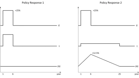
Policy Response 1 Policy Response 2

year year

+12.5%

DG DG

1 6 1 6 25

G G

τ τ

+25% +25%

Legend: G= public spending,τ= labor income tax,DG= public debt

Figure 4: Public spending increase: stylized representation of alternative fiscal policy responses

-2.0%

-1.5%

-1.0%

-0.5%

0.0%

1 7 13 19 25 31 37 43 49

GDP (changes in %) DE

Response 1 Response 2

Figure 5: Germany output following public spending increase, alternative debt treatments the larger spillovers, a large a temporary increase in government spending in Germany (+2.5% of GDP over five years) with labor income tax variations to match public debt targets.

In the previous section, the target was a constant public debt. Here, we assume that public debt may temporarily increase, up to 12.5% of its current value, but that it has to be back to its original level after 25 years. While the first policy response leads to a large but short-lived increase of labor income taxes, the second response leads to a mild but prolonged increase of the taxes. Figure 4 illustrates the difference between the two policy responses.

Results of the simulations, which compare the impact of the two policy responses over time, are presented in figure 5 and table 4.

The figure provides the output path in Germany over the long-run. It shows that the output loss is larger when debt is not allowed to increase (policy response 1; dotted line) than when the debt can increase (policy response 2; plain line) but that peak in the loss lasts fewer years. This result is not surprising, as the output loss mimics the variation in labor income taxes (recall figure 4). The figure however does not allow to see which of the two policy responses is the most damaging for output on average. The

answer appears in table 4.

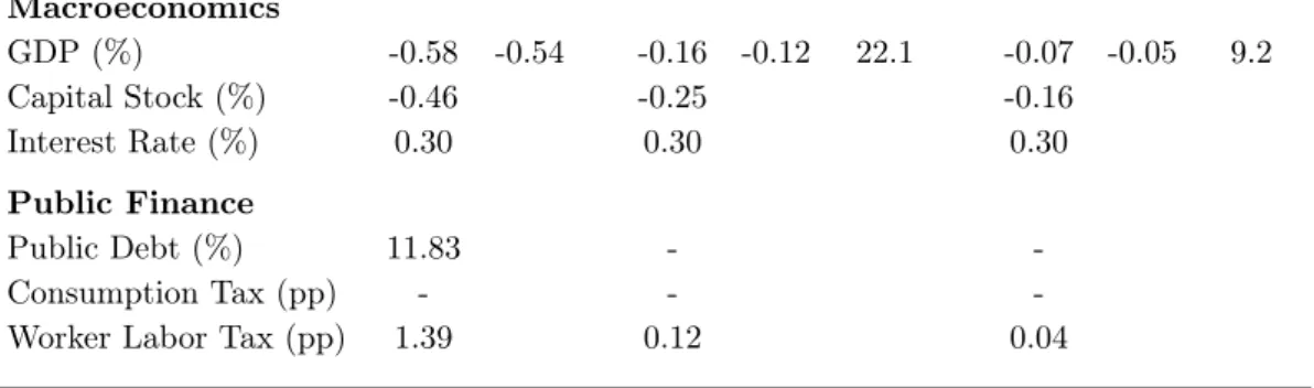
DE ES PL

7 Avg 7 Avg Spill % 7 Avg Spill %

Panel A. Policy Response 1: no increase in public debt

Macroeconomics

GDP (%) -0.45 -0.59 -0.20 -0.14 24.4 -0.09 -0.06 10.0

Capital Stock (%) -0.52 -0.33 -0.20

Interest Rate (%) 0.43 0.43 0.43

Public Finance

Public Debt (%) - - -

Consumption Tax (pp) - - -

Worker Labor Tax (pp) 0.52 0.13 0.05

Panel B. Policy Response 2: temporary increase in public debt

Macroeconomics

GDP (%) -0.58 -0.54 -0.16 -0.12 22.1 -0.07 -0.05 9.2

Capital Stock (%) -0.46 -0.25 -0.16

Interest Rate (%) 0.30 0.30 0.30

Public Finance

Public Debt (%) 11.83 - -

Consumption Tax (pp) - - -

Worker Labor Tax (pp) 1.39 0.12 0.04

Legend: see table 2.

Table 4: Large and temporary public spending increase in Germany, alternative debt treatments The table provides selected macroeconomic and public finance outcomes in Germany, Spain and Poland for the two reforms. Panel A displays the impact of the first policy response, where public debt is kept constant. The information is the same as in table 2 and repeated for convenience. Panel B provides the impact of the second policy response, where public debt is temporarily allowed to increase²⁰.

The table shows that the average yearly output loss in Germany is larger when public debt is kept constant (-0.59% versus -0.54%). There are two reasons for such a result.

First, the disruptive effect of taxation increases in an over-proportional manner with the level of taxes, as disutility of labor increases in a convex fashion; although labor income taxes are increased for a shorter amount of time when public debt is kept constant, the increase leads to an over-proportional damage. Second, the spending shock is smoothed across countries with the fiscal policy that keeps debt constant, while it is smoothed across countries and across time with the policy that allows debt to grow temporarily.

The combination of international and intertemporal smoothing is more efficient.

Table 4 also shows that the negative output impacts outside Germany are larger with a constant German public debt than with a temporary debt increase (Spain: -0.14% vs -0.12%; Poland: -10.0% versus -9.2%). In relative terms, the benefits of a larger public

20Appendix C provides for Panel B the information which table 2 provides for Panel A.

debt are even larger in the foreign countries than in the reform country (Germany: 8.1%

gain; Spain: 16.7% gain; Poland: 15.2% gain).

Moreover, the negative spillovers are larger with a constant debt, both in Spain (24.4% vs 22.1%) and in Poland (10.0% vs 9.2%). Because output drops more with a constant debt policy, the need for Germany to draw on foreign resources to finance the public spending hike is larger, increasing the drag on the international capital market (as can be seen in the interest rate, increasing 0.43% vs 0.30% in period 7), which crowds out private investments in all countries to a larger extent.

4.2 Implications for public debt coordination rules

The European Union expects its members to meet a number of fiscal policy targets. In particular, public debt should not exceed 60% of GDP. Drawing from our quantitative analysis, we discuss this fiscal policy coordination target. We argue that there can be benefits for each members of the EU if this debt ceiling rule was relaxed in some circumstances and under certain conditions, even if only one member is facing economic challenges.

The previous subsection showed that the disruptive effects of a large and temporary public spending increase are smaller if public debt is temporarily allowed to increase.

The public spending increase that was considered is large (2.5% of GDP during 5 years) but, in exceptional circumstances, realistic: public transfers to the financial sector fol- lowing the 2007 subprime crisis amounted to 10.8% of GDP in Germany (International Monetary Fund, 2013).

Several factors can explain the high levels of public debt that can be seen in many developed countries. Unsound economic policy may be one factor. Bad luck is another one. Countries which have repeatedly been hit by adverse shocks and have reached the EU debt ceiling, if hit again by another shock, no longer have the room for a temporary increase of public debt. Yet, the temporary increase in public debt allows to reduce economic distortions, which can ease public debt management. Over time, countries with bad luck may end up in growingly weaker economic positions because of coordination rules themselves, rather than their own economic policy (vicious circle).

The EU fiscal rules may thus benefit from an adjustment, seeking to differentiate choice (unsound public finance management) from chance (external negative shock).

The previous subsection also showed that all countries can benefit from rules which allow a temporary debt increase, not only the country hit by the shock. In fact, the benefits may even be larger for the countries not hit by the shock. In the scenario we considered, the output losses are reduced about twice as much in the shock-free countries as in the country hit by the shock, if that country alone can temporarily increase public debt (Germany, hit by the shock: 8.1% gain; Poland, shock-free country with smallest gains: 15.2% gain).

To sum up, if rules or procedures allow to separate choice from chance, allowing a country hit by an adverse shock to increase its public debt beyond the debt ceiling target in a temporary fashion would not only benefit the country hit by the shock itself, but all other shock-free countries too. Shock-free countries may even benefit more from

these alternative public debt coordination rules. Such a conditional debt-ceiling relaxing rule makes efficiency gains because the overall tax distortion is reduced and because the shock on capital markets is smoothed not only across countries, but also across time.

5 Conclusion

We build a multi-country overlapping-generations model with an integrated capital mar- ket in a currency union and calibrate it to cover 14 countries, together covering above 80% of the population of the European Union. Consistent with empirical evidence, we assume that production exhibits capital-skill complementarity. We show that this feature amplifies cross-country spillovers.

In a realistic but large public spending increase scenario, we find for instance that output losses in shock-free countries can amount to a quarter of the loss in the country hit by the shock. Because an increase in public spending crowds out private investments and capital markets are integrated, reform-free countries also experience a decrease in capital stock and output. Capital-skill complementarity deepens output spillovers, because the reduction in capital decreases the contribution of the most productive type of labor.

Different production structures, and thus degrees of capital-skill complementarity, lead to differences in the size of output spillovers across countries. We find that the smallest spillover is 10% (Poland) and the largest 25% (Spain) for the same reform (in Germany).

It is worth stressing out that the only channel for these large output spillovers is the freedom for investors to invest anywhere. A constraint on monetary policy, such as the Zero Lower Bound, is not needed to generate larger spillovers. Our results however remain compatible with earlier findings from the literature and provide a complementary view, highlighting the importance of capital use in production.

Comparing fiscal rules, we show that temporary increases in public debt can reduce the output losses not only in countries which experience a detrimental increase in public debt, but also in other countries. Under certain circumstances and conditions, the European Union may thus benefit from relaxing its 60%-of-GDP debt ceiling rule.

This paper focused on spillovers, considering only a few fiscal policy coordination alternatives. Gains from alternative fiscal policy coordination have been identified, but remain quantitatively small. A more complete investigation of the potential of fiscal policy coordination is left for future research.

The literature generally finds that cross-country spillovers are small when mone- tary policy operates freely, and larger when the ZLB is binding. Future research could also investigate whether spillovers are even larger when both the ZLB and capital-skill complementarity operate.

References

Alessandria, G. and A. Delacroix(2008): “Trade and the (dis)incentive to reform labor markets: The case of reform in the European Union,” Journal of International Economics, 75, 151–166.

Auerbach, A. and Y. Gorodnichenko(2013): “Output Spillovers from Fiscal Pol- icy,” The American Economic Review: Papers and Proceedings, 103, 141–146.

Auerbach, A. J. and L. J. Kotlikoff (1987): Dynamic Fiscal Policy, Cambridge University Press.

Beetsma, R., M. Giuliodori, and F. Klaassen(2006): “Trade Spill-Overs of Fiscal Policy in the European Union: A Panel Analysis,” Economic Policy, 21, 639+641–687.

Benes, J., M. Kumhof, D. Laxton, D. Muir, and S. Mursula(2013): “The Bene- fits of International Policy Coordination Revisited,” IMF Working Paper, WP/13/262, 1–52.

Berger, J., T. Davoine, P. Schuster, and L. Strohner (2016): “Cross-country differences in the contribution of future migration to old-age financing,” International Tax and Public Finance, 23, 1160–1184.

Blanchard, O., C. J. Erceg, and J. Lindé(2016): “Jump-Starting the Euro Area Recovery: Would a Rise in Core Fiscal Spending Help the Periphery?” in NBER Macroeconomics Annual 2016, Volume 31, National Bureau of Economic Research, Inc, NBER Chapters.

Blanchard, O. J. (1985): “Debt, Deficits, and Finite Horizons,” Journal of Political Economy, 93, 223–47.

Boersch-Supan, A., A. Ludwig, and J. Winter(2006): “Ageing, Pension Reform and Capital Flows: A Multi-Country Simulation Model,” Economica, 73, 625–658.

Boone, J. and L. Bovenberg(2002): “Optimal labour taxation and search,” Journal of Public Economics, 85, 53–97.

Botman, D. P., D. Laxton, D. V. Muir, and A. Romanov(2006): “A New-Open- Economy Macro Model for Fiscal Policy Evaluation,” IMF Working Papers 06/45, International Monetary Fund.

Buiter, W. H. (1981): “Time Preference and International Lending and Borrowing in an Overlapping-Generations Model,” Journal of Political Economy, 89, 769–97.

Clemens, M. A. (2011): “Economics and Emigration: Trillion-Dollar Bills on the Sidewalk?” Journal of Economic Perspectives, 25, 83–106.

Cogan, J. F., J. B. Taylor, V. Wieland, and M. H. Wolters (2013): “Fiscal consolidation strategy,” Journal of Economic Dynamics and Control, 37, 404–421.