Project: Development of an Evaluation Framework for the Introduction of Electromobility

Project:

Development of an Evaluation Framework for the Introduction of Electromobility

Deliverable 1.1: Report on Improvements in the Hybrid General Equilibrium Core Model

Due date of deliverable: 30.01.2014

Authors

Michael Gregor Miess, IHS Stefan Schmelzer, IHS

Julia Janke, IHS

Contents

1 Introduction 1

1.1 Research Question . . . . 1

1.2 Assessing the Economic Costs of Electromobility - Modelling Challenges . . . 2

2 Description of the Existing CGE Model MERCI at the Institute for Advanced Studies 5 2.1 Theoretical Structure of MERCI . . . . 5

2.1.1 An Arrow-Debreu Economy in a Complementarity Format . . . . 7

2.1.2 Integrating Bottom-Up in Top-Down . . . . 10

2.1.3 The Dynamics of the Ramsey Model in an MCP Formulation . . . . . 13

2.2 Model Implementation and Application to Austria . . . . 17

2.2.1 Dataset: A Social Accounting Matrix (SAM) for Austria . . . . 17

2.2.2 Short Description of Model . . . . 22

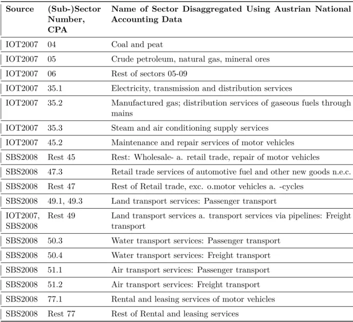
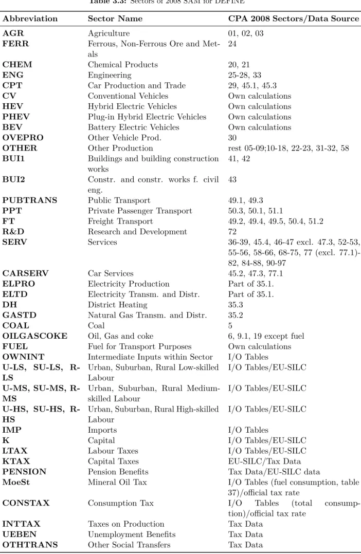
3 Model Extensions in DEFINE 30 3.1 Extentions to Standard Austrian I/O Tables . . . . 30

3.2 Mobility Good - Disaggregation of Transport Sector . . . . 33

3.2.1 CV, HEV, xEVs as separate goods . . . . 33

3.2.2 Household Individual Transport Demand - Modelling Methods . . . . 36

3.2.3 Disaggregation of Engineering Sector and Transport Sector . . . . 39

3.2.4 Construction of Fuel Sector - Electricity Input for xEVs . . . . 40

3.3 Household Disaggregation . . . . 41

3.3.1 Elasticities . . . . 42

3.4 Electricity Sector . . . . 43

3.4.1 Intermediate and Factor Input Structure . . . . 43

3.4.2 Incorporating Results of Detailed Electricity Market Models . . . . 44

3.5 Calibrating the CGE Model . . . . 46

4 Applicability of Improved Model to Modelling Challenges 47 4.1 Modelling of Measures for Electromobility . . . . 47

4.2 Expected Results . . . . 49

5 Outlook 51 5.1 First View on Scenarios . . . . 51

Bibliography 52

List of Figures 56

List of Tables 57

Nomenclature 58

CHAPTER 1

Introduction

1.1 Research Question

The aim of DEFINE

is to estimate and assess the full economic costs that coincide with raising the share of electric mobility in the transport system (for Austria, Germany and Poland), taking account of the electricity system and environmental externalities.

To this end, the macroeconomic system in sectoral disaggregation, the electricity producing system on a technology level, the transport system , household preferences and environmental effects are considered during the course of the analysis by using and developing suitable modelling tools.

For a comprehensive integration of the factors of analysis, the structure of the existing computable general equilibrium (CGE) model at the Instute for Advanced Studies (IHS) MERCI

, which is mainly based on a theoretical model developed by Böhringer and Rutherford (2008, [5]), provides a suitable framework for analysis. Combining a general top-down sectoral macroeconomic view of the economy with an electricity sector incorporating technology detail makes it possible to assess the costs of both increasing the share of electric mobility in the transport system and the corresponding effect on the electricity production system.

However, before a realistic macroeconomic "price tag" can be placed on a medium to large scale introduction of electromobility, especially in the sphere of individual motorized transport, the amount of detail in depicting the transport sector within the macroeconomic model has to be increased and brought closer to reality.

To achieve this, a couple of extensions regarding the transport sector, especially concerning the preferences of households when it comes to car purchase and mode choice, were foreseen for DEFINE. After a detailed introduction into the theoretical background and structure of the IHS CGE model (chapter 2), chapter 3 of this report describes the extensions conducted

1 Development of an Evaluation Framework for the INtroduction of Electromobility 2 Model for ElectRicity and Climate change policy Impacts

in DEFINE, also in regard to the findings of the first theoretical modelling workshop with Prof. Christoph Böhringer (University of Oldenburg) in November 2012.

1.2 Assessing the Economic Costs of Electromobility - Modelling Challenges

The top-down bottom-up structure allows to combine scenarios regarding the introduction and acceptance of electromobility in a general equilibrium framework with information about the provision of electricity on a technology level . Electromobility in this study primarily relates to individual passenger transport , but the mode choice of the household agents between individual and public transportation is also incorporated . To ensure a realistic modelling approach, several challenges have to be met that will be described in the following before displaying the basic structure of the model.

Micro-Data Firstly, since electromobility for individual transport, i.e. electric vehicles (xEVs)

, has not been introduced on a large scale in Austria, Germany or Poland, the present preference structure estimated from empirical studies and implemented within the IHS CGE model might not correctly depict the preferences of the consumers regarding the substitution of conventional vehicles (CVs)

fuelled by gasoline or diesel with electrically powered vehicles of different kinds. To address this shortcoming, a detailed household data survey has been conducted in DEFINE to firmly root the CGE modelling effort in empirical data. Most importantly, the preferences of the Austrian/Polish population regarding the purchase of alternatively-fuelled vehicles and/or transport mode choice have been/will be retrieved in representative surveys in Work Packages (WP) 3 and 8 of the DEFINE project.

The Austrian survey has already been completed and the respective models estimated until fall 2013. From this survey, elasticities of substitution within the consumption function of the representative households were estimated, and information about mobility behaviour of households living in different areas according to popolation density can already be deduced accordingly at the point of writing this report.

Disaggregation of Representative Household To accomodate the structure of the household survey and capture the different natures of distinct household types, the representative household of the IHS CGE model MERCI is disaggregated according to the population density of the main place of residence (urban, sub-urban and rural) and the highest education attained (3 skill groups). The first dimension shall depict different mobility needs and availability of alternative transportation modes to individual transport, such as public transport in various forms. The second dimension of highest education attained shall capture income possibilies of the household as well as a difference in environmental preference. Therefore, the heterogeneity

3 Electric vehicles (xEVs)in this terminology comprise both battery electric vehicles (BEVs) and plug-in hybrid electric vehicles (PHEVs).

4 Or hybrid electric vehicles (HEVs), which will constitute another form of CVs with higher fuel efficiency, since they do not directly use electric power as fuel, but rather generate it from stop-motion in traffic.

1.2 Assessing the Economic Costs of Electromobility - Modelling Challenges

of household preferences depicted in the micro data shall be replicated in the CGE model along its main dimensions. This is a starting point for analysis: one might e.g. expect xEVs to be picked up faster in urban areas due of their, as compared to CVs, low driving range, and among people of university education that have, on average, a higher income, by which they can afford the comparably rather expensive electric vehicles, and maybe also exhibit different environmental preferences. Educated guesses such as the latter should be subjected to careful model- and data-guided analysis.

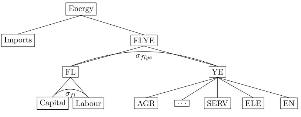
Disaggregation of Macro-Data (SAM) Another factor is the disaggregation of macro data. In order to model the household consumption decision between individual transport and public transport on the one hand, and then between different modes of individual transport, i.e.

CVs, hybrids, xEVs, on the other, these different transport modes/purchase choices have to be separate goods in the Social Accounting Matrix (SAM) serving as a database for the IHS CGE model. Since these goods are not represented separately in the Input-Output (I/O) tables provided by Statistics Austria

, they have to be carefully derived from the I/O tables of statistics Austria under some assumptions and using additional data sources.

Electricity Production Moreover, the additional load of xEVs for the electricity system will crucially depend on the driving patterns to be expected for different forms of electric vehicles, and to what extent these vehicles can be used as storage facilities for electricity. This requires a detailed analysis of driving patterns and the electricity system in a detailed bottom-up model of electricity production and consumption. The bottom-up representation in the IHS CGE model is based on yearly average data for the electricity system (see 2.1.2) and thus cannot capture these effects. To this end, detailed electricity market models of project partners Vienna University of Technology (TUW) and German Institute for Economic Research (DIW) are used to calculate this additional load considering mobility patterns and a high amount of detail in electricity production. The main result of the electricity market models entering the CGE model will be the technological composition of electricity production

on a yearly basis, together with corresponding prices and investment costs. The challenge in this aspect will be to adjust the yearly averages of the IHS CGE model to the much more detailed results of the electricity market models of DIW and TUW under realistic assumptions.

Scenario Building - Forecast of Vehicle Stock Furthermore, it is essential to have a realistic forecast of vehicle stocks with a special focus on the shift-in of electric vehicles into national vehicle fleets. Assumptions on realistic technological developments and the forecast of the penetration rates for different vehicle types subject to different assumptions of political intervention are key factors for this type of analysis. A business as usual scenario (BAU) depicting current framework conditions and laws/regulations regarding the introduction of electromobility is developed for Austria by the Umweltbundesamt (UBA) and for Germany

5 See http://www.statistik.at/web_en/statistics/national_accounts/input_output_statistics/

index.htmlfor further information on this data set.

6 I.e. electricity generated by different technologies such as coal, oil, gas, wind, solar, and other renewables every year.

by the Öko-Institute (OEI). The challenge for the CGE model will be to calibrate the model to this reference path of the market development of electric mobility in a separate BAU scenario different from the benchmark calibration scenario. Furthermore, a normative

“electromobility+ scenario” (EM+) is developed by UBA and OEI to describe possible developments that will lead to a faster market penetration of electric vehicles up to 2030 based on detailed models. A fixed set of measures that were agreed in the Scenario Workshop in April 2012 as part of WP 4 will be implemented to this end within the CGE model. The challenge here is to derive the cost of these measures in macroeconomic term in relation to the vehicle forecasts by UBA and OEI. Thus, the development of the vehicle stock, which is also an endogenous outcome of the CGE model, has to be replicated within the CGE model using the measures agreed on in the Scenario Workshop.

Estimation of Costs By reversing the usual order of CGE analysis, i.e. implementing measures and looking at their effects, and instead finding the necessary amount of support measures for electric mobility that lead to the vehicle stock projections by UBA and OEI , a realistic cost estimate is achieved. As the scenario for Austria will incorporate vehicle purchase decisions (mostly between conventionally fuelled vehicles, HEVs and xEVs) as well as transport mode choice (between public and individual transport), the calibration procedure within the CGE model will have to meet both challenges. For Germany, only the purchase decision regarding vehicle choice will be projected in scenarios.

Readers already firmly familiar with this type of CGE model might want to skip the next

chapter 2 and directly proceed to chapter 3 on the model extensions conducted in DEFINE.

CHAPTER 2

Description of the Existing CGE Model MERCI at the Institute for Advanced Studies

2.1 Theoretical Structure of MERCI

The most important feature of MERCI is its hybrid structure combining a technologically oriented bottom-up model with a top-down model of the economy in sectoral decomposition.

Bottom-up models focus on current and prospective competition of energy technologies in detail, on the supply-side of the economy (possibilities of substitution of primary forms of energy in the production process) and on the demand-side (potential for energy efficiency in final uses and fuel substitution). These models assist in depicting how different technologies create substantially different environmental results. However, their weaknesses lie firstly in an unrealistic illustration of decision making on a micro level by firms and consumers as regarding the selection of technologies used to produce and consume goods such as energy. Secondly, they usually neglect macro-economic feedback cycles for different structures of energy use and energy policies when it comes to questions of economic structure, productivity and trade issues affecting the rate, direction and distribution of economic growth (Hourcade et al., 2006, [24, p. 2]).

Top-down models incorporate policy implications in regard to public finances, economic competitiveness and employment. Since the end of the 1980’s this class of models has been dominated by CGE models, showing the decline of the influence of other macroeconomic paradigms, such as disequilibrium models (Hourcade et al., 2006, [24, p. 2]). CGE models feature microeconomic optimisation behaviour of economic agents, inducing corresponding behavioural responses to energy policies involving substitution of energy for other intermediate inputs or consumption goods. They account for initial market distortions, pecuniary spillovers, as well as income effects for economic agents such as households and the government (Böhringer, Rutherford, 2008, [5, p. 575]).

1 This chapter, among others, features excerpts from Miess (2012, [35]) and closely follows Böhringer and Rutherford (2008, [5]).

2 Model for ElectRicity and Climate change policy Impacts

CGE models, however, are usually quite aggregated on a technological scale, so that they do not generally allow for technological options beyond the current technological practice. This fact is the major modelling challenge in DEFINE, as electromobility in individual transport is not a commonly used technology at the moment. As the substitution elasticities are mostly measured from historical data series, there is no guarantee that these will remain the same in the face of technological changes. Thus, the incentive for using environmentally friendly technologies, e.g. exhibiting low greenhouse gas emissions, could be underestimated. Also, because of a lack of detail on the technical side, the projections of energy use and supply made by top-down models are possibly not underpinned by a technically feasible system (see [24, p. 2f]). This may lead a top-down model to violate some basic physical restrictions such as the conservation of matter and energy (Böhringer, Rutherford, 2008, [5, 575]).

Generally, the integration of the top-down and bottom-up approaches to energy policy modelling is highly desirable, explaining the recent efforts to construct hybrid models described in Hourcade et al. (2006, [24]). These modelling efforts can be divided into three overarching categories (Böhringer, Rutherford, 2008, [5, p. 575f]):

Firstly in the so-called “soft link” approach, bottom-up and top-down models that have been developed separately can be linked to form a hybrid model. This approach is being followed since the 1970’s, however, the coherence of the hybrid model is threatened because of inconsistencies regarding behavioral assumptions and accounting concepts within the “soft- linked” models, most probably occurring because the two formally independent models cannot be reconciled without grave difficulties. Examples for models of this type can be found in Hoffman and Jorgenson (1977, [22]), Hogan and Weyant (1982, [23]), Drouet et al. (2005, [16]), or Schäfer and Jacoby (2006, [42]), amongst others.

Secondly, it is possible to concentrate on one type of model - either the top-down or bottom- up part - and employ a “reduced” form of the other. A well-known example of this type is the ETA-Macro Model (Manne, 1977, [31]) and its follow-up MERGE (Manne, Mendelssohn and Richels, 2006, [29]). Here, a detailed bottom-up system for energy provision is coupled with a highly aggregated one-sector macroeconomic model of production and consumption within one single framework of optimisation. Other examples of modelling efforts using the same approach can e.g. be obtained from Bahn et al. (1999, [2]), Messner and Schrattenholzer (2000, [33]), and also Bosetti et al. (2006, [10]).

The third approach, which is also followed by Böhringer and Rutherford (2008), is to com- pletely integrate top-down and bottom up models in a single modelling framework formulated as an MCP (Mixed Complementarity Problem) . This modelling innovation relies on the development of powerful solving algorithms in the 1990’s (Dirkse and Ferris, 1995, [15]) and their implementation in GAMS (General Algebraic modelling System)

software (Rutherford,

3 For further information on energy and environmental models, one can also consult the documentations for the WITCH [11], PRIMES [13], MARKAL [28], MERGE [30], and MESSAGE [34] models.

4 For more information on the GAMS software package, please visitwww.gams.comand see Brooke et al.

(1996, [12]).

2.1 Theoretical Structure of MERCI

1995, [41]). In an earlier paper, Böhringer (1998, [4]) already showed how the complementarity format can be employed to formulate a hybrid description of the economy in a CGE model, where the energy sectors are represented by a bottom-up activity analysis, and the other producing sectors of the economy are characterised by regular (mostly CES) production functions typical for a top-down CGE model.

Mathiesen (1985a, [32]) in particular demonstrates how to formulate a general economic equilibrium for an Arrow-Debreu economy in a complementarity format. Böhringer and Rutherford (2008, [5]) then proceed to show that “complementarity is a feature of economic equilibrium rather than an equilibrium condition per se” (Böhringer, Rutherford, 2008, [5, p. 576]). The complementarity format allows to cast an equilibrium in the form of weak inequalities, establishing a logical connection between prices and market clearing conditions.

The properties of this format then make it possible to directly integrate bottom-up activity analysis into a general equilibrium top-down representation of the whole economy (see Böhringer, Rutherford, 2008, [5, p. 576]). Other advantages of the mixed complementarity format are that the so-called integrability conditions (see Pressman, 1970, [37, p. 308ff] or Takayama and Judge, 1971, [44]) inherent to economic models cast as optimisation problems can be relaxed (see [5, p. 576]).

The following section 2.1.1 spells out an Arrow-Debreu economy in a complementarity format. Section 2.1.2 provides the model structure to integrate a bottom-up energy sector into the top-down general equilibrium model. A dynamic formulation of the model is set forth in section 2.1.3.

2.1.1 An Arrow-Debreu Economy in a Complementarity Format

Consider a competitive economy with n commodities (including the primary factors capital and labour), m sectors of production and k households. The decision variables can then be classified into the following categories (see Mathiesen, 1985a, [32], and Böhringer, Rutherford, 2008, [5]):

y a nonnegative m -vector (with running index j ) of activity levels for the constant- returns-to-scale (CRTS) producing sectors,

p a nonnegative n -vector (with running index i ) of prices for all goods and factors, M a nonnegative k-vector (with running index h) of household income (including any

government entities)

As described before, the complementarity format facilitates weak inequalities and is a

logical connection between prices and market conditions, exemplified by zero profit , market

clearance and income balance equations. A competitive equilibrium for all markets now

is described by a vector of activity levels (y

≥ 0), a vector of prices (p

≥ 0), and a vector of

incomes ( M

) fulfilling the following conditions:

• The Zero Profit Condition requires that any activity operated at a positive intensity must earn zero profit (i.e. the value of inputs must be equal or greater than the value of outputs). Activity levels y

for constant return to scale production sectors are the complementary (associated) variables with this conditions. It means that either y

> 0 (a positive amount of good j is produced) and profit is zero, or profit is negative and y

= 0 (no production activity takes place). Specifically, the following condition should be satisfied for every sector of the economy [5, p. 577]:

−Π

( p ) ≥ 0 (2.1)

where: Π

( p ) denotes the unit profit function for the CRTS production activity j , which is determined as the difference between unit revenue and unit cost. This can be written as Π

( p ) = r

( p ) − c

( p ) for j ∈ { 1 , . . . , m} . Since we assume the technologies to exhibit constant returns to scale, it holds that the unit-profit function is homogeneous of degree one, and thus by Euler’s homogeneous function theorem we have

Π

( p ) = ( ∇Π

( p ))

p =

n

X

i

p

∂Π

( p )

∂p

(2.2)

• The Market Clearance Condition requires that any good with a positive price must have equality in supply and demand and any good in excess supply must have a zero price. The price vector p (which includes prices of all goods and factors of production) is the complementary variable. Using the MCP approach, the following condition should be satisfied for every good and every factor of production [5, p. 577]:

m

X

j

y

∂Π

( p )

∂p

+

h

w

≥

k

X

h

d

(p,M

) ∀i (2.3)

where:

w

signifies the initial endowment by commodity and household,

∂Πj(p)

∂pi

indicates (by Hotelling’s Lemma) the compensated supply of good i per unit of operation of activity j , and

d

is the utility maximising demand for good i by household h .

• The Income Balance Condition requires that for each household h expenditure must equal factor income [5, p. 577]:

M

=

i

p

w

(2.4)

2.1 Theoretical Structure of MERCI

This condition is introduced as a vector of intermediate variables to simplify the implementation and to increase the transparency of the model. They can be substituted out of the model without changing the underlying model structure, as in the form presented by Mathiesen (1985a, [32]).

An economic equilibrium in an MCP format now is described by the conditions (inequalities) (2.1) and (2.3), as well as the equality (2.4), and by adding two additional requirements [5, p.

577]:

• Irreversibility: all activities produce at non-negative levels:

y

≥ 0 ∀j (2.5)

• Free disposal: prices stay non-negative:

p

≥ 0 ∀i (2.6)

Now, if the utility function underlying the optimisation process of the households has the property of non-satiation, the expenditure by the households will completely exhaust their income (i.e. Walras Law has to hold), such that (see [5, p. 577]:

X

i

p

d

(p,M

) = M

=

i

p

w

∀h (2.7)

If one substitutes the expression p

( d

( p,M

) − w

) =

p

( d

( p,M

) − w

) = 0 into condition (2.3), after having taken the sum over all i , one gets the following inequality (see [5, p. 578]):

X

i

X

j

p

y

∂Π

( p )

∂p

≥

h

X

i

p

( d

( p,M

) − w

)

| {z }

=0

⇔

X

j

X

i

y

p

∂Π

( p )

∂p

=

j

y

Π

( p ) ≥ 0 (2.8)

where we have used the fact that Π

( p ) =

p

i

. On the contrary, however, conditions (2.5) and (2.1) imply that y

Π

( p ) ≤ 0 ∀j . Now, in order for the sum

y

Π

( p ) to be greater or equal to zero, each of its elements has to be equal to zero. Thus, we get the result that in an equilibrium situation, every activity which exhibits a negative unit profit remains idle [5, p. 578]:

y

Π

( p ) = 0 ∀j, (2.9)

and that every commodity that is in excess supply must have a price of zero [5, p. 578]:

p





m

X

j

y

∂Π

( p )

∂p

+

k

X

h

w

−

k

X

h

d

( p,M

)





= 0 ∀i ⇔ p





m

X

j

a

( p ) y

+

k

X

h

w

−

k

X

h

d

( p,M

)





= 0 ∀i (2.10)

where we have used the fact that a

( p ) = ( a

( p )) = ( ∂Π

( p ) /∂p

), where a

is a coefficient in the technology matrix of activity (sector) j , with positive entries denoting outputs, and negative entries denoting inputs.

2.1.2 Integrating Bottom-Up in Top-Down

Because of the insights gained above, Böhringer and Rutherford (2008, [5, p. 578]) conclude that “complementarity is a characteristic rather than a condition for equilibrium in the Arrow- Debreu model” . It is this characteristic of an equilibrium allocation that motivates to formulate an economic equilibrium in the mixed complementarity format. Their approach now, because of the properties of an MCP described above, allows one to include a bottom-up activity analysis in the model, where alternative production technologies may produce a good (e.g.

some form of energy good) subject to process-oriented (technical feasibility, etc.) capacity constraints [5, p. 578].

As an example, Böhringer and Rutherford (2008, [5]) name an “energy sector linear programming problem which seeks to find the least-cost schedule for meeting an exogenous set of energy demands using a given set of energy technologies” [5, p. 578], where the energy technologies are indexed by tec :

min

tec

¯

c

y

(2.11)

subject to

tec

a

y

= ¯ d

∀j ∈ { energy goods } (2.12)

X

tec

b

y

≤ κ

∀k ∈ { energy resources } (2.13)

y

≥ 0 where:

y

denotes the activity level of the energy technology tec ,

a

stands for the “netput” (energy goods may be inputs as well as outputs for a technology) of energy good j by technology tec

¯

c

is the exogenous, constant marginal unit cost of producing the

energy good by the means of technology tec

2.1 Theoretical Structure of MERCI

d ¯

denotes the market demand for energy good j (which is

derived from the top-down general equilibrium part of the model) b

represents the unit demand for the energy resource k

by technology tec, and

κ

stands for the aggregate supply of the energy resource k .

These resources may be capacities of the economy in regard to the generation or transmission of the energy good. Some of them may be specific to an individual technology (such as the amount of wind available to an economy to produce electricity), others can be traded in markets, thus being allocated to the most efficient use [5, p. 578].

The bars over c

and d

here shall indicate that these coefficients are taken as given in the maximisation process of the firms in the energy sector. The values of these coefficients are determined in the price framework of the outer, top-down general equilibrium model [5, p.

579].

When one derives the Karush-Kuhn-Tucker conditions characterising optimality for this linear programming problem, one has [5, p. 579]:

X

tec

a

y

= ¯ d

, π

≥ 0 , π

tec

a

y

− d ¯

!

= 0 (2.14)

and

X

tec

b

y

≤ κ

, µ

≥ 0, µ

X

tec

b

y

− κ

!

= 0 (2.15)

where:

π

is the Lagrange multiplier on the balance between price and demand for good j , and

µ

is the shadow price placed on the energy sector resource k .

When one compares now the Kuhn-Tucker conditions given above with the top-down general equilibrium model, see equation (2.10), one can see the equivalence between the shadow prices on the mathematical programming constraints and the market prices of the top-down model [5, p. 579]. Thus, the mathematical linear program can be viewed as a particular case of the general equilibrium problem where [5, p. 579]

1. all income constraints are dropped

2. the energy demands are given exogenously from the top-down model

3. the cost coefficients of the energy supply technologies are held fixed, contrary to the

price-responsive coefficients obtained from the general equilibrium problem.

Thus, one can replace the aggregate top-down description of the energy good producing sector (e.g. a neoclassical production function) by the Kuhn-Tucker conditions obtained from the linear program characterising minimum costs while fulfilling the supply schedule of the energy sector that is derived from the energy demand from the general equilibrium top-down model. Therefore, technological details can be incorporated, while all prices remain endogenous [5, p. 579].

Now the weak duality theorem relates the optimising value of the linear programming problem to the shadow prices and constants that come from the constraint equations [5, p.

579]:

X

j

π

d ¯

=

tec

¯

c

y

+

k

µ

κ

(2.16)

Further insight into the connection between the bottom-up linear programming model and the top-down outer economic environment can be obtained from equation (2.16). It represents no more than a zero profit condition , which is applied to the aggregate energy subsector of the economy: in an equilibrium situation, the value of the energy goods and services produced must equal the variable costs for the production of energy plus the market value of the rents paid for the natural resources [5, p. 579].

As has been mentioned before, the MCP formulation of an economic equilibrium provides some flexibility regarding the depiction of features known from economic reality such as income effects, or second-best characteristics such as tax distortions or market failures (e.g.

environmental and other externalities) [5, p. 580]. The latter can be included in the model e.g. via explicit bounds on the decision variables (another useful possibility for an MCP) such as prices and activity levels. Such examples may include politically or otherwise motivated upper bounds on variables (e.g. price caps on certain energy goods), or lower bounds such as minimum real wages [5, p. 579]. Examples for quantity constraints can represent bounds on the share of a certain production technology in total energy production [5, p. 579]. Thus, quotas for renewable energy production or other desired policy goals can be incorporated within the model.

With these constraints, there exist associated complementary variables . These enable the model to keep the equilibrium situation while applying the constraints. For price constraints, a rationing variable will be activated as soon as the price constraint becomes binding; for quantity constraints, a complementary endogenous subsidy or tax will apply [5, p. 579].

An example for a one-sector economy with separate energy goods for the static model set

out above can be found in Böhringer, Rutherford (2008, [5]). Here, in the next step the

dynamisation of the framework above is described.

2.1 Theoretical Structure of MERCI

2.1.3 The Dynamics of the Ramsey Model in an MCP Formulation

When assessing the long term effects of technological and structural change for the energy sector, in hindsight to environmental issues, a potential policy maker will be interested in a model that can give an evaluation of long term costs and benefits for energy policies.

Thus, an endogenous formulation of investment decisions, which can only be described in an intertemporal framework, will allow an explicit description of the sector- and technology- specific capital stock evolvement, as well as a certain technology mix (see Frei et al., 2003, [20, p. 1017]).

The underlying paradigm determines the way the behavior and formation of expectations by the agents of the economy is modelled. Different optimisation concepts such as short to medium term thinking by the individuals of the economy (myopic profit and utility maximisation) or perfect foresight, where the agents are supposed to know as much as the modeller and perfectly anticipate all future and current changes, will decisively shape model output and policy evaluations (Frei et al., 2003, [20, p. 1017]).

Assuming perfect foresight, the static model described in the previous section can be extended to a dynamic one by taking only a couple of steps. In this framework, the realised prices of the model are equal to the prices expected by the agents of the economy (Böhringer, Rutherford 2008, [5, p. 586]). If one adheres to the standard Ramsey Model of investment and savings, the notion of perfect foresight is connected to the assumption of an infinitely-lived representative household, making choices trading off the consumption levels of future and current generations [5, p. 586]. This representative agent maximises her utility subject to an intertemporal budget constraint. The marginal cost of capital formation and the marginal return to investment are equalised via a savings rate. Optimisation requires that the rates of return to capital and investment are formed in such a way so that the marginal utility of a unit of investment, and a marginal utility of a unit of consumption foregone by the household are equalised [5, p. 586].

Formulated as a primal non-linear program, the basic Ramsey model takes the following form (see Rutherford et al., 2002, [40, pp. 579]):

A social planner maximises the present value of lifetime utility for the representative household:

U =

∞

X

t=0

1 1 + ρ

t

u ( C

) (2.17)

where ρ is the time preference rate, C

is the aggregate consumption in year t, and u ( . ) is the instantaneous utility of consumption. The representative agent can then choose whether the output good is consumed or invested, which is the maximisation constraint for the agent:

C

+ I

= f ( K

) (2.18)

where I

is investment in year t, K

is the capital stock in year t, and f ( K

) the economy- wide production function. Usually, the neoclassical assumptions are placed on the production function, i.e. strict monotonicity ( f

( K

) > 0) and concavity ( f

( K

) < 0). Furthermore, it makes life easy for the modeller to assume the production function to exhibit constant returns to scale in capital and a second factor, usually labour, where the supply is specified exogenously, e.g. by population growth, i.e.

f ( K

) = F ( K

, L ¯

) (2.19)

The capital stock in period t is now equal to the capital stock remaining from the last period after depreciation, plus the investment in capital good from the last period, which can be written as:

K

= (1 − δ ) K

+ I

, K

= ¯ K

, I

≥ 0 (2.20) where δ is the annual rate of capital depreciation, and the initial capital stock K

is specified exogenously.

Casting the Ramsey model as an MCP, however, only requires a few modifications to the static framework set out in section 2.1.1, because most relations described in this static model are intra-period, thus being still valid on a period-by-period basis in the dynamic extension of the model [5, p. 586]. When it comes to capital stock formation and investment, capital has to be allocated efficiently across periods (which is done by investment per period) as is shown in equation (2.20). This implies two central intertemporal zero profit conditions connecting the purchase price of a unit of capital stock in period t to the cost of a unit of investment and the return to capital [5, p. 586].

In the equations below, the following variables are used amongst others:

p

denotes the market value (the purchase price) of a unit of capital stock at the beginning of period t

K

is the associated dual variable depicting the activity level of the capital stock formation in period t , and

I

is the associated dual variable indicating the activity level of aggregate investment in period t

r

is the rental rate of capital, i.e. the value of rental services of capital (the households own the capital stock and rent it to the sectors) p

is the price of the output good (or a weighted index of sectoral prices)

First of all, the market value of a unit of already depreciated capital purchased at the

beginning of period t ( p

) has to be greater or equal to the value of capital rental services

2.1 Theoretical Structure of MERCI

through that period ( r

) plus the (depreciated) value of a unit of capital if sold at the beginning of the next time period (p

)[5, p. 586], which is the zero profit condition on capital formation :

−Π

= p

− r

− (1 − δ ) p

≥ 0 (2.21)

The idea behind this formulation is that of a no arbitrage condition: the marginal return of investment and marginal cost of capital formation are equalized. The price of the capital stock in the next period, then, is limited in the next equation (2.22).

Secondly, the opportunity to make investments in the year t puts a restraint on the price of capital in period t + 1 [5, p. 586], which is the zero profit condition of investment :

−Π

= −p

+ p

≥ 0 (2.22)

where p

is the price of an output good that can be used either for consumption or investment in period t , calculated as a weighted index of all sectoral prices. Here, we have another no arbitrage condition reflected: the marginal utility of a unit of investment and the marginal utility of foregone consumption are equalized.

Every year, the sectoral capital stock changes by the depreciation of the capital stock from the previous year and by the investment of the past period, thus [5, p. 586f]:

K

= (1 − δ ) K

+ I

(2.23)

Now, as investment has been added to the equational system as a demand category, the whole output Y

for a good i at time t must equal total demand for this good, consisting of final household demand, intermediate demand by sectors and investment demand (cf. [5, p.

586]):

Y

=

j

∂Π

( p )

∂p

≥ ∂Π

∂p

C

+

tec

a

ELE

+ I

(2.24)

where

j

∂Πt,i(p)

∂pt,j

by Hotelling’s lemma captures total supply minus intermediate inputs (as the expression will be negative for input good/factor i 6 = j and positive for the output good i ),

∂Π_t^Ci

∂p_Ct,i

C

is total final consumption demand by households for good i at time t, where p

is price of consumption for good i ,

tec

a

ELE

are the inputs demanded from the macro production good i by an electricity producing technology tec to produce electricity (the bottom-up part) and

I

is the amount of good i devoted to investment.

As in the standard Ramsey model, the intertemporal demand responses within the model arise from the optimisation of an infinitely lived representative household. This household allocates her lifetime income, which is the intertemporal budget constraint, according to intertemporal utility maximisation by solving [5, p. 587]:

max

t

1 1 + ρ

t

u ( C

) (2.25)

subject to

t

p

C

= M (2.26)

where

u ( . ) indicates the instantaneous utility function of the representative household ρ denotes the time preference rate, and

M is lifetime household income

p

is the price for the aggregate final consumption good at time t C

is aggregate final consumption

An instantaneous utility function featuring isoelastic lifetime utility is given by:

u ( C ) = c

1 −

(2.27)

where η represents a constant intertemporal elasticity of substitution indicating how the household values consumption at certain time periods when optimising from the present point in time.

A considerable issue for the dynamic formulation of the model is the terminal capital

stock constraint problem . A finite model horizon causes a problem when it comes to capital

accumulation [5, p. 587]. This is the case because in the last period of the model the capital

stock would lose all its value, since the “model world” ends after this last period. This

would have significant effects on the behavior of economic agents before this period, affecting

investment rates in the periods leading up to the end of the model horizon [5, p. 587]. To

correct for this effect, Böhringer and Rutherford (2008, [5, p. 587f]) propose to define a

terminal constraint forcing investment to increase in proportion to the change in consumption

demand. Here, the mixed complementarity format allows one to include the post-terminal

capital stock as an endogenous variable. Lau, Pahlke and Rutherford (2002, [40]) show that,

using state variable targeting for the post-terminal capital stock, the growth of investment in

the terminal period can be related to the growth rate of capital or any other “stable” quantity

variable of the model [5, p. 588].

2.2 Model Implementation and Application to Austria

2.2 Model Implementation and Application to Austria

This chapter provides a short explanation of how the model is structured. Economic flows, agents, and specific sectors as well as the role that they play in the model are presented. In the following we basically distinguish between two types of economic agents:

• Firms or producing sectors of the economy. Here all output-producing firms of Austria were divided into 13 different production sectors for the old version of MERCI.

A detailed table of the sectoral model structure before DEFINE is displayed in table 2.2.

• Agents . There is one infinitely lived representative agent that represents the private households of Austria, the government agent that also consumes produced goods in order to provide a free public good to the people of the country, and the foreign agent that represents the rest of the world , i.e. exports.

The economic sectors produce the consumption goods according to consumption demand in the economy. Producer prices are determined by the prices of the input goods that the sectors need for production. The representative agent offers labor and capital to the sectors as factor inputs in return for factor income, which she then uses to consume the sector goods.

The base year dataset of the model, the Social Accounting Matrix or SAM, provides a first oversight of these flows and is described in the next section.

2.2.1 Dataset: A Social Accounting Matrix (SAM) for Austria

This section describes the dataset used for the IHS CGE model before the DEFINE project, after a short introduction into the concept of a SAM.

A SAM is a useful way to represent the circular flows of an economy for modelling purposes.

King (1985, [25]) states the two main objectives of a SAM to be as following :

• to organise information about the economic and social structure of a country for a certain time period, and

• to provide the statistical base for a plausible model that represents a static image of the economy, while being able to simulate policy interventions in this economy.

Basically, a SAM forges two basic ideas of economics (see Robinson et al., 1999, [38, 6ff]) into one concept:

• Firstly, corresponding to the well known input-output figures, a SAM provides the

linkages between the different sectors of an economy . This means that each

purchase of an intermediate input used in the production process by one sector corre-

sponds to a sale by another sector. Thus, a SAM matches every expenditure (input)

within the economy to a corresponding receipt (output) . Expenditures are denoted

column-wise, receipts row-wise (see Table 2.2).

• Secondly, as can be inferred from above, a SAM embodies the fact that income always equals expenditure . As this has to be true for every industry (sector) of the economy, the sum of the columns always has to equal the sum of the rows in order to facilitate a benchmark equilibrium (all markets have to clear). Thus, for every sector, the revenue from sales (exports, domestic final consumption, intermediate consumption) has to equal expenditures (intermediate inputs, factors, taxes, etc.).

The zero profit condition requiring every activity of production to make non-positive profits, can be read as the equality of the value of inputs and outputs for the sectors, thus the row sum being equal to the column sum for every sector. The market clearance condition requires all markets to clear in equilibrium, which is also described by the equality of output (generating corresponding receipts, sum of each row) and consumption (sum of each column) for every sector.

Physical units such as product quantities are not explicitly measured with this type of data. However, the values provided for certain goods or sectors can be related back to physical quantities via average prices for a quantity measure, such as prices per ton/item produced/consumed, which have to be taken from outside the data set. This is not usually done within CGE models, where one is only interested in a system of relative prices. Only for certain interpretations and applications, it might be useful to extract physical quantities from the model results. As regarding the car stock, it will be important within DEFINE to distinguish between the physical stock of cars, which will determine the related energy consumption, and its value, which will influence the purchase decision by the household.

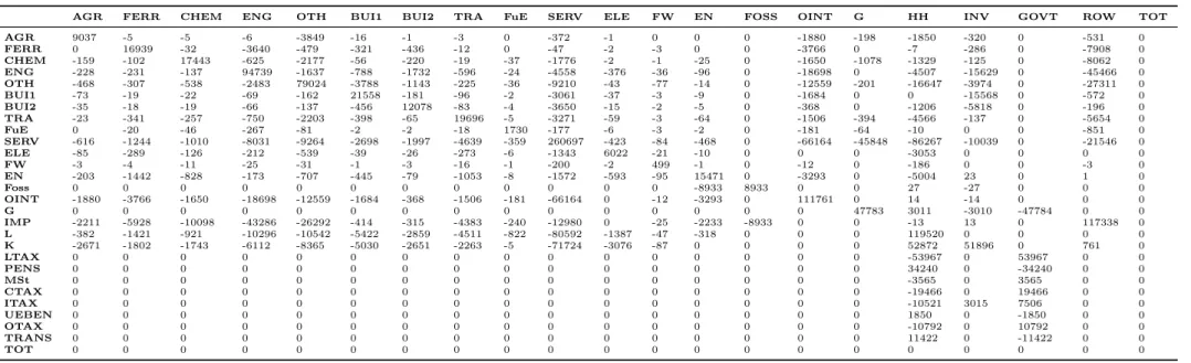
The old data set of MERCI (table 2.2) has been constructed for the benchmark year 2005, based on data by Statistics Austria mostly (I/O Tables), EU-SILC and Labour Force Survey, and has been updated to the year 2008 for DEFINE. This type of SAM is called a Micro Consistent Matrix (MCM ), which has the following distinguishing features:

Firstly, the data are arranged in such a way that inputs into production/expenditures by the producing sector enter the matrix with a negative sign , while output/revenues of producing sectors enter the matrix with a positive sign . Thus, the zero profit conditions (total costs for production equal total revenues from production) for the production sectors are depicted in the matrix by the column entries , where inputs and outputs have to be equal, thus sum up to zero.

Similarly, for the row entries , consumers’, or households’, expenditures on consumption of goods are denoted with a negative sign , whereas income/revenue is depicted with a positive sign . Thus, market clearance is represented in the benchmark data set by expenditures/consumption equaling revenues/income. The market clearance condition is thus ensured by the row entries summing up to zero.

All entries in the SAM are in Mio Euro. Each column in the SAM represents a sector or

agent. Concerning the representative and government agent, respectively, the positive entries

2.2 Model Implementation and Application to Austria

are income from labor, capital or transfers (taxes), the negative entries are expenditures for consumption goods or taxes (transfers). The ROW (rest of world) agent receives income from domestic imports; the difference of imports and exports (current account) enters as additional capital good available to the sectors for production.

Each row in the SAM represents a good, factor or tax/transfer payment. The positive entry

in each row represents the total produced quantity of the good, the negative entries stand for

the use of the good in the different sectors or by the different agents.

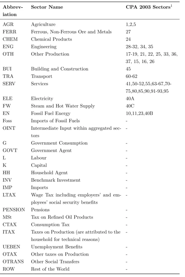
Table 2.1: Sectors of the MCM - SAM before DEFINE

Abbrev- iation

Sector Name CPA 2003 Sectors

AGR Agriculture 1,2,5

FERR Ferrous, Non-Ferrous Ore and Metals 27

CHEM Chemical Products 24

ENG Engineering 28-32, 34, 35

OTH Other Production 17-19, 21, 22, 25, 33, 36,

37, 15, 16, 26

BUI Building and Construction 45

TRA Transport 60-62

SERV Services 41,50-52,55,63-67,70-

75,80,85,90,91-93,95

ELE Electricity 40A

FW Steam and Hot Water Supply 40C

EN Fossil Fuel Energy 10,11,23,40B

Foss Imports of Fossil Fuels -

OINT Intermediate Input within aggregated sec- tors

-

G Government Consumption -

GOVT Government Agent -

L Labour -

K Capital -

HH Household Agent -

INV Benchmark Investment -

IMP Imports -

LTAX Wage Tax including employers’ and em- ployees’ social security benefits

-

PENSION Pensions -

MSt Tax on Refined Oil Products -

CTAX Consumption Tax -

ITAX Taxes on Production (are attributed to the household for technical reasons)

-

UEBEN Unemployment Benefits -

OTAX Other taxes on Production -

OTRANS Other Social Transfers -

ROW Rest of the World -

1 These Sector classifications refer to the CPA classification of Statistik Austria in the input-output tables of 2005. The input-output tables can be obtained from http://www.statistik.at/web_en/dynamic/statistics/national_accounts/input_output_

statistics/publikationen?id=&webcat=358&nodeId=1096&frag=3&listid=358. Last