Research Collection
Bachelor Thesis
3D geological model of a shear zone conditioned on geophysical data and geological observations
Author(s):
Hediger, Roman Publication Date:
2020-06
Permanent Link:
https://doi.org/10.3929/ethz-b-000455004
Rights / License:
In Copyright - Non-Commercial Use Permitted
This page was generated automatically upon download from the ETH Zurich Research Collection. For more information please consult the Terms of use.
3D geological model of a shear zone conditioned on geophysical data and
geological observations
to obtain the academic degree
Bachelor in Earth Sciences
submitted to the Department of Earth Sciences at ETH Zurich Institute of Geophysics
supervised by
Dr., Alexis Shakas, ETH Zürich, Institute of Geophysics, Zurich Prof. Dr., Hansruedi Maurer, ETH Zürich, Institute of Geophysics, Zurich
Dr., Hannes Krietsch, ILF Consulting Engineers AG, Zurich
submitted by Roman Hediger
15-935-646 at
Wil, 30.06.2020
A considerable amount of research is currently conducted in Switzerland in the field of geothermal energy. That is because the Swiss Energy Strategy 2050 aims to increase the percentage of them in energy production to 7% of projected energy demand. One of these places where research is done is the Bedretto Underground Laboratory for Geoenergies (BULG) in Ticino. The BULG is a research facility in the Bedretto Tunnel surrounded by Rotondo-granite, starting at 2 km (Tunnel Meter TM2000) into the 5 km long tunnel. During three different drillings (boreholes CB1-CB3, lengths: 300m, 220m, 190m) in the southwestern wall, enhanced water outflow from the boreholes was noted, when intersecting a shear zone called Characterization Borehole Shear Zone (CBSZ). This indicates that CBSZ has a high hydraulic permeability. A permeable structure in the subsurface is of high interest concerning geothermal reservoir research. However, before this zone can be examined more precisely, its course in the underground must be determined. In this thesis, firstly, a model of CBSZ is developed; secondly, the intersection of this shear zone with the tunnel is deduced, and thirdly the history of its origin is investigated. The modeling tool used is called Gridfit and approximates a best-fitting surface between all inserted data points. Therefore, optical and acoustic borehole logging data sets and ground-penetrating radar images of all CB boreholes, as well as geological drill core descriptions, are available. From the logging data, the orientation of CBSZ in the boreholes is determined. Whereas from the GPR images, the course of the shear zone further away from the CB’s, is deduced. A combination of these two data sets unites regionally exact logging measurements as well as slightly less accurate GPR data sets of the shear zones’ course in the granite. This data are sequentially transferred to Gridfit, which constructs a more accurate model with each additional information. The resulting model has a slightly curved fracture surface towards the tunnel and is now compared with known fractures from the tunnel. Thus it follows that CBSZ is most likely the structure TM1986 from the Bedretto Tunnel. From the history of its origin, it can be concluded that the shear zone was initially formed under ductile conditions with temperatures over 250−350◦C prevailing. These are conditions that are reached in depths of more than 10-15 km. Afterwards, there was an uplift of the Rotondo-granite and an associated cooling of the rock. Later the shear zone was reactivated again but deformed brittle due to the relatively low temperatures. This brittle deformation is very likely to be the origin of the high porosity that CBSZ has today. An important application of these findings is that it is now possible to predict how deep further drillings have to be planned to encounter CBSZ. Furthermore, based on them, more research around this shear zone can now be initiated.
Abstract i
1 Introduction 1
1.1 Overview . . . 1
1.2 Geological setting . . . 2
1.3 Objectives . . . 3
2 Data 5 2.1 General data overview . . . 5
2.2 Acoustic and optical logging . . . 5
2.2.1 Acoustic method . . . 5
2.2.2 Optical method . . . 6
2.2.3 Application in model . . . 7
2.3 Borehole GPR. . . 8
2.3.1 Principle . . . 8
2.3.2 Data from survey . . . 8
2.3.3 Processing steps . . . 8
2.3.4 Application in model . . . 11
2.4 Tunnel information . . . 11
3 Methods 13 3.1 General modelling approach . . . 13
3.2 MATLAB Tools . . . 13
3.2.1 GPR fracture picking and orientation in 3D . . . 13
3.2.2 Gridfit. . . 15
3.3 Characteristic properties of the model . . . 17
3.4 Velocity model . . . 18
3.5 Origin of CBSZ . . . 19
4 Results 21 4.1 Logging model . . . 21
4.2 Combined logging and GPR models . . . 22
4.2.1 Model M1 . . . 23
4.2.2 Model M2 . . . 24
4.4.1 Model M1976 . . . 26 4.4.2 Model M1986 . . . 28 4.4.3 Model M1994 . . . 29
5 Discussion 31
5.1 Formation process of CBSZ . . . 31 5.2 CBSZ Modeling. . . 32
6 Conclusion 35
7 Acknowledgements 37
Bibliography 39
List of Figures 43
List of Tables 45
A Appendix 47
A.1 Logging data . . . 47 A.2 GPR data . . . 47
1 Introduction
1.1 Overview
A considerable amount of research is currently being conducted in Switzerland in the field of geothermal energy. That is because the Swiss Energy Strategy 2050 aims to increase the percentage of them in energy production to 7% of projected energy demand. One of these places where research is done is the Bedretto Underground Laboratory for Geoenergies (BULG) in Ticino. The BULG is a research facility in the Bedretto Tunnel operated by ETH Zurich and many other research institutions and private companies.
Originally built as an intermediate attack for the Furka Basis Tunnel in 1982, it was later converted into a research facility on a length of about 100 meters. The laboratory starts at Tunnel Meter 2000 (TM2000) into the 5 km long tunnel (see Figure1). Due to the unique geological conditions around the laboratory, namely the homogeneous and fractured Rotondo-granite (Keller and Schneider,1982), this is a unique place to study sustainable and efficient geothermal reservoir creation. Briefly explained, the petrothermal energy production works as follows: A cold fluid (mainly water) is lowered in boreholes and pumped into the rock. Then it circulates in the rock to extract heat from it and serves thereby as a heat exchanger medium. The heated fluid is then pumped back up to the surface, where the stored heat can be used. The hot fluid can either be utilized to heat buildings directly in winter or indirectly to produce electricity (e.g.Swiss Seismological Service,2016). The many fractures around the BULG and its location provide optimal conditions for hydraulic stimulation reservoir creation experiments with a subsequent examination of the fluid circulation in the reservoir. Since the laboratory is overburden by one kilometre of granite, no kilometre deep drillings are necessary to get to the region of interest.
Research can, therefore, be conducted very efficiently here.
In summer 2019, three down-dipping holes, called CB1 to CB3 (Characterization Boreholes 1-3), (Table 1), were drilled into the southwestern wall of the BULG. During drilling, the water flow considerably increased when hitting a specific fault zone. This fault zone was encountered in all three drill holes. This, together with the increased water flow, indicates that this structure has a vast expansion in space and has enhanced hydraulic permeability. Structures like these are of high interest for geothermal research because exactly such highly permeable structures are needed to allow the fluid to circulate into the warm host rock. For further planned drillings in the southwest wall of the tunnel, it is essential to know the course of this fault zone. There were essentially two approaches for this: In a study made byShakas et al.
(2020), they selected this structure to model its trajectory and thus also their potential intersection with the tunnel. Here the fault zone is assumed to be a planar feature. According to their studies, the model intersects the tunnel 50 meters before the BULG, which corresponds to TM1950. Because the fault zone
Figure 1: The position of the BULG (red) in the 5 km long Bedretto Tunnel is visible on this figure as well as the geological units around it. The laboratory is located under a 1 km thick rock cover, embedded in Rotondo-granite.
The picture is modified fromKeller and Schneider(1982).
shows indications for shear dislocation, it will henceforth be called a shear zone. Another approach by Castilla et al.(2020) assumes that this shear zone is of curved appearance, which would make the 3D interpolation more complex. This is also a realistic scenario because shear zones with a curvature occur in nature as examined by, e.g.,Vendeville(1991).
After the three CB boreholes were drilled, several geophysical surveys such as optical and acoustic tele- viewer logging (OTV & ATV) as well as ground penetrating radar (GPR) (Section2) were carried out.
Furthermore, orientation measurements (coordinates, strike and dip) exist from all visible fault zones in the tunnel (Jordan,2019). Among othersBrixel et al.(2020a,b) showed the hydraulic properties inside a shear zone can be very heterogeneously distributed. Within this thesis, the shear zone in question is in- terpolated, based on a-priori geological information and geophysical observations. For the interpolation, it was considered that the shear zone does not need to have significant outflow at the tunnel intersection.
This shear zone, which from now on will be called CBSZ (Characterization Borehole Shear Zone), is visible, especially in the sampled GPR data.
1.2 Geological setting
The Bedretto Tunnel is a straight tunnel with an azimuth of 317N. Different lithologies are crossed when going from southeast to northwest. The first 1100 TM are gneisses and amphibolites of different rock series. This is followed by a sharp transition to the Rotondo-granite, which continues to the end of the tunnel (Keller and Schneider,1982). The 100-meter long BULG is located in this last formation,
which intruded 293-295 million years ago (Sergeev and Steiger,1995) and builds up a part of the so- called Gotthard Massif (Keller and Schneider,1982). It has thus witnessed the formation of the Alpine mountains and the associated uplift of the Gotthard Massif (Herwegh et al.,2017).
This granitic body consists of quartz, plagioclase, feldspar, and small amounts of sericite and biotite.
The granite is equigranular, massive, and in some places also porphyric (Hafner,1958). In the area of investigation around the BULG, it is crossed by four different families of fractures or clefts (Castilla et al.,2020). Many of these fractures show an inflow of water or are at least wet. Furthermore, there are several locations, especially between the southern entrance and the BULG, with an inflow rate of more than 1 L/s depending on the season (Jordan,2019).
1.3 Objectives
All mentioned geophysical and geological information together allow creating a new model of CBSZ, based on more data than ever before. Besides modeling, the development history of CBSZ also plays a vital role in current research. It is essential to understand how such presumably very porous zones were formed. An interpretation of the educational history of CBSZ is, therefore, also part of this thesis. The objectives of this thesis are summarized below:
1. Building a 3D geological model of CBSZ conditioned on a combination of different geophysi- cal data like GPR, optic and acoustic borehole logging, as well as tunnel observations and other geological information. In contrast to the study fromShakas et al.(2020), the model allows the surface to curve.
2. Determine the most likely intersection of CBSZ with the tunnel based on the best model achieved from objective 1. For this purpose, the mapped fault zones from the tunnel are compared with the most consistent modeled surface.
3. Concluding the formation process of CBSZ and the circumstances prevailing then, such as tem- perature and depth. Based on the model and the geological information from the drill cores and the tunnel.
2 Data
2.1 General data overview
For this thesis, both geophysical and geological data sets are available. In addition to local and very precise optical and acoustic logging measurements (Section2.2), borehole GPR data from the whole structure are also available (Section2.3). These data collected in the boreholes far away from the BULG are combined with mapping measurements of fault zones in the Bedretto Tunnel. For this purpose, the data fromJordan (2019), who has mapped and described every fault zone in the first 2.25 km of the tunnel, are used. Furthermore, detailed geological descriptions of CBSZ are available in the report of Castilla et al.(2020), which will provide information on the history of its formation.
Because CBSZ-modelling is mainly based on data collected in the three drill holes CB1-CB3, their most important properties are summarized in Table1. Furthermore, all applied geophysical measuring methods per borehole are listed in Table2, since not all of them were used in each drill hole.
Table 1: A summary of the properties of the three drill holes is given in this table. The down-dip is specified concerning the horizontal.
length (m) down-dip CBSZ intersection (m)
CB1 300 45◦ 143
CB2 220 50◦ 130
CB3 190 40◦ 119
Table 2: An overview of the geophysical measurement methods used in boreholes CB1-CB3 (Shakas et al.,2020).
CB1 CB2 CB3
GPR 100 MHz 3 3 3
Optical logging 3 8 3
Acoustic logging 3 3 8
2.2 Acoustic and optical logging 2.2.1 Acoustic method
CB1 and CB2 were assessed with acoustic televiewer logging (ATV). Therefore, ultrasound with a pen- etration depth of 1-2 cm is used. For this purpose, a logging antenna with a transmitter and a receiver is lowered or pulled up the borehole. ATV has two measurement parameters. The first is the amplitude.
Thereby, different strengths of the signal reflection at the borehole wall are recorded, which represent a rough correlation with the material properties encountered. This makes fractures and other structures visible because they reflect another amount of energy than the relatively smooth borehole wall. The second parameter measured is the travel time. This value can provide information on opening width or
shear offset of fractures in the borehole (Wonik and Olea,2007). The mean CBSZ-orientation can later be determined from these ATV images. Furthermore, with an adapted distance measuring system, the exact position of these structures inside the boreholes can be deduced. Figure2 shows inter alia two processed images of the acoustic logging survey in CB1.
2.2.2 Optical method
All boreholes under investigation show a continuous outflow of clear water; these are optimal conditions to ensure good data quality for optical televiewer logging. During measurement, the camera continuously records as it is pulled up the boreholes (Wonik and Olea,2007). From those images, an evaluation with respect to the borehole wall can be made. This method delivered together with a direction and distance measuring system, the exact position, and orientation of CBSZ intersections in CB1 and CB3. This provides a complementary data set with respect to the ATV. An optical logging image from CBSZ in CB1 is inter alia shown in Figure2.
Figure 2: The image on the left shows a representation of travel time, and the one in the middle shows one of amplitude from ATV measurements inside CB1. Colour differences indicate inhomogeneities in the borehole wall.
On the right side, the corresponding optical logging picture is shown (Castilla et al.,2020). All fractures are visible as sinusoids (marked black). That is an effect of the 3D circular borehole wall illustrated on 2D. Now strike and dip of the suspected fracture (CBSZ in CB1) can be determined.
2.2.3 Application in model
Logging information in each borehole is very accurate. However, this is very local information and can only be used as an approximation of the shear zone very close to the boreholes. The logging orientation measurement is imported to the surface fitting program Gridfit as oriented circles with a diameter of one meter each (Section3.2.2). Each of them consists of 100 individual data points, representing the mea- sured strike and dip of CBSZ. This chosen circle’s diameter is small enough compared to the borehole, so that the information is reliable, and also far enough away that Gridfit does not take it as one single data point. If that happened, the logging orientation would not provide useful information for the CBSZ model.
2.3 Borehole GPR 2.3.1 Principle
GPR is a widely used instrument to probe the ground, especially for determining its geological properties.
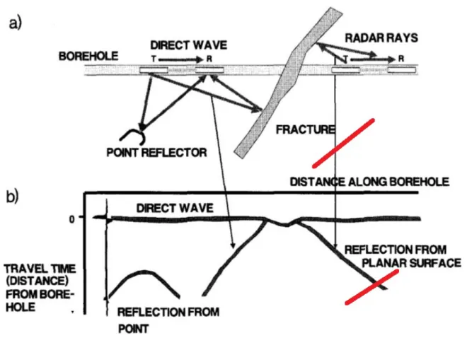
It sends high-frequency electromagnetic waves into the ground and receives the reflected signal. This property is also one of the most significant advantages of this technique. It is a non-destructive method (Annan, 2009). For borehole GPR, however, this is not entirely true for the borehole GPR-survey in the Bedretto Tunnel, as holes had to be drilled into the granite first. Afterwards, the instrument makes its measurements independently while it is usually continuously pulled up the borehole. A distinctive feature of this method is that data is captured in 3D, but displayed in 2D. That can lead to azimuthal ambiguity, which causes the fractures intersecting the borehole to be displayed as V-shape in the GPR image. This means furthermore that it does not necessarily have to be the case that structures which lie on top of each other in the picture, actually intersect. For example, since they can be on different sides of the borehole (see Figure3).
GPR is well suited to detect structures in bedrock, especially water-filled fractures, as the CBSZ is probably one. Since water and granite have different electrical properties, their interface produces a sharp reflection (Slater and Comas,2009). Before working with the GPR data, some processing steps must first be completed (Section2.3.3).
2.3.2 Data from survey
For further CBSZ-modelling, GPR images collected with a frequency of 100 MHz are used. They have a sufficiently high resolution and penetration depth for further work.
2.3.3 Processing steps
It is important not to produce unrealistic artefacts in the data during processing. The following steps were only used to remove unwanted signals from the data, such as the first reflection from the borehole wall (first break) or random noise. Furthermore, known measurement weaknesses such as the Wow-effect are removed. The following sections show which steps were carried out on the data. In Figure5 are the influences of the remove window mean and the time gain processing step shown. The bottom image also corresponds to the final image used for modelling.
Remove conductor pipe and time-zero correction: Variations in the distance between the receiver and the borehole wall, as well as thermal drift or electronic instability of the measuring device, can lead to disturbances in the data (Olhoeft,2000). As a result, the single traces do not start at a common time-
Figure 3: This image modified fromOlsson et al.(1992) shows the effect of azimuthal ambiguity. This means that a fracture that intersects the borehole produces a kind of V-shape in the final image. Another effect is shown in red. The grey and the red fracture are on different sides of the borehole and do not intersect with each other. But in the final picture, exactly this impression is produced.
zero point. Therefore a correction is needed, which takes, e.g., the first breakpoint of the airwave or the first negative peak in the data and sets them to time equals zero point (Cassidy,2009).
The last 300 traces are removed during data processing. These reflections are from the metal conductor pipe, which does not allow to see anything in the rock. Leaving them would disturb the further processing steps.
High-pass filter: Received frequencies under 40 MHz are removed. All higher frequencies are al- lowed. This process removes the low-frequency noise, whereby the best and most detailed GPR images are observed. It is always important to keep in mind that filtering can also remove wanted signals and, therefore, relevant information. That is not the case by applying the mentioned filtering window since the final images contain all essential structures for the modelling of CBSZ.
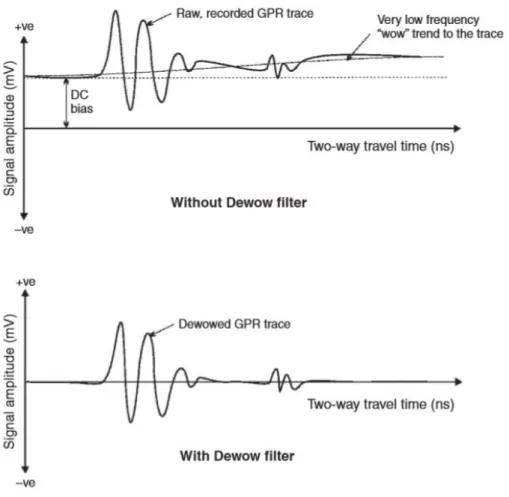
Dewow filtering: The dewow filtering aims to remove the initial direct current (DC) signal, also called the DC bias (see Figure4), and the following decay of the low-frequency signal content (Dougherty
et al.,1994). The low-frequency signal trend is also called "Wow" and arises from a saturation of the received signal, e.g. caused by early arrivals like a ground or airwave (Annan,1993).
Figure 4: This figure shows the influence of dewow filtering. By applying dewow filtering, the low-frequency content does not get lost (Cassidy,2009).
Remove window mean: This custom made filter removes the mean over a running window. That smoothes the data and is an effective way to remove ringing effects as well as the signal of the direct wave.
Time gain: Due to spherical spreading, attenuation and scattering of the transmitted energy, signals with a late arrival time (t) at the receiver are very week compared to others from closer to the borehole (Annan, 2009). With an exponential time gain function (tgain), these signals are amplified and made visible. Therefore, the result of the time gain function is multiplied by the signal strength. The exponent chosen during the borehole GPR processing for all scenarios was: gain = 2.5. The best results were achieved when using this value. The applied time gain is a nonlinear function, and hence, different results can occur if the processing is not carried out in the same order as described here.
Figure 5: (a) The raw data, including the last 300 traces, which are removed for any further steps, are shown here. The effect of the processing steps remove window mean (b) and time gain (c) are shown. The other three processing steps were also applied here in the same order as described. However, since there is no influence on the output visible to the naked eye, no representation was made.
2.3.4 Application in model
GPR provides information far from the borehole, but this data is much less accurate than the CBSZ orientations from the local logging measurements. Therefore, two complementary data are included in the modelling. The GPR paths are recorded with a custom made MATLAB program and later oriented in space (Section3.2.1). Therefore, the path is divided into many data points, which are later passed to the Gridfit function (Section3.2.2).
2.4 Tunnel information
Jordan(2019) mapped fractures and shear zones intersecting the tunnel. Every structure is described in terms of orientation (strike and dip), coordinates, tunnel meters (location along the tunnel with TM0 being the tunnel entrance and TM2000 the lab entrance) and geological properties. Because CBSZ
presumably is likely to be hydraulically conductive, preferably moist or water-bearing structures are included in the modelling. They also should intersect the tunnel in the area between approx. TM1950 and TM2000 as previous studies suggest (Shakas et al.,2020,Castilla et al.,2020).
There are mainly five structures, which after a closer look apply to these descriptions. Their position in TM is 1972, 1976, 1986, 1994 and 2001. Unfortunately, the noted coordinates from the fault zone at TM2001 are not correct, because they plot very far away from this point. Furthermore, the TM1972 measurement cannot be used either, as it plots about 7 meters away from this point. However, the three fault zones with the correct positions will be considered in the final interpretation. They are at the end given to Gridfit. In this way, it can be determined which of these fault zones best fits the model based on GPR and logging data. Fitting means inter alia that it does not change the model to an unlikely scenario with bumps, holes or waves in it. The further conditions are summarized in Section3.3.
3 Methods
3.1 General modelling approach
Three different data sets are used to develop the model. Some of the information was gathered in the three boreholes CB1-CB3. Others were collected in the tunnel while studying all visible structures in the wall. These data sets are:
1. Acoustic and optical orientation borehole logging data.
2. Borehole GPR data from all three boreholes.
3. Logging information of all structures visible in the tunnel (Jordan,2019).
4. Precise geological descriptions of borehole cores.
ETH assessed all used borehole logging and GPR datasets. The geological descriptions of the drill cores are taken from the report ofCastilla et al.(2020).
The modelling approach is as follows: More information is added stepwise. This means that the logging information from the boreholes comes first (Section2.2.3). Then a model is generated, and when this is finished, data set two is added and so on. The last data set is the tunnel measurements; their application in the model is described in Section2.4. This approach allows for noticing the influence of each step to determine later what had the most impact. Also, it allows excluding false or inaccurate data sets since they would influence the model in an illogical manner (Section3.3). In this way, an increasingly accurate model can be generated. Besides modelling, one of the main objectives is to hypothesise the most likely intersection of the CBSZ with the Bedretto Tunnel. This decision will be based on the built model and also all available geological information (Section1.2).
The following chapters describe the methods used to process the data. Furthermore, the functionalities of the used modeller programs are explained.
3.2 MATLAB Tools
3.2.1 GPR fracture picking and orientation in 3D
After complete processing of the 100 MHz GPR borehole data (Section2.3.3), three images of the bore- holes’ environment are available for the path picking. Therefore, a specific MATLAB program is used, which exports the paths of CBSZ to use it for modelling later. This program allows to manually pick the course of CBSZ in each of the three GPR images. Since it is known at what depth the shear zone
intersects the boreholes, CBSZ can always be identified in the pictures.
Used GPR paths and path picking
GPR-up paths are the parts of CBSZ between the tunnel and the borehole intersection. The GPR-down paths are those that start at the borehole intersection and then lead away from the tunnel. An example from CB1 is provided in Figure 8. GPR-up and down paths can be determined from each of the three GPR images. Using a custom made MATLAB script, the paths are marked by hand and then saved as vectors. They are later named accordingly. If the paths originate from the GPR image of CB1, they are called CB1-up path and CB1-down path and so on. The second part of the name indicates the place where they lead to. If this part is, e.g. "to CB2", it means that the path will meet this borehole on its way.
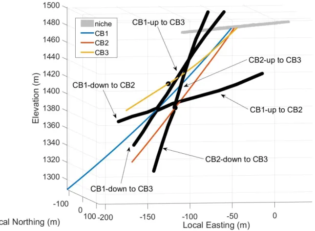
For the subsequent modelling, the following three up-paths and their corresponding down-paths are used:
(see Figure7):
1. CB1-up path to CB2 2. CB1-up path to CB3 3. CB2-up path to CB3
Only these enumerated up-paths are used because just they can be orientated in the three-dimensional space afterwards. This is for the following reason, only they intersect one of the other two boreholes.
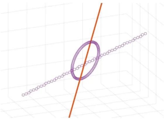
However, this fact makes orientation possible because then two points of the path are known, namely the starting point and a point where the path goes through. This also means that the GPR image of CB3 does not represent use for modelling, as the CB3-up path does not intersect any other borehole. In the GPR-picture (see Figure26) it looks like this, but in reality CB3-up path and CB2, CB1 are on different sides of the borehole (see Figure6). This effect is also described in Figure3. Furthermore, it is not possible to orient the path CB2-up to CB1. This is due to the same effect. After picking the paths, they get now oriented in space.
Orientation of picked paths
The orientations of the picked paths in space still need to be determined. Since it is known that CB1-up to CB2 intersects CB2 and CB1-up to CB3 intersects CB3, our path must now do the same. Therefore two paths are started from CB1-CBSZ intersection point (at 143m). One has to intersect CB2 (CB1-up to CB2) and the other CB3 (CB1-up to CB3) (see Figure7). With a custom made MATLAB script, the picked paths can be moved into this position by manually choosing the right angle. The path itself can be rotated 360 degrees around the starting point at the borehole-CBSZ intersection, its course itself is
Figure 6: View of the situation from below. Since the CB3-up path and the other two boreholes are on opposite sides, they do not intersect although it looks like this on the GPR image from CB3 (see Figure26).
not changed. Logically, there are 180 degrees angle difference between the up and the corresponding down path. So, the down paths can afterwards be oriented easily. The same procedure can be used for the CB2-up path to CB3.
It is also immediately obvious that the GPR data and the logging data do not match exactly; there is a distance between them of several meters (see Figure7). After the complete orientation in space is done, this inaccuracy is further addressed in Section3.4.
.
3.2.2 Gridfit
Gridfit takes several coordinate points in 3D and approximates a best-fitting surface between them. In this case these are the data points from borehole logging, GPR and also from tunnel measurements. The inserted data points pull the surface towards them, but the applied bending rigidity of the model works against it. Therefore, the surface will not exactly intersect all given coordinates. What happens instead is
Figure 7: The two CB1-up paths and corresponding CB1-down paths are labeled here as well as the CB2-up to CB3 and down paths. Furthermore, the Bedretto Tunnel here called niche, and the trajectories of the three boreholes CB1-3 are shown.
that an approximation of the most likely CBSZ course is made. A strength of Gridfit is that it can handle noisy and replicated data because of these described properties. Because the surface has a tendency to become planar when no data points are nearby, it is crucial to have information from the whole structure under investigation at least partially (D’Errico,2006). This precondition is fulfilled since the used data (Section3.1) covers nearly the whole course of CBSZ. Furthermore, care is always taken to ensure that the model is only calculated in a range as large as absolutely necessary. So, the model will end just after the tunnel because there is no information about the further course of CBSZ beyond this point. The strength of rigidity can be chosen. This value will be adjusted after all data points are at its final position as described in Sections2.2.3,3.2.1. A good value for the rigidity is reached when the final surface has no unnatural waves, bends, bumps or holes in it. Then gridfit produces a smooth shaped model of CBSZ.
Figure 8: GPR image from CB1 with the labelled CB1-up and CB1-down paths (red) and the intersections from CBSZ with the three boreholes are shown here. The paths are not yet marked with the addition "to CB..." because they are not yet oriented. The CB1-up path starts at zero meters distance along with CB1, which means this path begins near the tunnel. The path ends at the intersection of CB1 and CBSZ. At this point, the CB1-down path starts and in the following distances itself more and more from the tunnel.
3.3 Characteristic properties of the model
Each model made is critically examined at the end and rejected if there are any discrepancies. The main points that are taken into account are summarised in the following list:
1. Are there any unnatural bends, waves or holes into the modeled surface, which can not be corrected with a moderate increase of the rigidity value from Gridfit tool?
2. Do the GPR paths start or intersect at the same point as the borehole logging data indicate? Always considering that GPR data itself and the manual path-picking (Section 3.2.1) are associated with uncertainties estimated to be a few meters. Large distances between them (see Figure 9a) are corrected by changing the velocity model (Section3.4).
3. Does the model stay close to the implemented data points, or does it deviate from them? This occurs if the range in which the model was calculated is too narrow. In this case, the model range must be adjusted.
4. Since earlier studies assume that CBSZ is curved (Castilla et al.,2020), attention is also paid to a curved appearance of the model. This is especially important from the implementation of the GPR data onwards because the model tends to become planar far away from the local logging data.
3.4 Velocity model
The y-axis of the GPR images (see Figures 8, 25, 26) denotes the radial distance in meters from the borehole. That value is determined by multiplying the travel time of the GPR signal with the average velocity of the signal in the host medium. This value has been measured as v = 0.1279 m/ns from independent laboratory measurements on samples from the borehole cores. Although this is the correct velocity, there is an offset of several meters between the borehole logging and the GPR data. This is clearly visible, for example, at the intersection point of CB2 and CBSZ (see Figures9a,7). Here, the two data sets would have coincided. They do not have to fit exactly since GPR data are subject to uncertainties. But the actual distance of more than 10 meters (CB2 & CB3) is too large. Therefore, after modelling with the correct velocity, another model is created with an adapted velocity. This reduces the inaccuracies in the data. The new velocity is determined in with the following approach: The velocity is increased with 0.005 m/ns steps until the distance between the different data sets becomes smallest.
The distance between borehole logging and GPR data in the uncorrected model in CB2 is around 11 meters (see Figure 9a). After the implementation of the corrected velocity, v = 0.200 m/ns, the two data sets coincide very precisely (see Figure9b). Furthermore, the distance in CB3 is reduced to about 1.5 meters from more than 10 meters before. When trying to increase the velocity even further, the distance increased again. For the CB2-up path to CB3, no correction velocity could be found to bring the distance to a reasonable level. Therefore this path is omitted in the corrected model. Since this correction velocity is much higher than the velocity actually measured, this value must be regarded merely as a kind of correction factor, which takes into account the inaccuracies in the measurements and possible non- isotropic rock conditions. As a result of the new calculated paths, some orientation azimuths (Section 3.2.1) need to be changed, but only by a few degrees.
(a) In the boxes, the coordinates of the intersection from logging and GPR with CB2 are shown. The calculated distance between them is√
5.22+5.012+82= 10.8 me- ters.
(b) After the velocity correction, the offset between GPR and logging is almost zero at CB2 and the logging orien- tation matches very precisely to the GPR-path direction.
Figure 9: Uncorrected (left) and corrected (right) model between GPR and logging data. Shown on the example of the CB1-up path to CB2 at borehole CB2.
3.5 Origin of CBSZ
Any geological interpretation, regarding the geological origin of CBSZ, is done based on the drill cores from CB1-CB3. An overview of the found lithologies around CBSZ (suspected fracture) is provided in Figure10. The investigation will focus on lithologies and geological features occurring in all three cores. For the study of the origin of this shear zone, however, the adjoining areas are also included as the CBSZ formation may have also influenced them. There is no other direct geological information from this shear zone at the moment since it is not known where the tunnel intersection of CBSZ is and because no further core descriptions are available.
Figure 10: Geological drill core descriptions (CB1-3) modified fromCastilla et al.(2020). The suspected fracture is the CBSZ under investigation. The naming of the different geological sections is provided in the legend, and its thicknesses are visible in the figure as well.
4 Results
All subsequent models have passed the test according to the specified criteria (Section3.3). An exception are the logging model (see Figures11,12) and the combined logging and GPR model (see Figures13, 14), where no correction of the velocity has been made yet and the distances between GPR and logging data are large.
4.1 Logging model
The first model is only constrained by logging data from the boreholes (Section2.2). Its most essential properties are summarized in Table3. Although only these very regional data were implemented in the model, the surface shows even further away of the boreholes a slight curvature towards Bedretto Tunnel.
The modeled surface is visible in Figures11 and12as well as the intersection with the tunnel at Y = -13. This value corresponds to TM1987, and because the origin of Y-coordinates is located exactly at the beginning of BULG’s entrance, CSBZ crosses the niche (tunnel) 13 meters before its entrance. This entrance is recognizable by the thickening of the niche.
Figure 11: The Logging model from a slight top-down view is shown here (blue). The black circles are the implemented logging data around CB1-CB3. This first model shows a slightly curved appearance and intersects the niche at TM1987.
Figure 12: Second view of the logging model from NE (blue).
4.2 Combined logging and GPR models
Next, the six specific GPR paths (Section3.2.1) are added to the existing logging model. Two models were developed, the first based only on GPR data from CB1 (M1) (see Figures13,14), the second with all GPR data applied (M2) (see Figures15, 16). Furthermore, the main properties of M1 and M2 are shown in Table3.
Table 3: Overview of the data used for modelling and the most important properties of combined logging and GPR models (M1 & M2) and of the logging model are shown here. A tick means that all, a cross that no data of this type was used. The tunnel intersection gives the intersection in TM of the model and the tunnel.
logging M1 M2
Borehole logging 3 3 3
GPR 8 CB1 CB1,CB2
Tunnel information 8 8 8
Tunnel intersection TM1987 TM2008 TM1980
4.2.1 Model M1
Figure 13: Model M1 from a slight top-down view is shown here (blue). The tunnel intersection is at TM2008.
The black lines represent the GPR-paths.
Figure 14: Another view of model M1 from NE is provided here.
4.2.2 Model M2
Figure 15: Model M2 from a slight top-down view is shown here (blue). The black lines are the implemented GPR paths from CB1 and CB2. At TM1980, CBSZ intersects the tunnel.
Figure 16: Model M2 is shown here in a view from NE.
4.3 Velocity corrected, combined logging and GPR model
All models from here on are based on a corrected GPR velocity model (Section3.4), with an applied velocity of v = 0.2 m/ns. This correction does not have any influence on the borehole logging or tunnel measurements. For better differentiation, the surfaces are now coloured in green.
This corrected model (see Figures17, 18) was created without the GPR data from CB2 as it was not possible to correct it sufficiently. Its properties are summarized in Table4.
Table 4: Overview of the data used for modelling and the most important properties of the velocity corrected, combined logging and GPR model.
Borehole Logging 3
GPR CB1
Tunnel Information 8 Tunnel Intersection TM1978
Figure 17: The velocity corrected combined logging and GPR model from a top-down view is shown here (green).
In contrast to the previous models, the correction factor was applied.
Figure 18: The velocity corrected combined logging and GPR model from a NE-view is shown here.
4.4 Velocity corrected, combined logging, GPR and tunnel information models 4.4.1 Model M1976
This is the first model where all available data is implemented. Here the result with the tunnel mea- surement TM1976 is shown (see Figures 19, 20). Its most relevant characteristics are listed in Table 5.
Table 5: Overview of the data used for modelling and the most important properties of all velocity corrected, combined logging, GPR and tunnel information models. Tunnel information means the fault zone from the tunnel implemented in the corresponding model.
M1976 M1986 M1994
Borehole Logging 3 3 3
GPR CB1,CB2 CB1,CB2 CB1,CB2
Tunnel Information TM1976 TM1986 TM1994 Tunnel Intersection TM1978 TM1984 TM1995
Figure 19: Velocity corrected combined logging, GPR and tunnel information model TM1976 from a slight top- down view is shown here. The black circle in the Bedretto Tunnel marks the location and orientation of the implemented Tunnel Measurement TM1976.
Figure 20: Velocity corrected combined logging, GPR and tunnel information model M1976 from a NE-view.
4.4.2 Model M1986
This is the second model, where all available data is implemented. Here the result with the tunnel measurement TM1986 is shown (see Figures21,22). Its most relevant characteristics are listed in Table 5.
Figure 21: Velocity corrected combined logging, GPR and tunnel information model TM1986 from a slight top- down view is shown here.
Figure 22: Velocity corrected combined logging, GPR and tunnel information model M1986 from a NE-view.
4.4.3 Model M1994
This is the third and last model, where all available data is implemented. Here the result with the tunnel measurement TM1994 is shown (see Figures23,24). Its most relevant characteristics are listed in Table 5.
Figure 23: Velocity corrected combined logging, GPR and tunnel information model M1994 from a slight top- down view is shown here.
Figure 24: Velocity corrected combined logging, GPR and tunnel information model TM1994 from a NE-view.
5 Discussion
5.1 Formation process of CBSZ
Table 6 shows the occurrences of the most important geological units of CBSZ per borehole. Open rugose fractures and closed shear fractures do not occur everywhere and are not a distinguishing feature of CBSZ. Overall, the shear zone and its surroundings have four primary characteristics: foliated zones, gneiss texture zones, mylonite, and also porous zones. Especially the presence of mylonite in or nearby all three CBSZ-borehole intersections delivers information about its formation process. The formation of mylonite is a clear sign for a ductile deformation of the granite (Koch and Masch,1992,Simpson, 1985,Lützenkirchen and Loew,2011). Therefore, temperatures over 250−350◦C are necessary. These are conditions which are reached in depths of more than 10-15 km (Sibson,1977). Lützenkirchen and Loew(2011) stated that also a brittle deformation in Rotondo-Granite took place starting at temperatures slightly over 300◦C.
Table 6: Overview about the found geological units in and around each known section of CBSZ from boreholes CB1-3. The missing/broken core parts are ignored. A tick means this unit is found in the core, and a cross means the opposite. (F. Fracture; Z. Zone).
Closed Shear F. Open Rugose F. Foliated Z. Gneiss Texture Z. Mylonite Porous Z.
CB1 3 3 3 3 3 3
CB2 8 3 3 3 3 3
CB3 3 8 3 3 3 3
Based on this information, a possible history of formation for CBSZ is stated:
About 300 million years ago, an intrusion formed the Rotondo-granite. Later, the formation of several fractures, fault and also of the CBSZ took place. Many of these structures were built in ductile conditions, and so was CBSZ. This is evident from the mylonite encountered in all three drill holes. It occurs either in or just beside the suspected shear zone. Therefore temperatures above250−300◦C and a depth of more than 10-15 km prevailed at that time. Thereafter, the Rotondo-granite has continued to approach the earth’s surface through erosion and uplift.
The reason why CBSZ is today a fascinating structure for research is, however, its high hydraulic con- ductivity. The following hypothesis deals with the further development of this structure.
During the uplift of the rock, it cooled down and left the ductile deformation area. At temperatures below approx. 300 degrees brittle deformation sets in. Such processes have been detected in investigations on other fractures in the Bedretto Tunnel. It is therefore conceivable that after the ductile formation, brittle
processes also contributed to the present CBSZ. A characteristic feature are the porous zones in and around CBSZ. They were also encountered in all drilling. Furthermore, there is evidence that CBSZ is highly hydraulically conductive over large distances. These cracks and voids in the rock, where water flows through these days, were probably only formed during this second phase. Thus, the formation of these porous zones either occurred immediately after the ductile deformation at the transition to brittle, or CBSZ was later reactivated by tectonic events. Only a relative age sequence can be determined from the investigations. The absolute age at which these processes or this process took place cannot be determined.
5.2 CBSZ Modeling
The first model based on the borehole logging data can only be used as a first estimation of CBSZ’s course. The information is still too local to provide a reliable model far away from the boreholes. How- ever, this model is already in conflict with the planar model of Shakas et al.(2020), which predicts a tunnel intersection at TM1950. After completely adding the uncorrected GPR paths there is no conclu- sive picture of the tunnel intersection of CBSZ. However, the original assumption that the shear zone has a curved appearance can be confirmed. Such a shear zone shape can also be found in nature at other locations as stated byVendeville(1991).
The GPR paths in the uncorrected models are still subject to great uncertainties. This is especially evident in the fact that the borehole logging data and the GPR paths in the drill holes do not match. That could be solved by correcting the velocity model, which results in a slightly less curved CBSZ surface and a tunnel intersection further away from the BULG. Now, several fault zones visible in the tunnel can still be considered as CBSZ. With the implementation of different tunnel measurements of Jordan(2019), the model was completed and the CBSZ candidates were investigated in detail. As a consequence, the model TM1994 and therefore, fault zone TM1994 is not the tunnel intersection sought, because CBSZ would have to make an extreme kink on the side in the last meters before the tunnel, which is unrealistic considering the smooth previous course of the shear zone.
A closer look at the corrected combined logging and GPR model shows a tunnel intersection at TM1978.
The insertion of the tunnel measurement TM1976 in that model has a negligible effect on the CBSZ surface at the tunnel of less than one meter whereas TM1986 shifts the tunnel intersection by more than five meters towards the BULG. What stands out in both models is the relatively sharp bend above the tunnel, which is less distinctive in the TM1986 model. Such a strong bend is unlikely when the previous
course of the model is considered. Due to the less sharp bending, TM1986 is to be preferred purely from the model compared to TM1976 as CBSZ. This is consistent with the study byCastilla et al.(2020).
However, the difference is not significant enough to exclude TM1976.
Jordan(2019) noted water outflow of more than 1 L/s at TM1986 compared to just dripping water at TM1976. The increased outflow of water during drilling when reaching CBSZ and the formation of this shear zone indicates that it is water-bearing and porous. Therefore, from this point of view, it is very likely that TM1986 is the CBSZ we are looking for. However, even this is not conclusive evidence, since Brixel et al.(2020a,b) has shown that properties such as water flow can change significantly within a shear zone. Therefore, it is also possible that no or minimal water outflow can be seen in the tunnel, which fits TM1976.
So, the following findings are stated:
1. The most coherent model of CBSZ is the TM1986 model.
2. The most likely intersection of CBSZ with the Bedretto Tunnel is at TM1986, which means that CBSZ and Tunnel Measurement TM1986 are the same structure. Fault zone TM1976 is less likely to be CBSZ but also possible.
6 Conclusion
In summary, it can be said that the chosen solution approach for the modelling of CBSZ has proven it- self. With the step-by-step addition of the data sets, the individual influences could be precisely recorded and therefore, be used in the discussion. It turned out that especially adding the corrected GPR paths was essential for the model. Without the adapted velocity model, no reliable statement about the CBSZ course and the tunnel intersection would have been possible. The reconstruction of formation history also provided further decisive indications for limiting the possible CBSZ-tunnel intersection. The recon- struction of the formation history has also led to further important findings regarding the CBSZ tunnel intersection. Thus, it was possible to explain the high hydraulic conductivity of the shear zone, which also allowed conclusions about the possible outflow of water from the CBSZ in the tunnel. With the methods and approaches used, important conclusions could be made for further research in the BULG.
Thanks to the model, it will be possible to predict where the CBSZ is expected to be in future drillings, or approximately how deep the borehole should be, since we now have an idea of its course in the underground. An intersection with the tunnel at TM1976 cannot be excluded, but most likely CBSZ crosses the tunnel at TM1986. In order to finally clarify this question, however, investigations must be carried out directly on site.
7 Acknowledgements
I would like to thank my supervisor Dr. Alexis Shakas for his support during the whole process of this thesis. Especially for his help to understand all MATLAB scripts and his numerous ideas to improve the models. Furthermore, I thank Co-supervisor Hannes Krietsch, who provided me with valuable inputs, especially on geological issues, and also with a lot of useful literature. I would also like to thank Co- Supervisor Prof. Dr. Hansruedi Maurer, who supported me, especially with inputs for the design and writing of the thesis. Additionally, I thank Francisco Serbeto from GeoEnergie Schweiz AG for the geo- logical briefing during my visit to the Bedretto Tunnel. Special thanks to Corina Meier, Rico Eigenmann and Marco Bienz for the exact and very helpful proofreading of this thesis.
Bibliography
Annan, A. (1993). Practical processing of gpr data. InProceedings of the Second Government Workshop on Ground-Penetrating Radar, Columbus, Ohio USA.
Annan, A. (2009). Chapter 1 - electromagnetic principles of ground penetrating radar. In Jol, H. M., editor,Ground Penetrating Radar Theory and Applications, pages 1 – 40. Elsevier, Amsterdam.
Brixel, B., Klepikova, M., Jalali, M., Lei, Q., Roques, C., Krietsch, H., and Loew, S. (2020a). Tracking fluid flow in shallow crustal fault zones: 1. Insights from single-hole permeability estimates. Journal of Geophysical Research: Solid Earth, 125:e2019JB018200.
Brixel, B., Klepikova, M., Jalali, M., Lei, Q., Roques, C., Krietsch, H., and Loew, S. (2020b). Tracking fluid flow in shallow crustal fault zones: 2. Insights from single-hole permeability estimates. Journal of Geophysical Research: Solid Earth, 125:e2019JB019108.
Cassidy, N. J. (2009). Chapter 5 - Ground Penetrating Radar data processing, modelling and analysis.
In Jol, H. M., editor,Ground Penetrating Radar Theory and Applications, pages 141 – 176. Elsevier, Amsterdam.
Castilla, R., Krietsch, H., Jordan, D., Serbeto, F., Shakas, A., Ma, X., Guntli, P., Broeker, K., Loew, S., Hertrich, M., Bethmann, F., and Meier, P. (2020). Conceptual geological model of the bedretto underground laboratory for geoenergies. Internal Report, Unpublished, Geo Energie Schweiz AG.
Dougherty, M., Michaels, P., Pelton, J., and Liberty, L. (1994). Enhancement of ground penetrating radar data through signal processing. In7th EEGS Symposium on the Application of Geophysics to Engineering and Environmental Problems: Mar, 1994, Boston, Massachusetts. European Association of Geoscientists and Engineers.
D’Errico, J. R. (2006). Understanding gridfit. https://svn.oss.deltares.nl/repos/
openearthtools/trunk/matlab/general/grid_fun/private/gridfit/doc/gridfit.pdf.
Accessed: 2020-06-20.
Hafner, S. (1958).Petrographie des südwestlichen Gotthardmassivs zwischen St.Gothardpass und Nufe- nenpass. PhD thesis, ETH Zürich. https://doi.org/10.3929/ethz-a-000097546.
Herwegh, M., Berger, A., Baumberger, R., Wehrens, P., and Kissling, E. (2017). Large-scale crustal- block-extrusion during late alpine collision.Sci Rep, 7:413.
Jordan, D. (2019). Geological characterisation of an underground research facility in the bedretto tunnel.
Master’s thesis, ETH Zürich. https://www.research-collection.ethz.ch/handle/20.500.
11850/379305.
Keller, F. and Schneider, T. (1982). Geologie und Geotechnik. Schweizer Ingenieur und Architekt, 100:512–14.
Koch, N. and Masch, L. (1992). Formation of alpine mylonites and pseudotachylytes at the base of the silvretta nappe, eastern alps. Tectonophysics, 204(3):289 – 306.
Lützenkirchen, V. and Loew, S. (2011). Late alpine brittle faulting in the rotondo granite (switzerland).
Swiss J Geosci., 104:31–54.
Olhoeft, G. (2000). Maximizing the information return from ground penetrating radar. Applied Geo- physics, 43:175–87.
Olsson, O., Falk, L., Forslund, O., Lundmark, L., and Sandberg, E. (1992). Borehole radar applied to the characterization of hydraulically conductive fracture zones in crystalline rock. Geophysical Prospecting, 40:109–142.
Sergeev, S. and Steiger, R. (1995). Caledonian and variscan granitoids of the gotthard massif: New geochronological and geochemical results. Schweiz. Mineral. Petrogr., 75:315–16.
Shakas, A., Krietsch, H., Hetrich, M., and Maurer, H. (2020). Constraining a geological model of a shear zone by combining geophysical borehole logging and GPR. In18th International Conference on Ground Penetrating Radar, Colorado School of Mines, USA.
Sibson, R. H. (1977). Fault rocks and fault mechanisms. Journal of Geological Society, 133:191–213.
Simpson, C. (1985). Deformation of granitic rocks across the brittle-ductile transition.Journal of Struc- tural Geology, 7(5):503 – 511.
Slater, L. and Comas, X. (2009). Chapter 7 - the contribution of ground penetrating radar to water resource research. In Jol, H. M., editor, Ground Penetrating Radar Theory and Applications, pages 203 – 246. Elsevier, Amsterdam.
Swiss Seismological Service (2016). Forms of geothermal energy. http://www.
seismo.ethz.ch/en/knowledge/things-to-know/geothermal-energy-earthquakes/
forms-of-geothermal-energy/. Accessed: 2020-04-28.
Vendeville, B. (1991). Mechanisms generating normal fault curvature: A review illustrated by physical models. Geological Society, London, Special Publications, 56:241–49.
Wonik, T. and Olea, R. A. (2007). Chapter - Borehole Logging. InEnvironmental Geology: Handbook of Field Methods and Case Studies, pages 431–474. Springer Berlin Heidelberg.
figure as well as the geological units around it. The laboratory is located under a 1 km thick rock cover, embedded in Rotondo-granite. The picture is modified from Keller and Schneider (1982). . . 2 2 The image on the left shows a representation of travel time, and the one in the middle
shows one of amplitude from ATV measurements inside CB1. Colour differences indi- cate inhomogeneities in the borehole wall. On the right side, the corresponding optical logging picture is shown (Castilla et al., 2020). All fractures are visible as sinusoids (marked black). That is an effect of the 3D circular borehole wall illustrated on 2D. Now strike and dip of the suspected fracture (CBSZ in CB1) can be determined. . . 6 3 This image modified from Olsson et al. (1992) shows the effect of azimuthal ambiguity.
This means that a fracture that intersects the borehole produces a kind of V-shape in the final image. Another effect is shown in red. The grey and the red fracture are on different sides of the borehole and do not intersect with each other. But in the final picture, exactly this impression is produced. . . 9 4 This figure shows the influence of dewow filtering. By applying dewow filtering, the
low-frequency content does not get lost (Cassidy, 2009). . . 10 5 (a) The raw data, including the last 300 traces, which are removed for any further steps,
are shown here. The effect of the processing steps remove window mean (b) and time gain (c) are shown. The other three processing steps were also applied here in the same order as described. However, since there is no influence on the output visible to the naked eye, no representation was made. . . 11 6 View of the situation from below. Since the CB3-up path and the other two boreholes
are on opposite sides, they do not intersect although it looks like this on the GPR image from CB3 (see Figure 26). . . 15 7 The two CB1-up paths and corresponding CB1-down paths are labeled here as well as
the CB2-up to CB3 and down paths. Furthermore, the Bedretto Tunnel here called niche, and the trajectories of the three boreholes CB1-3 are shown. . . 16
marked with the addition "to CB..." because they are not yet oriented. The CB1-up path starts at zero meters distance along with CB1, which means this path begins near the tunnel. The path ends at the intersection of CB1 and CBSZ. At this point, the CB1-down path starts and in the following distances itself more and more from the tunnel. . . 17 9 Uncorrected (left) and corrected (right) model between GPR and logging data. Shown
on the example of the CB1-up path to CB2 at borehole CB2. . . 18 10 Geological drill core descriptions (CB1-3) modified from Castilla et al. (2020). The sus-
pected fracture is the CBSZ under investigation. The naming of the different geological sections is provided in the legend, and its thicknesses are visible in the figure as well. . . 19 11 The Logging model from a slight top-down view is shown here (blue). The black circles
are the implemented logging data around CB1-CB3. This first model shows a slightly curved appearance and intersects the niche at TM1987. . . 21 12 Second view of the logging model from NE (blue). . . 22 13 Model M1 from a slight top-down view is shown here (blue). The tunnel intersection is
at TM2008. The black lines represent the GPR-paths. . . 23 14 Another view of model M1 from NE is provided here.. . . 23 15 Model M2 from a slight top-down view is shown here (blue). The black lines are the
implemented GPR paths from CB1 and CB2. At TM1980, CBSZ intersects the tunnel. . 24 16 Model M2 is shown here in a view from NE.. . . 24 17 The velocity corrected combined logging and GPR model from a top-down view is shown
here (green). In contrast to the previous models, the correction factor was applied. . . 25 18 The velocity corrected combined logging and GPR model from a NE-view is shown here. 26 19 Velocity corrected combined logging, GPR and tunnel information model TM1976 from
a slight top-down view is shown here. The black circle in the Bedretto Tunnel marks the location and orientation of the implemented Tunnel Measurement TM1976. . . 27 20 Velocity corrected combined logging, GPR and tunnel information model M1976 from
a NE-view. . . 27 21 Velocity corrected combined logging, GPR and tunnel information model TM1986 from
a slight top-down view is shown here. . . 28 22 Velocity corrected combined logging, GPR and tunnel information model M1986 from
a NE-view. . . 28
24 Velocity corrected combined logging, GPR and tunnel information model TM1994 from a NE-view. . . 29 25 100 MHz GPR image form borehole CB2. . . 47 26 100 MHz GPR image from borehole CB3. . . 47
List of Tables
1 A summary of the properties of the three drill holes is given in this table. The down-dip is specified concerning the horizontal. . . 5 2 An overview of the geophysical measurement methods used in boreholes CB1-CB3
(Shakas et al., 2020). . . 5 3 Overview of the data used for modelling and the most important properties of combined
logging and GPR models (M1 & M2) and of the logging model are shown here. A tick means that all, a cross that no data of this type was used. The tunnel intersection gives the intersection in TM of the model and the tunnel. . . 22 4 Overview of the data used for modelling and the most important properties of the velocity
corrected, combined logging and GPR model. . . 25 5 Overview of the data used for modelling and the most important properties of all velocity
corrected, combined logging, GPR and tunnel information models. Tunnel information means the fault zone from the tunnel implemented in the corresponding model. . . 26 6 Overview about the found geological units in and around each known section of CBSZ
from boreholes CB1-3. The missing/broken core parts are ignored. A tick means this unit is found in the core, and a cross means the opposite. (F. Fracture; Z. Zone). . . 31 7 Used orientations from logging measurements in CB1-CB3. . . 47
A.1 Logging data
Table 7: Used orientations from logging measurements in CB1-CB3.
borehole intersection (m) strike (◦) dip (◦)
CB1 143.45 340.36 85.85
CB2 128.14 333.5 79.51
CB3 119.94 328.83 54.11
A.2 GPR data
Figure 25: 100 MHz GPR image form borehole CB2.
Figure 26: 100 MHz GPR image from borehole CB3.