Universit¨ at Regensburg Mathematik
Lorentzian spectral geometry for globally hyperbolic surfaces
Felix Finster and Olaf M¨ uller
Preprint Nr. 19/2014
arXiv:1411.3578v2 [math-ph] 28 Jul 2015
GLOBALLY HYPERBOLIC SURFACES
FELIX FINSTER AND OLAF M ¨ULLER NOVEMBER 2014
Abstract. The fermionic signature operator is analyzed on globally hyperbolic Lorentzian surfaces. The connection between the spectrum of the fermionic signa- ture operator and geometric properties of the surface is studied. The findings are illustrated by simple examples and counterexamples.
Contents
1. Introduction 2
1.1. The Minkowski Drum 2
1.2. Summary of Results for the Minkowski Drum 6
1.3. Lorentzian Surfaces in the Massless Case 7
1.4. Outlook: The Chiral Index and Causal Fermion Systems 9
2. The Massless Case 11
2.1. Simple Domains 11
2.2. Representation ofS as an Integral Operator 15
2.3. Symmetry of the Spectrum 16
2.4. Computation of tr(S2q), Recovering the Volume 17 2.5. Length of Causal Curves and the Largest Eigenvalue 21
2.6. Length of Spacelike Curves and tr(S+) 22
2.7. A Reconstruction Theorem 24
3. The Massive Case 24
3.1. Solution of the Cauchy Problem 24
3.2. Regularity of the Image ofS 27
3.3. Asymptotics of the Small Eigenvalues 30
3.4. Representation ofS as an Integral Operator 35
3.5. Symmetry of the Spectrum 36
3.6. Computation of tr(S2) 37
4. Lorentzian Surfaces in the Massless Case 37
4.1. Conformal Embedding into Minkowski Space 37
4.2. Conformal Transformation of the Fermionic Signature Operator 40 4.3. Computation of tr(S2) and tr(S4): Volume and Curvature 42
4.4. A Reconstruction Theorem 44
References 47
1
1. Introduction
It is a renowned mathematical problem if one can hear the shape of a drum, i.e.
whether the spectrum of the Laplace operator on a domain inR2with Dirichlet bound- ary conditions determines the shape of the domain (see [28, 23, 22]). More generally, the mathematical area of spectral geometry is devoted to studying the connection be- tween the geometry of a Riemannian manifold (M, g) and spectral properties of certain geometric operators on M (see [21] for a survey). In the present paper, we propose a setting in which the objectives of spectral geometry can be extended to Lorentzian signature. In a more analytic language, our setting makes ideas and methods devel- oped for elliptic differential operators applicable to hyperbolic operators. Moreover, we study the resulting “Lorentzian spectral geometry” in the simplest possible situations:
for subsets of the Minkowski plane and for Lorentzian surfaces.
In order to make the paper accessible to a broad readership, we now introduce the problem for subsets of the Minkowski plane without assuming a knowledge of differential geometry or Dirac spinors (Section 1.1). Then we give a summary of the obtained results (Section 1.2) and outline our generalizations to Lorentzian surfaces with curvature (Section 1.3). Finally, Section 1.4 puts our constructions and results into a more general context.
1.1. The Minkowski Drum. Recall that in the classical drum problem one studies the eigenvalue problem for the Laplacian on a bounded domain Ω⊂R2 with Dirichlet boundary values,
−∆φ=λφ in Ω, φ|∂Ω= 0.
The naive approach to translate this problem to the Lorentzian setting is to replace the Laplacian by the scalar wave operator. Denoting the variables in the plane by by (t, x)∈R2, we obtain the boundary value problem
∂t2−∂x2
φ(t, x) =λ φ(t, x) ∀(t, x)∈Ω⊂R1,1, φ|∂Ω= 0. (1.1) This is not a good problem to study, as we now explain. As a consequence of the minus sign, the wave operator can be factorized into a product of two first order operators,
∂t2−∂x2
= (∂t+∂x)(∂t−∂x). (1.2) This changes the analytic behavior of the solutions completely. Namely, in the case of the scalar wave equation (∂t2 −∂x2
φ = 0, the factorization (1.2) implies that the general solution can be written as
φ(t, x) =φL(t+x) +φR(t−x) (1.3) with arbitrary real-valued functions φL and φR. Thus, thinking of x as a spatial variable and t as time, the solution can be decomposed into components φL and φR which propagate to the left respectively right, both with the characteristic speed one (which can be thought of as the speed of light, which for convenience we set equal to one). As a consequence, a boundary value problem makes no sense. Namely, for Dirichlet boundary conditions, there is only the trivial solution φ ≡ 0. Prescribing non-zero boundary values would give rise to consistency conditions for the boundary values, which can only be satisfied for special boundary values. If the “eigenvalue” λ in (1.1) is non-zero, the structure of the equation becomes more complicated because the componentsφLandφRare coupled to each other. But again, boundary conditions give rise to consistency conditions, which cannot in general be satisfied. Unless in very special cases, these consistency condition cannot be met even for a countable set of
values of λ∈C, making it impossible to distinguish a discrete set of “eigenvalues” of the wave operator.
These mathematical problems reflect the fact that seeking for solutions of boundary value problems for the scalar wave equation is not the correct question to ask. Instead, one should pose the problem in the way it usually arises in the applications, namely as an initial-value problem. Thus, instead of imposing boundary values, we should prescribe initial values up to first order (φ|N, ∂tφ|N) on a curveNand seek for solutions which satisfy the initial conditions. In order to avoid consistency conditions for the initial data, the curveNshould be spacelike. Moreover, this curve should be chosen in such a way that the initial conditions determine a unique global solution in our “space- time”. Such a curve is referred to as a Cauchy surface, and the existence of a Cauchy surface is subsumed in the notion that space-time should be globally hyperbolic. We postpone the general definition of these notions to Section 4, and now simply explain what these notions mean for open subsets of the plane.
First of all, theMinkowski planeR1,1is the planeR2endowed with the inner product g : R1,1×R1,1→R, g (t, x),(t′, x′)
=tt′−xx′.
If the minus sign in the last equation were replaced by a plus sign, the inner productg would go over to the usual Euclidean scalar product on R2. This minus sign accounts for the Lorentzian signature. The inner product g is referred to as the Minkowski metric. As already mentioned above, we regard the coordinatestandxofR1,1 as time and space, respectively. The speed of light is set to one. A regular smooth curve c(s) in the Minkowski plane parametrized bys∈(a, b)⊂Rwith components (c(s)0, c(s)1) is said to be causalif it describes a motion at most with the speed of light, i.e.
causal curve:
c′(s)0 ≥
c′(s)1
for all s∈(a, b).
The physical principle ofcausalitystates the information can be transmitted only along causal curves. Similarly, the curve is said to be spacelike if its speed is always faster than the speed of light,
spacelike curve:
c′(s)0 <
c′(s)1
for all s∈(a, b).
Geometrically, for a spacelike curve the angle between the horizontal line and the tangent to the curve is less than 45◦. The causal structure can also be expressed in terms of the Minkowski metric. Namely, the curve
c(s) is
( causal if g c′(s), c′(s)
≥0 spacelike if g c′(s), c′(s)
<0 )
for alls∈(a, b).
The domain of dependenceDof a spacelike curvecis the set of all points ofR1,1 such that every inextendible causal curve through the point intersects c. It can also be characterized as the smallest rectangle enclosingcwhose sides have an angle of 45◦ to the horizontal line. More generally, we refer to a rectangle whose sides have an angle of 45◦ as a causal diamond.
We consider a bounded open subset M ⊂ R1,1 of the Minkowski plane. The as- sumption of global hyperbolicity of Mimplies that there is a space-like curve N such that its causal diamond D contains M(see Figure 1). We refer to Mas a Minkowski drum. It turns out that the curve N is a Cauchy surface of M. For the scalar wave equation, this can be verified by constructing the solution of the Cauchy problem for initial data on N explicitly by determining the functions φL and φR in the general
N M⊂R1,1 ν
D
Figure 1. A Minkowski drum.
solution (1.3). If the parameter λin (1.1) is present or if other linear geometric equa- tions are considered, the unique solvability of the Cauchy problem follows for example from the theory of linear symmetric hyperbolic systems [27, 39].
Clearly, the choice of the Cauchy surface is not unique, because any other spacelike curve with the same endpoints is also a Cauchy surface (see the other dashed lines in Figure 1). Since we are interested in the geometry of space-time, our constructions should not depend on the choice of the Cauchy surface N.
The basic question is which Hilbert space and which operator thereon should be chosen as the basic objects of a Lorentzian spectral geometry. An answer to this question is proposed in the recent paper [20], where the so-called fermionic signature operator is introduced for space-times of finite lifetime of general dimension. We here explain the idea and construction in the simple setting of the Minkowski drum. A main ingredient is that, instead of the scalar wave equation, we work with the Dirac equation. We now explain how to get from the scalar wave equation to the Dirac equation and why the Dirac equation is preferable for our purposes. The first step for getting to the Dirac equation is to write separate equations for the left- and right- moving components in (1.3),
0 ∂t+∂x
∂t−∂x 0
φL φR
= 0. (1.4)
Next, we replaceφLandφRby complex-valued functionsψL, ψR and combine them to the so-called Dirac spinorψ= (ψL, ψR)∈C2 (for the formulation with vector bundles over a manifold see Section 1.3). Moreover, we insert a parameterm∈R, the so-called rest mass, on the diagonal. We thus obtain the Dirac equation
im ∂t+∂x
∂t−∂x im
ψ(t, x) = 0.
Multiplying the differential operator from the left by the same differential operator with imreplaced by−im, we obtain
−im ∂t+∂x
∂t−∂x −im
im ∂t+∂x
∂t−∂x im
= ∂t2−∂2x+m2 11C2 .
This shows that every component of a solution of the Dirac equation is also a solution of the wave equation in (1.1) with λ=−m2. Conversely, to a solution φ of (1.1) we
can associate a solution ψof the Dirac equation by setting ψ=
−im ∂t+∂x
∂t−∂x −im
φ .
We point out that this association is not one-to-one, because the mapping φ7→ ψ is in general not injective (as is obvious in the example φ≡1 in the massless case). For this reason, we cannot identify the solutions of the Dirac equation with the solutions of a scalar wave equation. In more general terms, the above consideration merely motivates the Dirac equation, but it cannot be regarded as some kind of “derivation”
of the Dirac equation. Indeed, the Dirac equation is a different type of equation which cannot be derived mathematically from a scalar equation. This is clear from the fact that the Dirac equation describes the particle spin, a physical effect which is not taken into account by any scalar wave equation.
The Dirac equation gives rise to additional mathematical structures, which will be crucial for our constructions. In preparation, it is useful to write the Dirac equation as the eigenvalue equation for the Dirac operator D,
Dψ=mψ with D=iγ0∂t+iγ1∂x, (1.5) where the Dirac matrices γ0 and γ1 are given by
γ0= 0 1
1 0
, γ1=
0 1
−1 0
. (1.6)
The Dirac matrices can also be characterized in a basis-independent way in terms of the anti-commutation relations
γiγj+γjγi = 2gij11C2,
wheregij = diag(1,−1) is again the Minkowski metric. Next, it is useful to introduce an inner product ≺.|.≻ on the spinors such that the Dirac matrices are symmetric with respect to it. Clearly, the Dirac matrices are not symmetric with respect to the canonical scalar product on C2, because γ1 is anti-Hermitian. But they become symmetric if we introduce the inner product≺.|.≻by
≺ψ|φ≻=hψ| 0 1
1 0
φiC2. (1.7)
We denoteC2 with this inner product by (V ≃C2,≺.|.≻) and refer to it as thespinor space. To any two solutionsψ, φof the Dirac equation we can associate the vector field
Jk(t, x) =≺φ(t, x)|γkψ(t, x)≻.
This vector field is divergence-free, as is verified by the following computation,
∂kJk=∂k≺φ|γkψ≻=≺∂kφ|γkψ≻+≺φ|γk∂kψ≻
=≺γk∂kφ|ψ≻+≺φ|γk∂kψ≻=≺(−im)φ|ψ≻+≺φ|(−im)ψ≻= 0 (here it is essential that m is real). Integrating this divergence over a region Ω of M and applying the Gauß divergence theorem, one concludes that the flux of the vector fieldJ through the boundary∂Ω vanishes (the Gauß divergence theorem in Minkowski space is the same as in Euclidean space, except that one must work with the normal with respect to the Minkowski metric). Choosing Ω as the region between two Cauchy
surfaces N1 and N2, one sees that the following integral is independent of the choice of the Cauchy surface,
(ψ|φ) = 2π ˆ
N≺ψ|γjφ≻νjdµN. (1.8) Here dµN the volume form of the induced Riemannian metric on N, and ν is the future-directed normal on N (see Figure 1). Moreover, a direct computation shows that the inner product ≺.|γj.≻νj is positive definite, so that (1.8) defines a scalar product on the solutions of the Dirac equation. Forming the completion of the smooth solutions, we obtain a Hilbert space (Hm,(.|.)). We remark that in physics, the vector field≺ψ|γjψ≻is calledDirac current, and the fact that it is divergence-free is referred to as current conservation. Thus the conservation of the Dirac current is essential for introducing the Hilbert space Hm of solutions, independent of the choice of the Cauchy surface N. We also remark that the function ≺ψ|γjψ≻νj has the physical interpretation as the probability density for the Dirac particle described by the wave functionψto be at a certain position on the space-like hypersurfaceN. In this context, current conservation corresponds to the fact that the probability of the particle to be anywhere in space must be preserved in time. Therefore, current conservation is intimately connected with the probabilistic interpretation of the wave function in quantum mechanics.
In order to encode the global behavior of the solutions in space-time in an operator, we introduce on Hm the inner product
<ψ|φ>:=
ˆ
M≺ψ|φ≻dµ , (1.9)
where dµ=dt dx is the Lebesgue measure. Using thatM is a bounded set, it follows that this inner product is bounded, i.e. there is a constant c >0 such that
|<ψ|φ>| ≤ckψk kφk for all ψ, φ∈Hm (1.10) (for details see [20, Section 3]). Thus for any φ∈ Hm, the anti-linear form < .|φ> : Hm → C is continuous. By the Fr´echet-Riesz theorem (see for example [30, Sec- tion 6.3]), there is a unique vector u∈Hm such that
<ψ|φ>= (ψ|u) for allψ∈Hm.
The mapping φ7→ u is linear and bounded. We thus obtain a bounded linear opera- tor S∈L(Hm) such that
<φ|ψ>= (φ|Sψ) ∀φ, ψ∈Hm. (1.11) Moreover, taking the complex conjugate of (1.11) and exchanging φ and ψ, one sees that the operator S is symmetric. The operator S is referred to as the fermionic signature operator.
With the fermionic signature operator S on the Hilbert space (Hm,(.|.)), we have introduced the objects of our spectral geometry. We are interested in the question if the geometry of (M, g) is encoded in the operatorSand how this geometric information can be retrieved.
1.2. Summary of Results for the Minkowski Drum. In short, our analysis re- veals that the spectrum of the fermionic signature operator encodes many geometric properties of M. However, it does not determine the geometry ofM completely.
The massless case m= 0 is easier to analyze because, similar as explained in (1.3) for the scalar wave equation, the Dirac equation has a simple explicit solution. For this reason, in Section 2 we begin with the massless case. We first consider so-called simple domains for which the fermionic signature operator can be represented by an explicit finite-dimensional matrix (see Definition 2.1 and Lemma 2.2). We construct one- parameter families of simple domains which are isospectral but not isometric, showing that the spectrum of S does not determine the geometry completely (Example 2.4).
Then we represent the fermionic signature operator for general Minkowski drums as an integral operator and show that it is Hilbert-Schmidt (Proposition 2.5). Moreover, the spectrum of the fermionic signature operator is shown to be symmetric with respect to the origin (Proposition 2.7). We proceed by computing the trace of powers of S. The trace of S2 encodes the total volume of space-time (Proposition 2.10),
tr S2
= µ(M)
4π2 . (1.12)
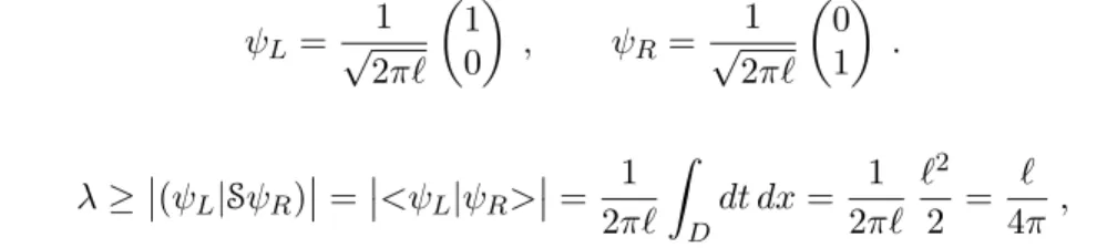
The traces of higher powers give additional geometric information, as is explained in the example of tr(S4) in Proposition 2.11. Then we explore the connection between the spectrum of S and the lengths of curves. We prove that length ℓ of any timelike curve is bounded from above by the largest eigenvalue λof Sby (Proposition 2.12)
λ≥ ℓ 4π .
Moreover, it is shown that the length ℓof any spacelike curve is bounded from above by the trace over the positive spectral subspace ofS (Proposition 2.13),
tr
χ(0,∞)(S)S
≥ ℓ 4π .
Finally, it is shown that the geometry of M is completely determined if S is given as an integral operator acting on the initial data set of any Cauchy hypersurface (Theorem 2.14).
In Section 3 we turn attention to themassivecase. A general solution of the Cauchy problem is constructed using the Green’s function which is given in terms of Bessel functions (Lemma 3.1). Next, we analyze how the regularity of the image of Sdepends on the smoothness of the boundary (see Propositions 3.3 and 3.4). This also makes it possible to estimate the asymptotics of the eigenvalues near the origin in terms of the total variation of the boundary curve (Theorem 3.7). In Proposition 3.12 it is shown that the spectrum of Sis again symmetric with respect to the origin, but with a different method than in the massless case. We proceed by computing the trace of powers of the fermionic signature operator. The dependence on the mass parameter gives additional geometric information, as is explained in Proposition 3.13 for the trace of S2.
1.3. Lorentzian Surfaces in the Massless Case. In generalization of the Minkowski drum, in this paper we also consider Lorentzian surfaces with curvature. The point of interest is to analyze how the curvature of the surface affects the spectrum of the fermionic signature operator. For technical simplicity, we restrict attention to the massless case. This case is mathematically appealing because we can make use of the conformal invariance of the massless Dirac equation, making the tools of conformal geometry available.
The structures introduced in Section 1.1 for the Minkowski drum all generalize to the setting with curvature: We let (M, g) be a two-dimensional globally hyperbolic Lorentzian manifold. Globally hyperbolic means that there is a space-like curve N being a Cauchy surface (for the precise definition of global hyperbolicity and a Cauchy surface see Section 4). The Cauchy surface can be either compact or non-compact.
In the first case, it is diffeomorphic to a sphere, whereas in the latter case, it is diffeomorphic to an open interval. For simplicity, we here restrict attention to the latter case. We let SM be the spinor bundle onM. The fibers SxM are isomorphic to C2. They are endowed with an inner product of signature (1,1), which we denote by ≺.|.≻x. The smooth sections of the spinor bundle are denoted by C∞(M, SM).
The Lorentzian metric induces a Levi-Civita connection and a spin connection, which we both denote by ∇. Every vector of the tangent space acts on the corresponding spinor space by Clifford multiplication. We denote the corresponding map from the tangent space to the linear operators on the spinor space by γ : TxM → L(SxM).
Clifford multiplication is related to the Lorentzian metric via the anti-commutation relations
γ(u)γ(v) +γ(v)γ(u) = 2g(u, v) 11Sx(M).
We also write Clifford multiplication in components with the Dirac matrices γj and use the short notation with the Feynman dagger, γ(u) ≡ujγj ≡u. The connections,/ inner products and Clifford multiplication satisfy Leibniz rules and compatibility con- ditions; we refer to [2, 29] for details. Combining the spin connection with Clifford multiplication gives the geometric Dirac operator D = iγj∇j. The massless Dirac equation reads
Dψ= 0.
We remark for clarity that in the case with curvature, the square of the Dirac operator no longer coincides with the wave operator. Indeed, by the Schr¨odinger-Lichnerowicz- Weitzenb¨ock formulaD2 =−∇j∇j+ R4 these operators differ by a multiple of scalar curvature R.
In the Cauchy problem, one seeks for a solution of the Dirac equation with initial data ψN prescribed on a given Cauchy surface N. Thus in the smooth setting,
Dψ= 0, ψ|N =ψN ∈C∞(N, SM).
This Cauchy problem has a unique solution ψ ∈ C∞(M, SM). This can be seen either by considering energy estimates for symmetric hyperbolic systems (see for ex- ample [27]) or alternatively by constructing the Green’s kernel (see for example [1]).
These methods also show that the Dirac equation is causal, meaning that the solution of the Cauchy problem only depends on the initial data in the causal past or future.
In particular, if ψN has compact support, the solution ψ will also have compact sup- port on any other Cauchy hypersurface. This leads us to consider solutions ψ in the classCsc∞(M, SM) of smooth sections with spatially compact support. On solutions in this class, one again introduces the scalar product (1.8), whereν/denotes Clifford mul- tiplication by the future-directed normal ν (we always adopt the convention that the inner product≺.|/ν.≻x is positivedefinite). Using current conservation∇j≺ψ|φ≻= 0, the scalar product (1.8) is independent of the choice of the Cauchy surface (similar as explained in Section 1.1 for the Minkowski drum). Now the fermionic signature operator Sis defined exactly as for the Minkowski drum by expressing the space-time inner product (1.9) in terms of the scalar product in the form (1.11).
For globally hyperbolic Lorentzian surfaces of finite lifetime and finite volume having a non-compact Cauchy surface, we show that the fermionic signature operator encodes the volume and the curvature in the following way. First, the Hilbert-Schmidt norm ofSagain encodes the volume (1.12), whereµnow is the volume measure corresponding to the Lorentzian metric. The formula for tr(S4) involves integrals of curvature:
tr S4
= 1 8π4
ˆ
M
dµ(ζ) ˆ
J(ζ)
exp 1
4 ˆ
D(ζ,ζ′)
R dµ
dµ(ζ′),
where J(ζ) denotes all space-time points which can be connected to ζ by a causal curve. Moreover, D(ζ, ζ′) is the causal diamond of the space-time pointsζ andζ′, i.e.
D(ζ, ζ′) = J∨(ζ)∩J∧(ζ′)
∪ J∨(ζ′)∩J∧(ζ)
, (1.13)
where J∨(ζ) and J∧(ζ) denotes the points which can be connected to ζ via a future- and past-directed causal curve, respectively.
Finally, we show that the geometry of M can be reconstructed if S is given as an integral operator acting on the initial data set of any Cauchy hypersurface (Theo- rem 4.11).
1.4. Outlook: The Chiral Index and Causal Fermion Systems. We now put the ideas and constructions given in this paper into a more general context, also indicating possible directions of future research.
We first point out that for simplicity, we here restrict attention to two-dimensional space-times and mainly the massless Dirac equation. But most constructions could be generalized to globally hyperbolic Lorentzian manifolds of arbitrary dimension.
The continuity of the space-time inner product (1.10) can be subsumed in the notion that the space-time should bem-finite, which means qualitatively that the space-time must have finite lifetime(for details see [20, Section 3.2]). However, many interesting space-times like asymptotically flat Lorentzian manifolds or Lorentzian manifolds with asymptotic ends have infinite life-time, implying that the continuity condition (1.10) fails. In such space-times, one must use a different construction which relies on the so-called mass oscillation property introduced in [19]. In all these situations, the con- nection between the spectrum of the fermionic signature operator and the geometry of the Lorentzian manifold is largely unknown, leaving many interesting mathematical questions open.
We next remark that it is possible to associate an index to the fermionic signature operator, which takes integer values. In [14] simple examples of space-times with a non-trivial index are constructed, and the stability of the index under homotopies is studied. But it is unknown if and how this index is related to the geometry or the topology of the space-time. In order to introduce this index, one needs as an additional structure a chiral grading operator Γ which acts on the spinor spaces and has for all u∈TxM the properties
Γ∗ =−Γ, Γ2 = 11, Γγ(u) =−γ(u) Γ, ∇Γ = 0, (1.14) whereγ is Clifford multiplication and the star denotes the adjoint with respect to the inner product ≺.|.≻x. More generally, the operator Γ is defined in any even space- time dimension by Clifford multiplication with the volume form. In physics, Γ is called
“pseudoscalar operator” and is usually denoted by γ5. The grading operator gives rise
to the two idempotent operators χL= 1
2 11−Γ
and χR= 1
2 11 + Γ ,
referred to as the chiral projections (on the left respectively right handed component of the spinors). The chiral signature operators SL and SRare defined by inserting the chiral projections into (1.11),
<φ|χL/Rψ>= (φ|SL/Rψ). The first relation in (1.14) implies thatS∗
L=SR. We thus define thechiral indexas the Noether index of SL (sometimes called Fredholm index; for basics see for example [30,
§27.1]),
indS:= dim kerSL−dim cokerSL
= dim kerSL−dim kerSR.
The fermionic signature operator is a technical tool in the fermionic projector ap- proach to quantum field theory and is also used for constructing examples of causal fermion systems. We now outline these connections. The fermionic projector P is ob- tained by composing the causal fundamental solution km with the projection operator on the negative spectral subspace of S,
P =−χ(−∞,0)(S)km. (1.15)
This distribution implements the physical concept of the “Dirac sea”. Next, particles and anti-particles are introduced to the system by adding to (1.15) additional occupied states or by creating “holes”. We refer the interested reader to the constructions in [20, Section 3] and the survey article [13].
It is a general idea behind the fermionic projector approach that the geometry of space-time as well as all the objects therein should be described purely in terms of the physical wave functions of the system. This idea is made mathematically precise in the notion of a causal fermion system as introduced in [16]. In order to get into this framework, one chooses Hparticle as a subspace of the solution space of the Dirac operator. A typical example is to choose Hparticle = χ(−∞,0)(S) as the image of the fermionic projector (1.15). By introducing an ultraviolet regularization, one arranges that the functions inHparticleare continuous (for details see [20, Section]). Then for any space-time point x, one can introduce the so-called local correlation operator F(x) ∈ L(Hparticle) via the relations
(ψ|F(x)φ) =−≺ψ(x)|φ(x)≻x for all ψ, φ∈Hparticle.
Denoting the signature of the spin scalar product by (n, n), the local correlation op- erator is a symmetric operator in L(Hparticle) of rank at most 2n, which has at most n positive and at most n negative eigenvalues. Finally, we introduce the universal measure dρ=F∗dµas the push-forward of the volume measure on Munder the map- pingF (thusρ(Ω) :=µ((F)−1(Ω))). Omitting the subscript “particle”, we thus obtain a causal fermion system as defined in [16, Section 1.2]:
Definition 1.1. Given a complex Hilbert space (H,h.|.iH) (the “particle space”) and a parameter n ∈N (the “spin dimension”), we let F ⊂L(H) be the set of all self-adjoint operators on H of finite rank, which (counting with multiplicities) have at most n positive and at most n negative eigenvalues. On F we are given a positive
M⊂R1,1 N
N D
(0,0) (0, b)
Figure 2. Choosing the Cauchy surface at t= 0.
measure ρ (defined on aσ-algebra of subsets of F), the so-called universal measure.
We refer to (H,F, ρ) as a causal fermion system.
Causal fermion systems provide a general mathematical framework in which there are many inherent analytic, geometric and topological structures. This concept makes it possible to generalize notions of differential geometry to the non-smooth setting.
From the physical point of view, it is a proposal for quantum geometry and an approach to quantum gravity. We refer the interested mathematical reader to the research papers [15, 17] or the introductory textbook [18]. In the setting of causal fermion systems, the physical equations are formulated in terms of the causal action principle (see [12]).
In the setting of causal fermion systems, the fermionic signature operator is simply defined by the integral
S=− ˆ
F
x dρ(x)
(this operator can be viewed as the restriction of the fermionic signature operator defined by (1.11) to Hparticle; for details see [14, Section 4]). In this context, the objectives of our “Lorentzian spectral geometry” generalize to the question of how the spectrum of S is related to the objects of the Lorentzian quantum geometry as introduced in [15].
2. The Massless Case
2.1. Simple Domains. Let M ⊂ R1,1 be an open, bounded, globally hyperbolic subset of the Minkowski plane R1,1 (see the left of Figure 2, where also one Cauchy surfaceN is shown). The maximal solution for initial values on a Cauchy surfaceN is defined on a causal diamond D in the Minkowski plane. The following constructions will depend only on the space of solutions in this causal diamond, but the choice of the Cauchy surface will be irrelevant. In particular, the Cauchy surface does not necessarily need to lie entirely in M. With this in mind, we simply choose N as the straight line joining the left and right corners of the causal diamond. Moreover, by a Poincar´e transformation we can arrange that the left corner is the origin, whereas the right corner has the coordinates (0, b) with a parameter b > 0. Then the scalar product (1.8) simplifies to
(ψ|φ) = 2π ˆ b
0 ≺ψ(0, x)|γ0φ(0, x)≻dx= 2π ˆ b
0 hψ(0, x), φ(0, x)iC2 dx (2.1) (where in the last step we used (1.7)).
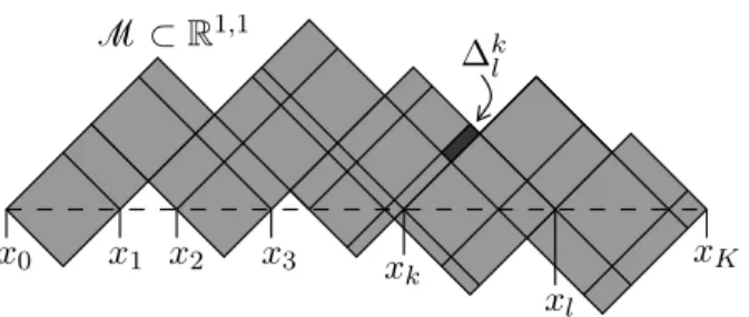
M⊂R1,1
x0 x1 x2 x3 xk xK
xl
∆kl
Figure 3. A simple domain.
For simplicity, we begin the analysis in the massless case. Then the Dirac equa- tion (1.4) has the general solution
ψ(t, x) =
ψL(t+x) ψR(t−x)
(2.2) with complex-valued functionsψLandψR. In view of (2.1), the left- and right-moving components are orthogonal. The following assumption makes it possible to analyze S explicitly.
Definition 2.1. M is a simple domain if there is a finite number of points 0 =x0 < x1<· · ·< xK =b
such that the boundary of M is contained in the lightlike curves through these points,
∂M⊂x0, . . . , xK +R(1,1) +R(1,−1).
The name “simple domain” is inspired by simple functions in measure theory which take only a finite number of values. Figure 3 shows an example.
We now introduce a basis ofH0 which will turn out to be an eigenvector basis ofS. To this end, for c∈ {L, R}, k∈ {1, . . . , K} and n∈Z we define functions which are plane waves on the subintervals,
ψck,n(x) = 1
p2π(xk−xk−1) χ(xk−1,xk](x)e
2πi xk−xk−1 nx
(2.3) (whereχdenotes the characteristic function). As in (2.2) we regard the functionsψRk,n andψLk,nas spinors in the first and second component, respectively. Solving the Cauchy problem, we obtain the corresponding Dirac solutions
ψLk,n(t+x) 0
and
0 ψk,nR (t−x)
,
which with a slight abuse of notation we again denote by ψk,nc ∈H0 (note that these are solutions only in the weak sense, as they are not continuous). A short computation shows that these vectors are orthonormal,
(ψck,n|ψkc′′,n′) =δc,c′δk,k′δn,n′. Using that the plane waves e
2πi xk−xk−1 nx
form a Fourier basis of L2((xk−1, xk]), one also sees that the vectors (ψk,nc ) form a basis of H0. Hence (ψck,n) is an orthonor- mal basis of H0. Moreover, a short computation shows that the space-time inner product <ψck,n|ψkc′′,n′>vanishes if nor n′ are non-zero (because one integrates over a
full period of a plane wave) or if c =c′ (because the inner product (1.7) involves an off-diagonal matrix). The remaining inner products are computed by
<ψRk,n|ψl,nL ′>=<ψLl,n′|ψRk,n>
= δ0nδ0n′ 2πp
(xk−xk−1)(xl−xl−1) µ(∆kl) = δn0 δn0′ 2π√
2 q
µ(∆kl), whereµ is the Lebesgue measure on R1,1 and
∆kl =
(xk−1, xk] +R(1,1)
∩
(xl−1, xl] +R(1,−1)
∩M (see Figure 3). We thus obtain the following result:
Lemma 2.2. On a simple domain M and for zero mass, the fermionic signature operator Shas finite rank. More precisely, choosing the orthonormal basis (2.3),
(ψck,n) with c∈ {L, R}, k∈ {1, . . . , K}, n∈Z,
it has rank at most 2K. It vanishes on all the vectors ψck,n with n 6= 0. On the subspace spanned by the basis vectors ψ1,0L , . . . , ψLK,0, ψR1,0, . . . , ψK,0R , it has the block matrix representation
S= 1 2π√
2
0 T∗
T 0
,
where T is the matrix with components Tlk=
q
µ(∆kl). (2.4)
From this matrix representation one can read off a few general properties of the spectrum of the fermionic signature operator:
Corollary 2.3. On a simple domain M and for zero mass, the following statements hold.
(i) The spectrum ofS is symmetric with respect to the origin and σ(S) =σ √
T∗T
∪ −σ √ T∗T
. For an eigenvectoruof √
T∗T corresponding to the non-zero eigenvalueλ, the eigenvectors of S corresponding to the eigenvalues±λ have the form
ψ= λu
±T u
.
(ii) The eigenvector corresponding to the largest eigenvalue ofSis non-degenerate.
Its components can be chosen to be non-negative.
(iii) Tr S2
= µ(M) 4π2 .
Proof. Follows from a direct computation. Part (ii) is a consequence of the Perron- Frobenius theorem for matrices with positive entries (see [38, Chapter 5]).
The spectrum of S does not determine the geometry completely, as the following example shows.
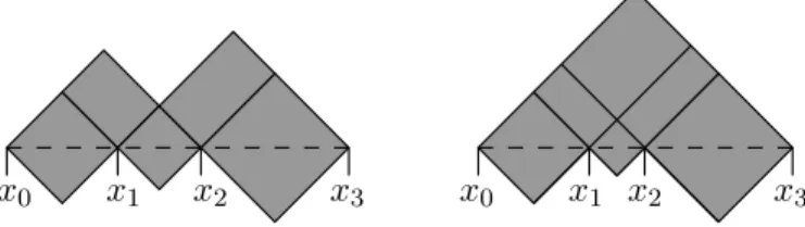
x0 x1 x2 x3 x0 x1 x2 x3
Figure 4. Simple domains corresponding to the matrices T (left) and ˜T (right).
Example 2.4. (Isospectral simple domains) Consider the matrices T =
a √
ab 0
0 b √
bc
0 0 c
and T˜=
d √
de √ df
0 e √
ef
0 0 f
,
wherea, . . . , f are strictly positive parameters. The form of the off-diagonal matrix el- ements ensures that these matrices can be realized in the form (2.4) by simple domains.
More precisely, in order to realize the matrix T, one choosesK = 3 and x1−x0=√
2a , x2−x1 =√
2b , x3−x2 =√ 2c .
The simple domain is then chosen as all the squares in the future, except for the square on top (see the Figure 4 on the left). The matrix ˜T is realized similarly by a simple domain with K = 3, but this time without removing the square on top (see Figure 4 on the right). Obviously, the resulting simple domains are not isometric. We want to show that for suitable values of the parameters, the matrices T∗T and ˜T∗T˜ are isospectral. In view of Corollary 2.3, this implies that the fermionic signature operators corresponding to the two simple domains are isospectral.
We choose the parameters d=e= 1 and f =δ with a small parameter δ > 0, so that
T˜=
1 1 √
δ
0 1 √
δ
0 0 δ
.
As a necessary condition for T∗T and ˜T∗T˜ to be isospectral, the matrices T and ˜T must have the same determinant (note that these determinants are obviously positive).
We satisfy this condition by choosing
c= δ ab.
Computing and comparing the characteristic polynomials of T∗T and ˜T∗T, one sees˜ that it remains to satisfy the conditions
−1 +a2b2−δ+aδ+bδ−3δ2+δ2 a2 +δ2
b2 + δ2
ab = 0 (2.5)
3−a2−ab−b2+ 2δ− δ
a+δ2− δ2
a2b2 = 0. (2.6) Multiplying the second equation by a2 and adding the first equation, we obtain a quadratic equation forbof positive discriminant. Choosing the explicit solution which forδ= 0 anda= 1 givesb= 1 (so that we get back the matrix ˜T), and substituting this
solution into (2.5), we obtain one equation for the remaining unknowna. Expanding this equation aroundδ = 0 and a= 1, we obtain the condition
5δ−8(a−1)2+O δ2
+O δ(a−1)
+O (a−1)3
= 0. Thus for sufficiently smallδ >0 there are solutionsaof the form
a= 1± r5δ
8 +O(δ).
We thus obtain a one-parameter family of isospectral pairs of matrices T∗T and ˜T∗T˜.
♦ 2.2. Representation ofS as an Integral Operator. LetM⊂R1,1 be a bounded, globally hyperbolic subset of the Minkowski plane. As explained at the beginning of Section 2.1, we again choose the Cauchy surface (0, b) at timet= 0.
Proposition 2.5. The fermionic signature operator can be represented as an integral operator
(Sψ)(x) = ˆ b
0
S(x, y)ψ(y)dy (2.7)
with a bounded integral kernel,
S(., .)∈L∞ (0, b)×(0, b),L(V)
. (2.8)
Proof. The Cauchy problem with initial data at t= 0 has the explicit solution ψ(t, x) =
ψL(0, x+t) ψR(0, x−t)
. (2.9)
Using this representation in (1.9), multiplying out and estimating each term gives
<ψ|φ>
≤ ˆ
M
kψR(0, x−t)k kφL(0, x+t)k+kψL(0, x+t)k kφR(0, x−t)k dt dx . Estimating the integral by the integral over the whole causal diamond, we obtain
ˆ
MkψR(0, x−t)k kφL(0, x+t)kdt dx
≤ ˆ
DkψR(0, x−t)k kφL(0, x+t)kdt dx
= 1 2
ˆ b
0 kψR(0, x)kdx ˆ b
0 kφL(0, x′)kdx′
. We conclude that for all ψ, φ∈H0,
<ψ|φ>
≤ ˆ b
0 kψ(0, x)kdx ˆ b
0 kφ(0, x′)kdx′
.
This means that the bilinear form <.|.> can be estimated in terms of theL1-norm of both arguments on the Cauchy surfacet= 0. In other words,
<.|.>∈L1 (0, b)×(0, b), dx dy∗ .
Since the dual space of L1(dx dy) is the Banach space ofL∞-functions acting by weak evaluation, we conclude that there is a kernel S(., .) ∈ L∞((0, b)×(0, b), dx dy) such that
<ψ|φ> = 2π ˆ b
0
ˆ b
0 hψ(x),S(x, y)φ(y)iC2 dx dy .
Comparing with (1.11) and (2.1) gives the result.
We remark that the estimates used in the proof of this proposition will be generalized and refined in Section 3.2.
The fact that the kernel is pointwise bounded (2.8) and the domain (0, b) has finite volume implies that the trace of any even power of S is finite and can be computed with the standard formula:
Corollary 2.6. The fermionic signature operatorSis Hilbert-Schmidt. Moreover, the traces of even powers of S2q, q∈N, are given by the integrals
tr(S2q) = ˆ b
0
dx1. . . ˆ b
0
dx2qTr S(x1, x2)· · ·S(x2q, x1)
, (2.10)
where trdenotes the trace of an operator on the Hilbert space, and Tr is the trace of a (2×2)-matrix.
Proof. According to (2.8), we know that kS(x, y)k ≤ C for almost all x, y ∈ (0, b) (where k · k denotes the Hilbert-Schmidt norm of a (2×2)-matrix). Hence
ˆ b 0
dx ˆ b
0
dy
S(x, y)
2 < C2b2. (2.11) We now choose on H0 = L2((0, b),C2) the orthonormal basis (ψcn) with n ∈ Z, c ∈ {L, R} given by plane waves
ψcn= 1
√2πbψc e2πib nx where ψL= 1
0
, ψR= 0
1
. Then Parseval’s identity for double Fourier series shows that the series
1 (2π)2
X
c,c′∈{L,R}
X
n,n′∈Z
(ψnc|Sψcn′′)
2
coincides with the integral in (2.11). We conclude that the operator S is Hilbert- Schmidt. Moreover, the trace of S2 can be computed by (2.10) specialized to the case q= 1.
By iterating (2.7) and using Fubini’s theorem, one obtains an integral representa- tion of the operator Sq again with a pointwise bounded kernel. Repeating the above argument with Sreplaced by the operatorSq, we conclude that also the operatorSq is Hilbert-Schmidt, and that its Hilbert-Schmidt norm can be computed by (2.10). This
concludes the proof.
This corollary shows in particular that the operator S is compact. Thus S has a pure point spectrum and finite-dimensional eigenspaces. Moreover, the eigenvalues can accumulate only at the origin.
2.3. Symmetry of the Spectrum. In Corollary 2.3 (i) we saw that for a simple domain, the spectrum is symmetric with respect to the origin. The next proposition shows why this is true even for general domains.
Proposition 2.7. The spectrum ofS is symmetric with respect to the origin.
Proof. The matrix
Γ :=
−1 0
0 1
(2.12) obviously anti-commutes with the Dirac matrices (1.6) and the Dirac operator (1.5), i.e. ΓD=−DΓ. Hence ifψ is a solution the massless Dirac equation, the same is true for Γψ. In other words, Γ maps the solution space of the Dirac equation to itself,
Γ : H0→H0.
Using (1.7), one sees that Γ is anti-symmetric with respect to the spin scalar prod- uct≺ψ|Γφ≻=−≺Γψ|φ≻. Moreover, using (1.8) and (1.9), we find that for all ψ, φ∈ H0,
<ψ|Γφ>= ˆ
M≺ψ|Γφ≻xdµ(x) =− ˆ
M≺Γψ|φ≻xdµ(x) =−<Γψ|φ> (2.13) (ψ|Γφ) = 2π
ˆ
N≺ψ|ν/Γφ≻xdµN(x) =−2π ˆ
N≺ψ|Γ/νφ≻xdµN(x)
= 2π ˆ
N≺Γψ|/νφ≻xdµN(x) = (Γψ|φ). (2.14) In view of (1.11), the eigenvalue equation Sψ=λψ can be written as
<φ|ψ>=λ(φ|ψ) for all φ∈H0.
Using the symmetries (2.13) and (2.14), one sees that if ψ is an eigenvector corre- sponding to the eigenvalue λ, then Γψ is an eigenvector corresponding to the eigen-
value−λ.
2.4. Computation of tr(S2q), Recovering the Volume. Proposition 2.5 also im- plies that the operatorsSpare trace class for anyp∈N. The symmetry of the spectrum shown Proposition 2.7 implies that the trace of an odd power of S vanishes. We now want to compute the trace of even powers of S. For computational purposes, it is most convenient to work with the causal fundamental solution in light cone coordi- nates. In order to keep the setting as simple as possible, we here introduce the causal fundamental solution k0 simply as a device for expressing the solution of the Cauchy problem.
Lemma 2.8. The solution ψ of the Cauchy problem
Dψ= 0, ψ|t=0 =ψ0∈C0((0, b)) has the representation
ψ(t, x) = 2π ˆ b
0
k(t, x−y)γ0ψ0(y)dy , (2.15) where k(t, x) is the distribution
k(t, x) = 1
4π (γ0+γ1)δ(t+x) + 1
4π(γ0−γ1)δ(t−x). (2.16) Proof. A direct computation using (1.6) shows that (2.15) indeed agrees with (2.9).
The distribution k(t, x) is referred to as the causal fundamental solution. At first sight, the method of this lemma seems unnecessarily complicated, because (2.9) is much simpler than (2.15). The advantage of (2.15) is that this formula generalizes to the massive case (see Section 3.1) and even to globally hyperbolic space-times in arbitrary dimension (see for example [20, Lemma 2.1]).
The integral in (2.15) can be regarded as atime evolution operator which maps the solution at some initial time t= 0 to the solution at a final time t. Clearly, if one first takes the time evolution from time t0 to t1 and then the time evolution fromt1 to t2, one gets the same as if one takes the time evolution directly from t0 tot2. This fact is often referred to as agroup propertyof the time evolution, where the group operation is the multiplication of the time evolution operators and the inverse of the time evolution from t0 to t1 is the time evolution from t1 to t0. This group property is reflected in a property of the causal fundamental solution. Namely, denoting a space-time point for simplicity by ζ = (t, x), we have for anyζ,ζ˜∈M,
k(ζ−ζ′) = 2π ˆ b
0
k(ζ0, ζ1−x)γ0k(−ζ˜0, x−ζ˜1)dx (2.17) (this relation can also be verified by direct computation using (2.16)). Moreover, one sees directly from (2.16) that the kernelk(t, x) is symmetric in the sense that
k(t, x)∗=k(−t,−x) (2.18)
(where the star denotes the adjoint with respect to the inner product ≺.|.≻x).
We next express the integral kernel ofSin terms of the causal fundamental solution.
Lemma 2.9. The kernel S(x, y) of the fermionic signature operator in (2.7) can be written as
S(x, y) = 2π ˆ
M
k(−t, x−z)k(t, z−y)γ0dt dz .
Proof. Using (2.15) in (1.9) and applying (2.18), we obtain
<ψ|φ>= 4π2 ˆ
M
dt dz ˆ b
0
dx ˆ b
0
dy≺k(t, z−x)γ0ψ(0, x)|k(t, z−y)γ0φ(0, y)≻
= 4π2 ˆ
M
dt dz ˆ b
0
dx ˆ b
0
dy≺ψ(0, x)|γ0k(−t, x−z)k(t, z−y)γ0φ(0, y)≻.
On the other hand, we know from (1.11) and (2.7) that
<ψ|φ>= ψ
ˆ b 0
S(x, y)φ(0, y)dy .
Comparing these formulas gives the result.
The light-cone coordinates (u, v) are defined by
u=t+x and v=t−x . (2.19)
Then du dv= 2dt dxand t= u+v
2 , x= u−v
2
∂u = 1
2(∂t+∂x) , ∂v = 1
2(∂t−∂x)
(to improve the readability we denote the indices u andv in roman style). Setting γu =γ0+γ1 and γv =γ0−γ1, (2.20) we obtain the anti-commutation relations
γu2
= 0 = γv2
,
γu, γv = 4. (2.21)
The Dirac operator (1.5) and the causal fundamental solution (2.16) become
D=iγu∂u+iγv∂v (2.22)
k(u, v) = 1 4π
γuδ(u) +γvδ(v)
. (2.23)
Combining Lemma 2.9 with the integral representation of Proposition 2.5, we can compute powers of the operator S. For example,
S2
(x, y) = ˆ b
0
S(x, z)S(z, y)dz
= 4π2 ˆ b
0
dz ˆ
M
d2ζ ˆ
M
d2ζ k˜ −ζ0, x−ζ1
k ζ0, ζ1−z γ0
×k −ζ˜0, z−ζ˜1
k ζ˜0,ζ˜1−y γ0. Now we can carry out the z-integral using the group property (2.17). This gives
S2
(x, y) = 2π ˆ
M
d2ζ ˆ
M
d2ζ k˜ −ζ0, x−ζ1
k ζ−ζ˜
k ζ˜0,ζ˜1−y γ0. Iterating this method, we obtain
Sp
(x, y) = 2π ˆ
M
d2ζ1· · · ˆ
M
d2ζp
×k −ζ10, x−ζ11
k ζ1−ζ2
· · ·k ζp−1−ζp
k ζp0, ζp1−y γ0. Taking the trace with the help of Corollary 2.6, one can again apply (3.2) to obtain
tr S2q
= ˆ
M
d2ζ1· · · ˆ
M
d2ζ2q Tr
k ζ1−ζ2
· · ·k ζ2q−1−ζ2q
k ζ2q−ζ1
. (2.24) This formula is generally covariant, showing in particular that the trace ofS2pis indeed independent of the choice of the Cauchy surface.
The above formulas can be simplified considerably using the form of the causal fundamental solution in light-cone coordinates (2.23) and (2.21). Namely,
k0 ζ1−ζ2
· · ·k0 ζp−1−ζp
k0 ζp−ζ1
= 1
(4π)pγuδ(u1−u2)γvδ(v2−v3)· · ·+ 1
(4π)pγvδ(v1−v2)γuδ(u3−u3)· · · . Taking the trace and again using (2.21), we get zero ifpis odd. Ifpis even, we obtain
Tr
k0 ζ1−ζ2
· · ·k0 ζp−1−ζp
k0 ζp−ζ1
= 1
(2π)p δ(u1−u2)δ(v2−v3) · · ·δ(up−1−up)δ(vp−v1)
+ 1
(2π)p δ(v1−v2)δ(u2−u3) · · ·δ(vp−1−vp)δ(up −u1).
(2.25)
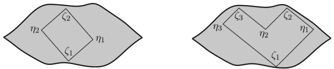
ζ1 η1 ζ2
η2
ζ1 η1 ζ2 η2 ζ3 η3
Figure 5. The geometric constraints given by Θ(ζ1, . . . , ζq) for q = 2 (left) andq = 3 (right).
Setting p = 2, we see that the result of Corollary 2.3 (iii) also holds for general domains:
Proposition 2.10. LetMbe a bounded, globally hyperbolic subset of Minkowski space.
Then the trace of S2 encodes the space-time volume, tr S2
= µ(M) 4π2 . Proof. Using (2.25) in (2.24) in the case p= 2, we obtain
tr S2
= ˆ
M
d2ζ1 ˆ
M
d2ζ2 2
(2π)2 δ(u1−u2)δ(v1−v2)
= 1
(2π)2 ˆ
M
d2ζ1 ˆ
M
d2ζ2 δ2(ζ1−ζ2) = µ(M) 4π2 ,
giving the result.
For general q, one can compute the trace of S2q with the following method. First, by renaming the variables one sees that the two summands in (2.25) give the same contribution to the trace. Thus
tr S2q
= 2
(2π)2q ˆ
M
d2ζ1 ˆ
M
d2η1· · · ˆ
M
d2ζq ˆ
M
d2ηq
×δ(u1−u˜1)δ(˜v1−v2) · · ·δ(uq−u˜q)δ(˜vq−v1),
(2.26) where the points ηj have the coordinates (˜uj,v˜j). Carrying out the integrals over η1, . . . , ηq, we obtain
tr S2q
= 2
(2π)2q 1 2q
ˆ
M
d2ζ1· · · ˆ
M
d2ζqΘ(ζ1, . . . , ζq),
where the function Θ(ζ1, . . . , ζq), which takes the values zero and one, gives geometric constraints for the position of the points ζ1, . . . , ζq. More precisely, introducing the points
η1= (ζ10, ζ21), η2 = (ζ20, ζ31), . . . ηq−1 = (ζq−10 , ζq1), ηq= (ζq0, ζ11), the function Θ is defined by
Θ(ζ1, . . . , ζq) =
1 ifη1, . . . , ηq ∈M 0 otherwise.
The geometric constraints are illustrated in Figure 5. Via these constraints, the trace of Sp depends on the geometry of the boundary curves ofM. While these constraints are rather complicated in general, in the case q = 2 they can be easily understood giving the following result.