Adiabatic Eliminations, and Local Searchers
Dissertation
zur Erlangung des akademischen Grades Doctor rerum naturalium
(Dr. rer. nat.) im Fach Physik
Spezialisierung: Theoretische Physik eingereicht an der
Mathematisch-Naturwissenschaftlichen Fakultät der Humboldt-Universität zu Berlin
von
Dipl. Phys., Jörg Nötel Präsidentin der Humboldt-Universität zu Berlin:
Prof. Dr.-Ing. Dr. Sabine Kunst
Dekan der Mathematisch-Naturwissenschaftlichen Fakultät:
Prof. Dr. Elmar Kulke
Gutachter:
1. L. Schimansky-Geier 2. H. Engel
3. E.E.N. Macau
Tag der mündlichen Prüfung: 04. 12. 2018
ABSTRACT
Active Brownian particles described by Langevin equations are used to model the behavior of simple biological organisms or artificial objects that are able to perform self propulsion. In this thesis we discuss active particles with constant speed. In the first part, we consider angular driving by whiteα-stable noise and we discuss the mean squared displacement and diffusion coefficients. We derive an overdamped description for those particles that is valid at time scales larger the relaxation time. In order to provide an experimentally accessible property that distinguishes between the considered noise types, we derive an analytical expression for the kurtosis. Afterwards, we consider an Ornstein-Uhlenbeck process driven by Cauchy noise in the angular dynamics of the particle. While, we find normal diffusion with the diffusion coefficient identical to the white noise case we observe a Non-Gaussian displacement at time scales that can be considerable larger than the relaxation time and the time scale provided by the Ornstein-Uhlenbeck process. In order to provide a limit for the time needed for the transition to a Gaussian displacement, we approximate the kurtosis.
Afterwards, we lay the foundation for a stochastic model for local search. Lo- cal search is concerned with the neighborhood of a given spot called home. We consider an active particle with constant speed and α-stable noise in the dy- namics of the direction of motion. The deterministic motion will be discussed before considering the noise to be present. An analytical result for the steady state spatial density will be given. We will find an optimal noise strength for the local search and only a weak dependence on the considered noise types.
Several extensions to the introduced model will then be considered. One ex- tension includes a distance dependent coupling towards the home and thus the model becomes more general. Another extension concerned with an erroneous understanding by the particle of the direction of the home leads to the result that the return probability to the home depends on the noise type. Finally we consider a group of searchers.
ZUSAMMENFASSUNG
Das Konzept von aktiven Brownschen Teilchen kann benutzt werden, um das Verhalten einfacher biologischer Organismen oder künstlicher Objekte, welche die Möglichkeit besitzen sich von selbst fortzubewegen zu beschreiben.
Als Bewegungsgleichungen für aktive Brownsche Teilchen kommen Langevin Glei-chungen zum Einsatz. In dieser Arbeit werden aktive Teilchen mit kon- stanter Geschwindigkeit diskutiert. Im ersten Teil der Arbeit wirkt auf die Bewegungsrichtung des Teilchen weißes α-stabiles Rauschen. Es werden die mittlere quadratische Verschiebung und der effektive Diffusionskoeffizient bes- timmt. Eine überdampfte Beschreibung, gültig für Zeiten groß gegenüber der Relaxationszeit wird hergleitet. Als experimentell zugängliche Meßgröße, welche als Unterscheidungsmerkmal für die unterschiedlichen Rauscharten herangezogen werden kann, wird die Kurtose berechnet. Neben weißem Rauschen wird noch der Fall eines Ornstein-Uhlenbeck Prozesses angetrieben von Cauchy verteiltem Rauschen diskutiert. Während eine normale Diffusion mit zu weißem Rauschen identischem Diffusionskoeffizienten bestimmt wird, kann die beobachtete Verteilung der Verschiebungen Nicht-Gaußförmig sein.
Die Zeit für den Übergang zur Gaußverteilung kann deutlich größer als die Zeitskale Relaxationszeit und die Zeitskale des Ornstein-Uhlenbeck Prozesses sein. Eine Grenze der benötigten Zeit wird durch eine Näherung der Kurtosis ermittelt.
Weiterhin werden die Grundlagen eines stochastischen Modells für lokale Suche gelegt. Lokale Suche ist die Suche in der näheren Umgebung eines bestimmten Punktes, welcher Haus genannt wird. Abermals diskutieren wir ein aktives Teilchen mit unveränderlichem Absolutbetrag der Geschwindigkeit und weißen α-stabilem Rauschen in der Bewegungsrichtungsdynamik. Die deterministis- che Bewegung des Teilchens wird analysiert bevor die Situation mit Rauschen betrachtet wird. Die stationäre Aufenthaltswahrscheinlichkeitsdichtefunktion wird bestimmt. Es wird eine optimale Rauschstärke für die lokale Suche, das heißt für das Auffinden eines neuen Ortes in kleinstmöglicher Zeit fest- gestellt. Die kleinstmögliche Zeit wird kaum von der Rauschart abhängen.
Wir werden jedoch feststellen, dass die Rauschart deutlichen Einfluß auf die Rückkehrwahrscheinlichkeit zum Haus hat, wenn die Richtung des zu Hauses fehlerbehaftet ist. Weiterhin wird das Model durch eine an das Haus ab- standsabhängige Kopplung erweitert werden. Zum Abschluß betrachten wir eine Gruppe von Suchern.
ACKNOWLEDGEMENT
First of all I would like to thank my supervisor Prof. Schimansky-Geier for discussions and critical remarks. I thank him for the scientific knowledge he shared and the anecdotes. I thank my second supervisor Prof. Macau for interesting ideas and his support especially during my stay in Brazil. I would also like to thank Prof. Sokolov as well as Bartek Dybiec for fruitful discussions.
David Hansmanns support on bureaucratic affairs and his personal engagement deserves special acknowledgment. João Eliakin, Frank Choque and Vander Freitas made me feel welcome during my stay in Brazil. I thank Christophe Haynes, Fabian Baumann, Malte Kähne, Patrick Pöschke and Justus Kromer for helpful discussions and their support. This work was supported through the DFG by the IRTG 1740.
SELBSTSTÄNDIGKEITSERKLÄRUNG
Ich erkläre, dass ich die Dissertation selbstständig und nur unter Verwendung der von mir gemäß §7 Abs. 3 der Promotionsordnung der Mathematisch- Naturwissen-schaftlichen Fakultät, veröffentlicht im Amtlichen Mitteilungs- blatt der Humboldt-Universität zu Berlin Nr. 126/2014 am 18.11.2014 angegebe- nen Hilfsmittel angefertigt habe.
Jörg Nötel Ort, Datum
PREFACE
Parts of the material in this thesis have been previously published, or submitted for publication. Most results of section II A were published in [1],[2] and [3].
The majority of the results of section II B were published in [1]. Main parts of section III have been submitted for publication [4] and [5].
CONTENTS
Selbstständigkeitserklärung vii
Preface ix
I. Introduction 1
A. Brownian Motion 4
B. Active Brownian Particles 6
1. Active Brownian Motion 6
2. The Limit Of Constant Speed 8
C. Stable Distributions 9
D. The Fokker Planck Equation 12
E. Adiabatic Elimination For Brownian Particles 13 II. Active Brownian Particle With Constant Speed And Angular Driving 16
A. Active Brownian Particle With Angular Driving By Whiteα-Stable
Noise 16
1. Mean Squared Displacement And Diffusion Coefficient 18
2. Coarse Grained Description 20
3. Kurtosis 28
B. Active Brownian Particle With Angular Driving By An
Ornstein-Uhlenbeck Process For The Cauchy Distribution 33 1. Mean Squared Displacement And Diffusion Coefficient 34
2. Displacement Distribution 35
3. Kurtosis 38
C. Discussion 41
III. A Model For Local Search 43
A. The Model 44
B. The Deterministic Model 47
1. Fixed Points And Separatrices 48
2. The Oscillatory (r, z) Dynamics 48
3. Period Length And Shift Of The Position Angle 50
4. Dynamics In The (x, y)Plane 51
5. Newtonian Mechanics 52
C. The Stochastic Model 53
1. Stochastic Dynamics 54
2. Spatial Distribution 55
3. The Relaxation Time τ 57
D. Local Search 62
1. Sojourn Time 62
2. Mean First Hitting Time 64
E. Reset At The Home 66
F. Distance Dependent Coupling 68
G. Limited Knowledge Of The Position Angle 71
1. The Deterministic Case 72
2. Stochastic Dynamics 73
H. Groups Of Searchers 80
I. Discussion 86
IV. Conclusion 89
A. Appendix 91
1. Moments Of The Angular Dynamics 91
2. Higher Moments Of The Velocities 92
3. Telegraphers Equation 92
4. Kurtosis OUP Cauchy 93
5. Derivation Of The StochasticX-Dynamics 94
6. Derivation Of The Overdamped Smoluchowski-Equation 95
References 97
LIST OF ABBREVIATIONS AND SYMBOLS Abbreviations
• ABP - active Brownian particle
• CLT - central limit theorem
• EQM - equation / equations of motion
• FPE - Fokker Planck equation
• l.h.s. - left hand side
• MSD - mean squared displacement
• OUP - Ornstein Uhlenbeck process
• PDF - probability density function
• r.h.s. - right hand side
• RTP - run and tumble particle
• SDE - stochastic differential equation Symbols
• ⟨...⟩- ensemble averaged property
• ⟨...⟩ϕ - ensemble average over ϕ
• δ(...) - Dirac delta distribution
• δij - Kronecker delta
• ξ(t)- noise, or random fluctuating force
• x˙ - total time derivative of x
• ⃗ev - unit vector in direction of v
• Θ(x) - Heavyside stepfunction with Θ(x) = 0 for x < 0 and Θ(x) = 1 otherwise
I. INTRODUCTION
The motion of living organisms has received much interest over the past years [6]. Modern tracking techniques and other elaborated tools allowed for exper- iments that lead to the description of observed trajectories, examples are the works on dicstyostelium [7], also under influence of chemotactic stimulus [8], on human motile keratinocytes and fibroblasts [9], on motile pieces of physarum [10], on flagellate eukaryotes (euglena) [11], also in time dependent light fields [12], and on more complex organisms as gastropods [13], zooplankton [14, 15], birds [16] and zebra-tail fish [17]. The presence of boundaries has been consid- ered [18, 19]. Also non-living motile objects, so called self-propelled particles, have been studied [20–23].
Observed trajectories are often stochastic. They are almost deterministic at certain short time scales and at diffusive larger times. As the particles are diffusive at large time scales, they remind of Brownian motion and therefore of thermal equilibrium. Hence to apply measures from statistical physics seems reasonable, but self-propelled particles, or living organisms with a propul- sion mechanism are systems out of thermal equilibrium. So, the physics out of equilibrium can be researched with seemingly simple objects. Therefore, velocity distributions [7–11] have been investigated and described. The dis- tribution of the directions in which the particles move has been considered [8, 11, 12, 14, 15, 17, 21]. The important properties of random motion like the mean squared displacement (MSD) and the diffusion coefficient have been studied [10, 14, 17, 18, 20, 21, 24]. The displacement distribution, a prop- erty that requires an even better statistics, has been measured [13, 22]. The escape over a barrier, or from a potential of self-propelled particles has been discussed [25, 26]. All those investigated properties might differ if a propulsion mechanism for a particle is present, or absent.
One aspect of studying individual trajectories can be an optimal foraging strat- egy [13, 15, 16, 27].
Individual motion can lead to the emergence of collective behavior, such as col- lective motion [28–30] or pattern formation [31–34] and alternating dynamics [35], while the underlying interactions are still investigated [36–39]. Outgoing from individual descriptions of the motion the information transfer [40, 41]
and decision making within a group has been investigated [42–44].
To model such motile units different models have been employed [45–47], like run and tumble motion [48–50], where particles follow a rather straight path and suddenly change direction or the model employed in [42], or random walks [51], or so called active Brownian particles (ABP).
In this work we will be concerned with the ABP. The ABP will be formally introduced in section I B. The word “Brownian” in ABP reminds of the stochas- tic nature of the trajectories of the particle and the word “active” refers to a propulsion mechanism that allows the particle to move without external forces [31]. Concepts considering an intake of external energy and converting it to motion have been discussed in [46, 52]. Due to the intake and transformation of energy into motion such particles represent systems far from thermodynamic equilibrium. We describe such a particle by means of the Langevin equation [53].
In this work, we will consider particles with constant speed. Constant speed can be a good approximation of experimental findings [17, 51] and is concerned in theoretical literature [54–58]. Existing theoretical work will be extended to angular driving with α-stable white noise sources and the special case of an Ornstein-Uhlenbeck process driven by white Cauchy distributed noise. The chosen cases allow for analytical treatment and are of relevance to experimen- tal observations as different turning angle distributions [15, 51] are observed in experiments. Different turning angle distributions result from different noise sources in the considered model. Turning angle distributions have been con- sidered to be related to foraging strategies [15].
We focus on stochastic properties. We introduce stable distributions and α- stable white noise in section I C and discuss the corresponding Fokker-Planck equation, which is a partial differential equation for the probability densities for systems described by Langevin equations, in section I D. The numerical method employed for simulations is also briefly elaborated in I C.
In chapter II we discuss particles with angular driving subjected to a constant torque as well as α-stable white noise. We will discuss the mean squared displacement (MSD) of the active particles, as well as the diffusion coefficient in dependence of the noise type given by the corresponding stable distribu- tions. We determine the relaxation time and show that in all those considered cases the active particles perform normal diffusion for times larger than the relaxation time. By means of an adiabatic elimination, we will derive a coarse grained description in section II A 2 for the active particles with constant speed, constant torque and α-stable noise acting on the direction of motion.
We will discuss that this coarse grained description is valid for times larger than the relaxation time and at length scales larger than the speed multiplied by the relaxation time. For the derivation of the coarse grained description, we first consider Gaussian white noise and discuss the procedure on the basis of the Langevin equation and afterwards discuss the elimination for the general α-stable noise on the basis of the FPE. We will derive the long term marginal probability density for the displacement. It will be Gaussian. It will turn out that neither the MSD nor the coarse grained description are suitable for distinguishing the noise type from experimental measurements of the MSD, we therefore analytically derive the kurtosis for the given system with vanish- ing torque in section II A 3. The kurtosis allows the distinction between the different α-stable noise types.
As second part of chapter II B, we consider a colored noise source for the pre- vious model, namely an Ornstein-Uhlenbeck process driven by white Cauchy distributed noise. The motion of particles with this particular colored noise display a run and tumble behavior. This choice for the noise allows for an exact calculation of the MSD and the diffusion coefficient. We will show, that particles subjected to this particular noise source perform normal diffusion.
Surprisingly, due to the specific properties of the colored noise source the re- sulting MSD is equal to a particle with angular driving by white Cauchy noise but the transition to the Gaussian displacement will happen on a different time scale. Through an approximation of the kurtosis we will provide a time scale for the transition to the Gaussian displacement.
We will discuss the findings of chapter II in II C.
In chapter III we will lay the foundation for a stochastic model for local search [59]. Local search is concerned with the neighborhood of a given spot called home. The particle explores the vicinity of the home and repeatedly returns towards it. Local search is known to be performed by insects such as flies and ants [51, 60–63] and is considered to fulfill the purpose of foraging.
The use of noise in global search problems is very popular [64]. For non-local search the use of Lévy Flights and of α-stable white noise have proven to be effective [16, 27]. The consideration of noise in models of local search is rare.
The use of power law distributed step lengths to explore the neighborhood of a certain spot seems to be counterproductive.
The local search is observed for objects which are able to keep track of distances and orientations as they move and use these information to calculate their current position in relation to a fixed location. If the position of the home and the angle towards the home are known then the method is called path integration [27, 59, 65, 66] and the specific exploration behavior might be based on some internal storage mechanism [67, 68] or external cues [69] as for example special points of interest or pheromonic traces, etc.
In our stochastic model we orientate ourselves on studies and experiments concerned with ants, bees and flies [51, 62, 63]. For these insects local search is observed. Especially, the various two dimensional spatial patterns which the local searchers draw during their motion have received a lot of interest [60–62, 70–72]. A profound mathematical explanation based on principles of stochastic dynamics seems to be still a challenge.
A better understanding of local search problems is also of technical interest.
Spatial exploration performed by robots [73] are planned for the ocean [74–77]
and space [73, 77]. Autonomous vehicles [76, 78] might move inside an area, around a chosen point, sometimes visit it and return to the local search using internal cues instead of external ones [79, 80].
In section III A we introduce the model. Our model does not distinguish between search and return. Both features follow the same law. The introduced model is similar to the deterministic Mittelstaedt bicomponent model [70–72].
However our model contains a noise source and we can generalize the model to a class of models by considering different distance dependent couplings in section III F. We will thoroughly discuss the deterministic system and its properties in section III B, before we consider the noise to be present in section III C 1.
We consider different turning behavior throughα-stable noise. We will discuss the steady state spatial density of the particles. Surprisingly, the steady state spatial density will not depend on the noise strength and also not depend on the noise type.
As local search is often considered to be foraging, we will investigate the av- erage time for discovering a new food source. We will find an optimal noise strength for a minimal average time (mean first hitting time) of discovering a new food source. This optimal noise strength will be for all considered noise types roughly equal. The minimal average time will not significantly depend on the noise type. We will explain this optimal noise strength by two counter- acting effects of the noise.
As the searcher repeatedly returns to the home, we consider in III E a more
realistic scenario for the mean first hitting time of a new food source, where the searcher, when it has returned to the home, chooses a new random outgoing direction. Simulation results will show that the optimal noise strength for minimal search time still exists, but is shifted to smaller values due to this additional random effect.
In section III F we extend the studied model to a distance dependent coupling.
For such distance dependent coupling a variety of functions that can be ex- pressed by a power series can be considered. We derive the steady state spatial density and other stochastic properties and we argue that an optimal noise for minimal search time for this class of models exist.
While for the model so far the active particle always needs to know exactly its position angle, we investigate in III G in the most simple way the consequences of an erroneous understanding of this position angle. We will find approxima- tions for the steady state spatial density in the small noise strength limit and in the large noise strength limit. The noise type and strength in the model relate to turning angles. Those results seem to indicate that a specific turning behavior might not be related to optimization of the search time but instead that the specific turning behavior of the searcher is related to the probability to return to the home, if an erroneous understanding of the position angle is present. An erroneous understanding of the position angle might arise as the active particle constantly internally needs to update/redetermine this position angle.
Finally, we will discuss the findings of chapter III in III I.
While we have used already several times the terms active Brownian parti- cle (ABP) and α-stable noise, we will formally introduce these terms in the following sections of this introduction.
A. Brownian Motion
Before considering the “active” part of ABP, we will discuss the “Brownian”
part. The term Brownian reminds of the stochastic nature of the motion, reminds of the seemingly random influences, in many cases complex or un- traceable forces acting on the motion, that we call noise. Brown studied the random motion of pollen of plants in a fluid under a microscope [81]. As we understand now, through the works of Einstein [82, 83], Smoluchowski [84]
and Langevin [53] the random motion is caused by the interaction of the fluid molecules with the pollen. Einstein derived results for the overdamped regime, neglecting inertia. Langevin [53] started from a Newtonian equation of motion and took therefore inertia into account. He introduced a random force ξ(t) acting on an observed particle at positionx, with velocity v
˙ x=v
mv=˙ −γv+√
2γkBT ξ(t). (I.1)
The mass of the particle is given by m, the Stokes friction coefficient is γ and kBT is the thermal energy, withkBbeing the Boltzmann constant andT being the absolute temperature. The first term on the r.h.s. is called: deterministic drift. Langevin assumed the random forcesξ(t)to be symmetric around zero, independent of position x and velocity v and also short correlated in time
t. The square root in front of the random forces is its strength. Langevin further assumed m⟨v2⟩ = kBT following the Maxwellian velocity distribution in thermal equlibrium and the equipartition theorem. Ornstein and Uhlenbeck [85] considered the random force or noise to have zero mean ⟨ξ(t)⟩ = 0. The correlation at two instances in time t1 and t2 was supposed to exist only for very small differences |t1 −t2|. Here, we assume aδ-correlation⟨ξ(t1)ξ(t2)⟩= δ(t1−t2). The noise ξ(t) is Gaussian distributed. The process given by (I.1) is called Ornstein-Uhlenbeck process [85].
An equation like the second equation in (I.1) is called Langevin equation, or stochastic differential equation (SDE).
Given the property of the mean of the noise, we can average (I.1) over the noise realizations and derive the mean velocity [53, 85]
⟨v(t)⟩=v0exp(
−γ mt)
(I.2) with v0 = v(t = 0) being the initial condition. The mean velocity decays exponentially due to the friction and vanishes in the long time limit t ≫ τγ, with
τγ =m/γ . (I.3)
The mean displacement
⟨x(t)⟩= v0m γ
[1−exp(
−γ mt)]
, (I.4)
with initial position x(t = 0) = 0, is the distance traveled with the mean velocity. If the initial velocity vanishes v0 = 0, either because the observed particle has no velocity at the beginning of the experiment, or by taking an average over an ensemble of particles immersed in a resting fluid in thermal equilibrium, then the mean values for the velocity, and the displacement vanish, as the random fluctuating forces act in positive and negative direction equally.
The second moment of the velocity was calculated in [85]
⟨v2(t)⟩= kBT
m +
(
v20− kBT m
) exp(
−2γ mt)
(I.5) and shows an exponential decay towards the equipartition value. With absent initial velocity v0 the kinetic energy of the particle
⟨E⟩= kBT
2 − kBT 2 exp(
−2γ mt)
(I.6) increases with time till the equipartition value is reached for t ≫ τγ. Energy is pumped into the particle through the fluctuating forces. With large enough initial velocity v0 >√
kBT /m energy is drawn from the particle.
The mean squared displacement and the diffusion coefficient are two impor- tant experimentally accessible properties of random motion and where already measured in 1913 for ciliate [24]. Integration of (I.1) leads to the mean squared displacement (MSD)
⟨x2(t)⟩= 2kBT γ
[ t+ m
γ (
exp (
−m γ t
)
−1 )]
, (I.7)
with the initial conditions x(t = 0) = 0, v(t = 0) = v0 = 0 as was shown by [53, 85]. In the limit t ≪ τγ the motion is ballistic, while for t ≫ τγ the motion is normal diffusive. The time scale τγ corresponds to a length scale lγ = τγ
√kBT /m, called the brake path [86, 87]. At length scales smaller than the brake path the motion is ballistic, while at larger ones diffusive. The diffusion coefficient reads [53]
D= 1
2t⟨x2(t)⟩= kBT
γ , (I.8)
which is the result of Einstein [82], that related mobility µ = 1/γ with the diffusion coefficient and it is a fluctuation dissipation theorem.
Concluding this section, we say: the Brownian part in ABP refers to stochastic motion, expressed through a Langevin equation. We will discuss later, the MSD, the diffusion coefficient and the overdamped limit for the models in chapter II.
B. Active Brownian Particles 1. Active Brownian Motion
According to the review [46] the term “Active Brownian Particles” was in- troduced into physics in the year 1995 in [31]. There, the ABP referred to diffusing particles with the ability to generate a self-consistent field that in turn influences the motion of the particles [31]. The ABP was introduced in order to study structure formation. Later on, the emphasis was also put on active motion, considering particles that are able to perform individual motion out of gaining and storing kinetic energy from the environment [52] to model animal mobility. The term “active” can be generally associated with the ability to transform available energy into systematic motion [45].
A generic expression for the dynamics of a set ofN ABPs [31, 46] can be given by a set of Langevin equations, like
⃗r˙i =⃗vi (I.9)
and
mi⃗v˙i =−γi(⃗ri, ⃗vi)⃗vi+f⃗i(r,v, t) +σiξ⃗i(t) (I.10) where the indexi= 1, .., N represents a particle number,mithe particles mass, xi its position in space, vi the corresponding velocity. The coefficient γi(⃗ri, ⃗vi) is now not only a friction coefficient but also expresses the active motion, mean- ing it ensures a finite non vanishing average velocity. Examples for a choice of active friction would be the Schienbein-Gruler model, see [88] and references therein, withγi(⃗ri, ⃗vi)⃗vi =γ⃗vi−γv0⃗vi/|⃗vi|, or the Rayleigh-Helmholtz friction, see [46] and references therein, with γi(⃗ri, ⃗vi)⃗vi =γ⃗vi2⃗vi−γv02⃗vi. In both ex- amplesv0 >0stands for a constant speed andγ >0for a constant coefficient.
If the velocity is smaller than the speed |⃗v| < v0 the friction term is negative and the particle gains speed. If the velocity is larger than the speed |⃗v| > v0
the friction is positive and the particle loses speed. The first term in both
examples for active friction terms is a dissipative force and causes a loss of mo- mentum, while the second term causes the gain of it. The Schienbein-Gruler approach reduces for vanishing v0 and with vanishing interaction term fi in the Langevin equation to normal Brownian motion. The functionfi stands for possible interactions between the particle i and the surrounding given by the tuple r = (⃗r0, ⃗r1, ..., ⃗ri, ..., ⃗rN), v = (⃗v0, ⃗v1, ..., ⃗vi, ..., ⃗vN). The kinetic energy
⟨Ei⟩ averaged over the noise of a non interacting particle fi = 0, with the given Langevin equation (I.10) can be expressed by
⟨E˙i⟩=⃗v⃗v˙ =−γi(⃗ri, ⃗vi)⃗vi2
. (I.11)
Hence, for negativeγi <0, the particle gains energy, energy is pumped into the system, while for positive active friction γi >0 the particle loses energy [46].
This way a Brownian particle can become an active Brownian particle. The system described by such equations (I.10) becomes out of thermal equilibrium.
The Einstein relation is invalid.
The function fi(x,v, t) stands for possible interactions with the environment and/or other particles. The symbols x and v stand for n-tuple containing the positions ⃗rj and velocities ⃗vj of all particles. We have not specified the noise yet. For now, we assume the noiseξ⃗i(t) = (ξx,i(t), ξy,i(t))to be Gaussian white noise, independent for each direction (x, y) and with ⟨ξi(t)⟩ = 0 and
⟨ξm,i(t1)ξn,j(t2)⟩ = 2δmnδijδ(t1 −t2), with m, n ∈ [x, y]. We chose the factor 2 to be consistent with the notation in the following chapters, an explanation for this particular parametrization follows in section I C. The parameter σi is the noise strength. If the noise strength σi is a constant as indicated, we call the noise ”additive“, otherwise the noise will be called ”multiplicative”.
The noise appearing in this thesis will be mostly additive, but multiplicative noise appears at some points, for instance in sections II A 2 a and III C. There the multiplicative noise, will appear in the form
˙
x=σ(x)ξ(t), (I.12)
with x being a scalar variable. When dealing with multiplicative noise the matter of interpretation arises. An illustrative introduction into multiplicative noise is given in [89]. There, the noise ξ(t) in equation (I.12) is considered to be white shot noise, meaning
ξ(t) =∑
i
δ(t−ti) (I.13)
that at instances of time ti the noise will cause a jump of x. The amplitude of the jump is proportional to σ(x) and then in [89] the question is raised, what is the correct x-value to take for the amplitude: after, before, in the middle the jump? A long story short: It is not a priori defined, one has to interpret.
If one takes the x value at the beginning of the jump, one interprets the SDE (I.12) in the Ito sense, if one takes the average value of the end position and the beginning the interpretation is called Stratonovich [90]. An SDE interpreted in the Stratonovich sense, can be transformed into a SDE which is then to be interpreted as Ito, and vice versa. In the given example (I.12) the Stratonovich interpretation is physically reasonable [89]. If a Langevin
equation is interpreted in the Stratonovich sense normal rules of calculus can be applied and in the given example (I.12) it is possible to divide by σ(x) and therefore transform the equation into an equation with additive noise [89].
Aside from Ito and Stratonovich, other interpretations are possible and depend on the physical situations [91]. We will point out the chosen interpretation at the respective situations.
2. The Limit Of Constant Speed
An often found approximation is considering self propelled particles in the limit of constant speed [54–58]. It can be a good approximation of experimental findings [17, 51]. Following [46] we derive here Langevin equations for an ABP with constant speed. Considering Langevin equations for a single, non interacting particle with massm = 1 and the Schienbein-Gruler friction
⃗r=˙ ⃗v =v⃗eh
⃗v=˙ −γ(v−v0)⃗eh+σhξh(t)⃗ev+σϕξϕ(t)⃗eϕ (I.14) the dynamics of the speed v = |⃗v| and the angular dynamics ϕ are written here such that they can be expressed separately, as is elaborated in [46]. The friction coefficientγ >0and the speedv0 >0of the Schienbein Gruler friction term are constants, the unit vector
⃗ev = ⃗v h =
(cosϕ(t) sinϕ(t)
)
(I.15) points in the direction of the heading of the particle and the unit vector
⃗eϕ=
(−sinϕ(t) cosϕ(t)
)
(I.16) is orthonormal to⃗eh. Here, we implicitly introduced another concept of ABP’s - the heading. Thinking of one possible realization of active particles as living motile objects, we have to consider head and tail. So, our particle has a head, hence a heading direction and a tail. For negative speed, the particle is assumed to move backwards.
The noise termsξv(t)and ξϕ(t)are independent from each other and act inde- pendently on the speed and the heading direction. They are Gaussian white noises with ⟨ξi⟩ = 0 and ⟨ξi(t1)ξj(t2)⟩ = 2δijδ(t1 −t2) and i, j being v or ϕ and with different noise strength σi. For the choice of the factor of 2 for the variance of the noise, we refer to section I C The way the noise acts on the velocities in equation (I.14) is different from the way it acts in the generic example (I.10). In the generic example the noise acted in the directions given by the Cartesian frame of reference, like something external, here the noise acts in the heading direction and orthogonal to it, like engine fluctuations and fluctuations in the choice of the heading. We call this first type passive noise and the second active noise [46]. The mechanisms acting behind active noise in propulsion direction might be internal engine fluctuations, or external rea- sons that can cause a slowing down and speeding up, like moving through a crowd and the fluctuations in the heading direction might be related to the
distribution of food, or internal mechanisms like ”thinking“. Active noise can cause a non Maxwellian velocity distribution even for a quasi Brownian par- ticle (v0 = 0) [46]. The active noise causes a pronounced peak at v = 0 in the velocity distribution, while passive noise leads to the thermal equilibrium distribution, the Maxwell distribution [46]. The noise as given in (I.14) is mul- tiplicative, so we interpret the equation in the Stratonovich sense [90], which allows for the normal rules of calculus to be applied.
While equation (I.14) is written in Cartesian coordinates, a description in the coordinates (v, ϕ)by two decoupled stochastic differential equations was given in [46]:
˙
v=γ(v0−v) +σhξh(t)
vϕ=˙ σϕξϕ(t), (I.17)
one for the absolute value of the velocity v and one for the heading direction ϕ. For large friction coefficient γ → ∞ the limit of constant speed is reached (v =v0) and the dynamics of the active particle reduces to
⃗r=˙ v0
(cosϕ(t) sinϕ(t) )
ϕ=˙ σϕ
v0
ξϕ(t), (I.18)
which was shown in [46].
Note, that the noise in the separated limit is additive (I.18). The appearance of the speed v0 in the angular dynamics is worth pointing out. It follows naturally in the derivation and reflects that it is more difficult to change the direction of motion at higher speed.
The models of active particles considered in this thesis are particles with con- stant speed and active fluctuations on the angular dynamics. We consider a class of noise sources called α−stable distributions.
C. Stable Distributions
Gaussian white noise is the most common noise source used in stochastic differ- ential equations, for instance it approximates the influence of a heat bath very well [53, 85]. Gaussian white noise is associated with thermal noise. There are not only physical reasons why it is often used, another reason is more mathematical, it states that the sum of independent and identical distributed random numbers with finite variance always converges to a Gaussian distribu- tion. This is one result of the central limit theorem (CLT). Noise in dynamical systems is often justified as a sum of random, often not tractable forces, or influences. So, the use of Gaussian white noise is founded on approximations of experimental observations as well as mathematical reasoning.
However, in the field of active Brownian particles it must not be the first choice.
Let’s assume for a moment a mosquito, or a fly moving, for simplicity, with constant speed and Gaussian white noise driving the angular dynamics, as given in the previous section (I.18). Gaussian white noise means a continuous diffusive motion of the angular variable ϕ. How easy would it be to catch the mosquito! Hence, the investigation of different noise sources and therefore of
different random turning behavior is reasonable and the life of a mosquito de- pends on it. Experimental evidence for Non-Gaussian noise sources appearing in the description of the motion of animals are discussed in [15, 16, 51, 92].
We will employ α− stable noise in the considered models. Random variables are called strictly stable, if for independent random variablesX1 and X2 being elements of the same distribution the linear combination
c1X1+c2X2
=d cX , (I.19)
with c, c1, c2 being constants holds [93]. The symbol =d refers to equality in distribution, meaningX belongs again to the same distribution asX1 andX2. The corresponding distribution is called strictly stable. It can be shown that the constantchas to fulfill the conditioncα =cα1+cα2 [93], withα ∈(0,2], hence the word α−stable with the stability index α. There is a distinction between strictly stable and stable, as stable allows for an additional constant on the r.h.s of (I.19). We will always consider strictly stable distributions, although we write only stable. We will always consider distributions symmetric to zero, X =d −X, - symmetric α−stable noise. Equation (I.19) means that the shape of a distribution is stable [93].
Stable distributions are of special interest as the central limit theorem states that the sum of independently and identically distributed random variables converges to a stable distribution [93]. If the variance of the variables is finite the stable distribution will be Gaussian.
The probability densityP(X)for the random variableXcan be best expressed by its Fourier-transform, or characteristic function
ϕ(k) =
∫ ∞
−∞
dXexp (ikX)P(X) . (I.20) The characteristic function of a symmetric α−stable distribution, with scale parameterσ has the form:
ϕ(k) = exp (−σα|k|α) , (I.21) with α ∈ (0,2]. The scale parameter is what we called previously noise strength. Further on we will usually call it noise strength, except in this math- ematical subsection. Closed form expressions for the densities of symmetric stable distributionsP(X)are known forα= 2, the Gaussian distribution, and α = 1, the Cauchy distribution, while for other values of α only expressions as a series exist [94]. Note, that the scale parameter σ is not equal to the standard deviation of the corresponding Gaussian density(α = 2). The stan- dard deviation would be√
2σ. Because of the convention for the characteristic function, we chose in the previous section I B for the correlation the factor of 2,⟨ξ(t1)ξ(t2)⟩= 2δ(t1−t2).
Figure 1 displays the probability density functions (PDF) P(X) of random variables X of symmetric stable distributions for various α. The blue solid line is the Gaussian density α = 2. When decreasing α, the peak of the density becomes more pronounced and the tails become heavier. The asymp- totic behavior X → ∞ of the PDF of a symmetric stable distribution is P(X)∼ασαX−(α+1) [93]. Those are the so-called power law tails.
-5 0 5 0
0.2 0.4 0.6
0.8 = 2.0
= 1.5
= 1.0
= 0.5
FIG. 1. Densities of symmetric stable distributions for various α. Parameter: σ = 1
Given a Langevin equation
˙
x=ξ(t), (I.22)
with x being a scalar and ξ being white noise distributed according to an α−stable distribution, the increment x˙ becomes the random variable, previ- ously referenced as X. Hence, presented in figure 1 are the PDFs for the increments x. A trajectory of˙ x is discontinuous for α <2, it contains jumps.
Decreasing α, the jumps become more frequent and the average length of a jump increases, as the tails of the distributions become more pronounced and therefore large increments become more likely. For α < 2 the second and higher moments ⟨x˙n⟩, n ≥ 2 of the respective distributions do not exist and for α≤1 the first moment also does not exist [94].
Although the first moment⟨v⟩in an OUP with Cauchy distributed white noise (α= 1)
˙
v =−v+ξ(t) , (I.23)
does not exist, the first term on the r.h.s. can still be interpreted as a drift [95]. So, from the non existence of moments does not necessarily follow the non existence of local characteristics [95].
Considering (I.22), a Euler-Maruyama numerical integration scheme [93, 96, 97] like:
x(t+ ∆t) =X1·∆tα1 +x(t) (I.24) with X1 being a random variable drawn from a stable distribution, still obeys the stability condition (I.19), as considering two time steps, the scheme be- comes:
x(t+ 2∆t) =X1·∆tα1 +X2·∆t1α +x(t) = X1′ ·(2∆t)α1 +x(t) , (I.25) with X2 and X′ being random numbers drawn from the same α−stable dis- tribution. This means, for such an integration scheme the integration step∆t can be changed and the results will remain the same in a statistical sense.
The symmetric stable random variable X,with scale parameter σ= 1, can be generated from uniform distributed random numbers U1, U2 ∈ (0,1) [93, 97],
by
V=π(U1−1/2) W=−log(U2)
X=
⎧
⎨
⎩
sin(αV) cos(V)1/α
[cos((α−1)V) W
](1−α)/α
α̸= 1 tan (V) α = 1
(I.26) for0< α≤2. Comparing this algorithm (I.26) forα= 2 with the Box-Muller algorithm for Gaussian random variables, with zero mean and variance=1
X=√
−2 logU1cos(2πU2) , (I.27) shows that the standard deviation for the random variables generated by (I.26) is √
2. That is in accordance with the characteristic function and the desired parameterization.
For simulations, we used a Euler-Maruyama method with an increment of ∆t for the deterministic drift and implemented the noise according to (I.24) with random numbers according to the algorithm (I.26). As the random numbers provided by the algorithm (I.26) can be rather large especially for small values of α, we used for most of the simulations a time step δt = 10−4. Some sim- ulations were done with δt = 10−3. Also, for most of the simulations CUDA [98] was used, as the use of parallel simulations allows for small time steps and short simulation times, if ensembles of particles are considered.
The models discussed in this thesis will be ABP, with constant speed and angular driving withα−stable white noise, or as colored noise, we consider an Ornstein-Uhlenbeck process driven by Cauchy distributed white noise(α = 1).
We derive analytical results and compare them with simulations.
D. The Fokker Planck Equation
For a statistical description of a dynamics given by Langevin equations con- tainingα−stable noise the Fokker-Planck equation (FPE) can be used. Given a stochastic process for the scalarx
˙ x=v
˙
v=−γ(x, v)v +σξ(t), (I.28)
with additive noise (σ= const.), the FPE for the conditional PDF P =P(x, v, t|x0, v0, t0)reads:
∂
∂tP=− ∂
∂xvP + ∂
∂vγ(x, v)vP + ∂
∂|v|ασαP . (I.29) The FPE was derived and discussed in [99–101]. The appearingα−th symmet- ric Riesz-Weyl fractional derivative expressed through the Fourier transform
P(k)=
∫ +∞
−∞
dvexp (ikv)P(v) , (I.30)
takes the form:
∂
∂|v|αP(v)=− 1 2π
∫ +∞
−∞
dk|k|αexp (−ikv)P(k). (I.31) The drift term in the Langevin equations (I.28) leads to probability flow ex- pressed through the first order partial derivative of the variables x and v in (I.29). The noise enters through the fractional derivative. For Gaussian white noise α = 2 the fractional derivative becomes the usual second order deriva- tive. Note, the factor in front of the second order derivative in case of Gaussian white noise. Often, one finds a factor of1/2in front of the second order deriva- tive. Here, in agreement with the convention for the characteristic function this factor is 1.
There exist corresponding FPEs for multiplicative noise but we do not intro- duce them here, as they will not appear in this thesis.
The FPE can be used to determine average properties of a system.
E. Adiabatic Elimination For Brownian Particles
An often used technique to reduce the number of variables of a given system is the adiabatic elimination. This procedure foots on the idea that the relaxation of one phase space variable is so fast, that it can be replaced by its steady state value. In this section we revisit this procedure. We will first discuss the elimination based on the Langevin equation and as second we will discuss the elimination based on the Fokker-Planck equation. Such an elimination is then valid for times large compared to the relaxation time and length scales large against the brake path, the length a particle travels within the relaxation time.
We consider a single one dimensional Brownian particle of mass m with posi- tion x and velocity v. The EQM are given by:
˙ x=v
mv=˙ −γv+√
γkBT ξ(t). (I.32)
Those equations were already discussed (I.1). The friction coefficient is γ, T is the temperature and kB is the Boltzmann constant. We consider the noise to be white and Gaussian, i.e. ⟨ξ(t)⟩ = 0, ⟨ξ(t1)ξ(t2)⟩ = 2δ(t1 −t2).
Corresponding to section I C we have the pre-factor 2.
Being interested only in the long term dynamics t ≫ τγ = m/γ, with the relaxation time from (I.3), and length scales larger than the brake path lγ = τγ
√kBT /m of (I.32), one can derive it directly by assuming small mass, or equivalently large friction coefficient
τγv˙ =− (
v+
√ 2kBT
γ ξ(t) )
(I.33) and considering the left hand side to vanish, asτγ ≪1. The acceleration is the fast variable, for time scales t ≫τγ and length scales x ≫lγ one can assume that the particle immediately stops and therefore the l.h.s. of (I.33) vanishes.
Then, the velocity v is given by the fluctuations and the time evolution of the position becomes with (I.32)
˙ x=
√ 2kBT
γ ξ(t). (I.34)
Here, the appearing minus sign from the elimination was dropped, as ξ(t) is a random influence that is symmetric to zero.
The MSD can be determined through the autocorrelation function Kx,˙x˙ =⟨x(t˙ 1) ˙x(t2)⟩= 2kBT
γ δ(t1−t2) , (I.35) with the properties of the noise: delta correlation, zero mean, as
⟨x2(t)⟩=
∫ t 0
∫ t 0
dt1dt2Kx,˙x˙ = 2kBT
γ t . (I.36)
This limit is commonly referred to as the overdamped limit, as the friction is high, or the mass is low, so the particle immediately stops if it had a velocity and the motion follows the fluctuations. The limit t ≫τγ can be understood as a coarse grained description of the Brownian dynamics given by (I.32).
We can also apply this elimination method in the framework of the Fokker- Planck equation [86, 102]. This approach will prove useful when dealing with whiteα-stable noise. Corresponding to section I D the FPE for (I.32) reads:
∂
∂tP=− ∂
∂xvP + γ m
∂
∂vvP +γkBT m
∂
∂v2 P , (I.37)
with P = P(x, v, t|x0, v0, t0) being the conditional probability density. The asymptotic solution for the marginal distribution of v is a Gaussian corre- sponding to the Maxwell distribution of velocities.
For the elimination the spatio-temporal zeroth, first and second moments of the velocity are introduced, like in the kinetic theory of gases. The zeroth moment is the marginal probability density for the position ρ(x, t). The first moment is the mean velocityu(x, t). The second moment is the varianceσ2(x, t)of the mean velocity. They are defined as
ρ(x, t) =
∫
P(x, v, t)dv , ρ(x, t)u(x, t) =
∫
vP(x, v, t)dv , (I.38) ρ(x, t)σ2(x, t) =
∫
(v−u(x, t))2P(x, v, t)dv
The moments obey transport equations [103] that can be derived by differen- tiation, insertion of the Fokker-Planck equation (I.37) and by multiplication and integration:
∂
∂tρ+ ∂
∂xρ u = 0, ∂
∂tu+u ∂
∂xu=−γ mu− 1
ρ
∂
∂xσ2, (I.39)
∂
∂tσ2 + u ∂
∂xσ2 = 2γ m
(kBT m − σ2
)
− 2σ2 ∂
∂xu.
The third equation was closed by neglecting third moments of deviation from the mean velocity, i.e. (v −u)3 ≈0.
Analogously to the elimination based on the Langevin equation, we now con- sider the asymptotic behavior at times larger than the relaxation timet ≫ τγ. For the equation for the variance the first bracket on the r.h.s. becomes domi- nant since γ/m=τγ−1 is a large parameter. Therefore, we neglect the l.h.s. of the dynamics, as well as the remaining terms on the r.h.s. In zeroth order of small τγ the variance becomes
σ2(x, t) ≈ kBT
m + O(τγ) (I.40)
and hence time-independent.
Following a similar argument we continue with the mean velocity. The r.h.s can be assumed to be small compared with the two items at the r.h.s. in the equation for the mean velocity at time scales large compared to the relaxation time τγ. At those times the mean velocity follows the evolution of the slowly developing density. We insert the variance (??) and the mean flux in the position space becomes
ρ(x, t)u(x, t) = m γ
∂
∂xρ σ2 ≈ −kBT γ
∂
∂xρ. (I.41)
Finally, what remains for completing the adiabatic elimination is to insert this approximation into the transport equation for the marginal probability density
∂
∂tρ = kBT γ
∂2
∂x2 ρ(x, t). (I.42)
This equation describes normal diffusion of Brownian particles. It was de- rived by Einstein in 1905 [82]. The diffusion coefficient as defined in (I.8) is recovered.
For the elimination with the help of the FPE, we effectively made the same approximation as in the Langevin approach. The derived Langevin equation (I.34) corresponds to this FPE. Both equations describe the diffusive behavior in the overdamped regime.
In order to derive overdamped descriptions of active particles we will use the Langevin approach for particles with angular driving by Gaussian white noise and we will use the FPE for the generalα-stable white noise.
II. ACTIVE BROWNIAN PARTICLE WITH CONSTANT SPEED AND ANGULAR DRIVING
A. Active Brownian Particle With Angular Driving By White α-Stable Noise
We consider an self-propelled particle with constant speed v0 in two dimen- sions. Its position vector ⃗r = (x(t), y(t)) evolves in time according to the following set of equations:
FIG. 2. Schematic representation of coordinates
⃗r˙ =v0
(cosϕ(t) sinϕ(t)
)
(II.1)
ϕ˙ = Ω + σ v0
ξ(t) . (II.2)
We call the angleϕ(t) heading angle, its value determines the direction of the velocity vector⃗r. For a schematic representation of the coordinates see figure˙ II A. The particles motion might be subjected to a time and space independent torque Ω. The noise ξ(t)considered here is a symmetric α-stable white noise, with the noise strengthσ.
Considering only the angular dynamics, the conditional probability density of the heading angleϕat timet, with initial conditionst=t0 andϕ(t=t0) =ϕ0, is given by the following FPE [99–101]:
∂
∂tP(ϕ, t|ϕ0, t0) = − ∂
∂ϕΩP + (σ
v0
)α
∂α
∂|ϕ|αP (II.3) for the transition PDFP =P(ϕ, t|ϕ0, t0). Herein
∂α
∂|ϕ|αP(ϕ) =− 1 2π
∫ ∞
−∞
dk |k|αexp (−ikϕ) P(k) (II.4)
stands for the α-th symmetric Riesz-Weyl fractional derivative. As mentioned in section I C, the parameterαcorresponds to the particular noise distribution.
The caseα= 2stands for Gaussian white noise. Note, that for Gaussian white noise the correlation is given by: ⟨ξ(t)ξ(t′)⟩= 2δ(t−t′).
Equation II.3 has the solution:
Pϕ(ϕ, t|ϕ0, t0) = 1
2π
∫ ∞
−∞
dk exp (
−ik(ϕ−ϕ0) +ikΩ(t−t0)− |k|αt−t0
τϕ
)
(II.5) in fourier space. This solution expressed as a series, that takes the 2π- periodicity of the angle and the initial conditionPϕ(ϕ, t=t0|ϕ0, t0) =δ(ϕ−ϕ0) into account, is:
Pϕ(ϕ, t|ϕ0, t0) = 1 π
(1 2+
∞
∑
n=1
cos (n(ϕ−ϕ0−Ωt)) exp (
−nα(t−t0) τϕ
)) . (II.6) For Gaussian white noise(α = 2)the result of [46] is recovered. The time scale
τϕ=(v0
σ )α
(II.7) is the relaxation time. This time scale expresses angular memory, or angular inertia. The probability density to find a specific angle becomes constant 1/(2π) after the relaxation time has passed t ≫ τϕ. The angular memory is lost. The relaxation time depends through the exponent α on the noise type.
As an initial angle ϕ0 is forgotten after t ≫ τϕ the long term behavior of the particles will be independent of the noise type, except for a scaling.
−10 −5 0 5 10 15
x
−2 0 2 4 6 8 10 12
y
α=0.5 v0=1.0 σ=1.0
∆t=10τφ
−5 0 5 10 15 20 25
x
−8
−6
−4
−2 0 2 4 6 8
y
α=1.5 v0=1.0 σ=1.0
∆t=10τφ
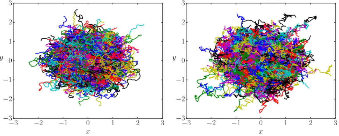
FIG. 3. Colored lines: Sample trajectories according to equations (II.1) and (II.2) for two different noise distributions and vanishing torque. Particle starts at the green dot. Left: α = 0.5 Right: α = 1.5. Noticeable is the different influence of the noise type on the shape of the trajectories. While the trajectory on the left seems to be composed of rather straight lines with sharp turns, the trajectory on the right exhibits more small turns. The black lines correspond to coarse grained trajectories with∆t= 10 = 10τϕ. At the coarse grained level both trajectories follow the same uniform distribution for the directional changes. Other Parameters: Ω = 0
We present in figure 3 as colored lines sample trajectories according to equation (II.1) and (II.2) for vanishing torque and for two different noise types. On the
left α = 0.5 is shown, on the right α = 1.5. Both trajectories have the same relaxation timeτϕ. With decreasing the parameterαthe tails of the respective noise distributions become more pronounced, making sudden large jumps in the velocity direction more and more likely. The peak at the center of the noise distribution becomes more pronounced, so that small changes become less likely. This can be seen in figure 3, if comparing the left and the right picture. The trajectory on the left appears to be composed of rather straight lines with sharp turns, while the trajectory on the right is more wiggling, indicating small turns. The trajectory on the right looks more like a trajectory of an active particle with Gaussian angular driving than the left. The black lines correspond to a coarse grained version of the respective trajectory with a time step ∆t = 10τϕ. At this coarse grained level the trajectories left and right follow the same angular turning statistics. A description of the particle at this coarse grained level is developed in section II A 2. First we will discuss the diffusive properties of the motion of the particle.
1. Mean Squared Displacement And Diffusion Coefficient
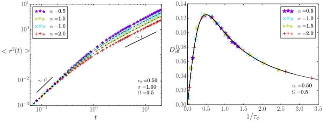
Here we will calculate the mean squared displacement ⟨r2(t)⟩ and determine the effective diffusion coefficientDeff. The results of this section were published in [1]. We consider the particle initially situated at the origin (x(t0), y(t0)) = (0,0) of the Cartesian coordinate system. As the mean squared displacement (MSD) only depends on the distance from the initial position r(t) = |⃗r| =
√x2(t) +y2(t), we can set the initial value ϕ0 = 0. For convenience, we also put t0 = 0. Using the Green-Kubo relation and equation (II.6) the MSD becomes:
⟨r2(t)⟩= 2v20t
∫ t 0
dt′ (
1− t′ t
)
cos(Ωt′) exp (
−t′ τϕ
)
. (II.8)
We integrate over time and introducea= Ω2τϕ2+ 1:
⟨r2⟩= 2v20
⎛
⎝ τϕt
a + τϕ2(
1−Ω2τϕ2)(
cos(Ωt) exp(
−τtϕ)
−1)
a2 +
−
2Ωτϕ3sin(Ωt) exp(
−τtϕ) a2
⎞
⎠. (II.9)
This is the MSD. The time scale τϕ is the crossover time. It separates short time behavior from long time behavior.
To investigate the short time behavior t ≪ τϕ of the MSD, we expand (II.9) up to second order of time:
⟨r2(t)⟩= 2v02
⎛
⎝ τϕt
a +
(τϕ2−Ω2τϕ4)(
−τtϕ +2τt22
ϕ − (Ωt)2 2)
a2 +
−2Ω2τϕ3t(
1− τtϕ) a2
⎞
⎠. (II.10)
⟨r2(t)⟩=v02t2 (II.11) For short times t ≪ τϕ the particle moves ballistic. This ballistic motion is caused by the angular memory or inertia. The persistence length of that motion is
lD =v0τϕ=v0
(v0
σ )α
(II.12) and depends on the noise type through the parameter α.
For times t≫τϕ the motion of the particle follows normal diffusion ⟨r2(t)⟩= 2v02τϕt/a. The effective diffusion coefficient Deff is given by
Deff = lim
t→∞
⟨r2(t)⟩ 4t = v20
2 τϕ
τϕ2Ω2 + 1. (II.13) In the case of Gaussian white noise (α = 2) the result of Weber et al.[56] is
0.0 0.5 1.0 1.5 2.0 2.5 3.0 3.5 1/τφ
0.00 0.02 0.04 0.06 0.08 0.10 0.12 0.14
Deff
v0=0.50 Ω =0.5
α=0.5 α=1.0 α=1.5 α=2.0
FIG. 4. Left: Mean squared displacement for various noise distributions. Symbols from simulations of equations (II.1),(II.2). Dashed line according to (II.9). Param- eters: σ = 1, v0 = 0.5, Ω = 0.5. Right: The effective diffusion coefficient Deff for different noise distributions (α) as a function of the inverse relaxation timeτϕ−1: Simulation (symbols) and theory according to (II.13) (line). Parameters: Ω = 0.5 and v0= 0.5.
recovered and for additionally vanishing torque the result of [54]. For vanishing torque (Ω = 0) the effective diffusion coefficient Deff = v20τϕ/2 = v2+α0 /(2σα) is proportional to the relaxation time and decays with the noise intensity σ as a power law. The power is given by the Lévy stability index α. Expressed through the persistence length (II.12) the effective diffusion coefficients be- comes Deff =v0lD/2.
On the left of figure 4 we show as symbols simulation results of the MSD according to equations (II.1),(II.2) and the analytical result (II.9) as dashed lines. Simulations and theory fit well. The ballistic regime at the beginning and the diffusive regime are clearly distinguishable. Parameters as given in the pictures.
We show on the right in figure 4 the effective diffusion coefficient Deff in de- pendence of the inverse relaxation time τϕ−1 from (II.7). The relaxation time is inverse proportional to theα-th power of the noise strengthσα, so from left to right the noise strength increases. Symbols correspond to simulation results