MARIA S. MERIAN -Berichte
Seamount Observatory and SAMOC Overturning Cruise No. MSM60
January 04 – February 01, 2017
Cape Town (South Africa) – Montevideo (Uruguay)
Dr. S. Speich, S. Asdar, Dr. G. B. Berbel, L. Branlard, A. Carvahlo, DR.
M. P. Chidichimo, Dr. L. Cotrim da Cunha, A. da Silva Calixto, C.
Edsgren, Dr. R. Guerrero, Dr. R. Hummels, Dr. S. Jones, Dr. M.
Kersale, Dr. A. Lebehot, T. Marshall, N. Mohale, A. Rogge, Dr. O. Sato, J. Schrandt, Dr. T. Stöven, B. Sutti Otera
Johannes Karstensen, Dr
GEOMAR Helmholtz Centre for Ocean Research Kiel, Kiel, Germany
2019
Table of Contents
1 CRUISE SUMMARY... 3
1.1 Summary in English ...3
1.2 Zusammenfassung...3
2 PARTICIPANTS ... 4
2.1 Principal Investigators ...4
2.2 Scientific Party ...4
2.3 Participating Institutions...5
2.4 Crew ...5
3 RESEARCH PROGRAM ... 6
3.1 Description of the Work Area ...6
3.2 Aims of the Cruise ...6
3.3 Agenda of the Cruise ...6
4 NARRATIVE OF THE CRUISE ... 7
5 PRELIMINARY RESULTS ... 9
5.1 CTD observations ...9
5.2 Underwater Vision Profiler ... 14
5.3 Water sampling ... 16
5.3.1 Measurements of Salinity ... 16
5.3.2 Oxygen and nutrient samples ... 18
5.3.3 Dissolved Inorganic Carbon and Total Alkalinity ... 19
5.3.4 Total organic carbon ... 23
5.3.5 Nitrogen and oxygen isotope ... 24
5.3.6 Measurements of CFC-12 and SF6 ... 24
5.3.6 HPLC measurements ... 26
5.4 Acoustic Doppler Current Profiler data ... 28
5.4.1 Lowered ADCP ... 28
5.4.2 Ship mounted ADCP ... 30
5.6 Underway data ... 33
5.6.1. Expendable bathythermographs ... 33
5.6.2 Thermosalinograph and meteorological sensor data ... 34
6 STATION LIST RV MARIA S. MERIAN MSM60 ... 36
7 DATA AND SAMPLE STORAGE AND AVAILABILITY... 45
8 ACKNOWLEDGEMENTS ... 45
8 REFERENCES ... 46
1 Cruise Summary
1.1 Summary in English
The scientific program of the MARIA S. MERIAN MSM60 expedition was the first basin-wide section across the South Atlantic following the SAMBA/SAMOC line at 34°30’S. The scientific program consisted of full water depth sampling (up to 5300m) using the CTD/O2/lADCP rosette system. The water samples have been analysed on board for oxygen, dissolved inorganic carbon, alkalinity, salinity, CFC12, and SF6. In addition samples have been taken for later analysis of nutrients, chlorophyll structure (HPLC), POC, and nitrogen isotope analysis. The sampling and measurements where performed against highest standards defined in the GO-SHIP cruise recommendations (http://www.go-ship.org/). An Underwater Vision Profiler (UVP) was mounted on the CTD for full depth particle photography. Underway measurements included hull mounted ADCPs (75kHz and 38kHz) and high resolution (11nm) XBT probes. The data will be analysed for multiple purposes including calculation of the meridional volume, heat, and freshwater transport across the SAMBA/SAMOC line. The biogeochemical data will be compared to historical data acquired at neighbouring sections, e.g. along the WOCE/GO-SHIP A10 section (30°S) occupied by RV Meteor in 1993 as part of the WOCE program. The MSM60 expedition is a contribution to the EU H-2020 AtlantOS project.
1.2 Zusammenfassung
Die Expedition von Maria S Merian MSM60 war die erste Beckenweite GO-SHIP Vermessung des Südatlantiks entlang der SAMBA/SAMOC 34°30’S Linie. Das wissenschaftliche Programm bestand aus 128 CTD/lADCP Profilen mit Wasserprobenentnahme (maximal 22 pro Station) in ausgewählten Tiefen. Dabei wurden die Stationen über die volle Wassertiefe (bis zu 5300m) ausgeführt. Die Wasserproben wurden an Bord für Sauerstoff, gelöster anorganischer Kohlenstoff, Alkalinität, Salzgehalt, CFC12 und SF6 analysiert. Zusätzlich wurden Proben für die spätere Analyse von Nährstoffen, Chlorophyllstruktur (HPLC), partikulären Kohlenstoff, und Stickstoffisotopenanalyse gewonnen. Die Probenahme und Messungen wurden der GO-SHIP Standards (http://www.go-ship.org/) durchgeführt. Ein Underwater-Vision-Profiler (UVP) wurde bei den CTD zur Bestimmung von Partikeln eingesetzt. Die Unterwegs Messungen bestanden aus kontinuierlichen Messungen (ADCPs 75kHz und 38kHz, Meteorologie, Tiefenbestimmung) und diskreten, aber hochauflösende (11nm) XBT-Sonden (331 Profile). Die Datenlage erlaubt es nun Analysen zur Berechnung der meridionalen Volumen-, Wärme- und Süßwasser, sowie Stofftransporte über die SAMBA / SAMOC-Linie durchzuführen Die biogeochemischen Daten werden mit historischen Daten verglichen, die in benachbarten Abschnitten, z.B. entlang der WOCE/GO-SHIP Linie A10 bei 30°S, die beispielsweise von RV Meteor im Jahr 1993 als Teil des WOCE-Programms vermessen wurde. Die MSM60-Expedition ist ein Beitrag zum EU-H2020 AtlantOS-Projekt.
2 Participants
2.1 Principal Investigators
Name Institution
Johannes Karstensen, Dr. GEOMAR
Toste Tanhua. Dr. GEOMAR
Anya Waite, Prof. Dr. AWI/Dalhousie
Edmo Campos, Prof. Dr. IFSP
Sabrina Speich, Prof. Dr. ENS
Rodrigo Kerr, Prof. Dr. FURG
Leticia Cotrim da Cunha, Prof. Dr. UERJ
Ute Schuster, Dr. U Exeter
Isabel Ansorge, Prof. Dr. U Cape Town
Alberto Piola, Prof. Dr U Bueno Aires
2.2 Scientific Party
Name Discipline Institution
Johannes Karstensen Chiefscientist GEOMAR
Rebecca Hummels CTD (processing responsible), lADCP, ADCP GEOMAR
Tim Stöven CFC/SF6 data Quality Control GEOMAR
Julia Schrandt CFC/SF6 CAU Kiel
Caroline Edsgren CFC/SF6 GEOMAR
Andreas Rogge UVP (processing responsible), CFC AWI
Sabrina Speich CTD, Salinometer (processing responsible), supervision training
ENS
Sarah Asdar CTD & station list responsible UCT
Maria Paz Chidichimo CTD, Argo floats responsible SHN
Raul Guerrero CTD/ADCP/IADCP system monitoring INIDEP
Louise Branlard CTD & Real-time data submission UCT
Marion Kersale CTD, ADCP (processing responsible) UCT
Ngwako Mohale CTD, TSG/Underway (processing responsible) UCT
Tanya Marshall CTD, XBT (processing responsible) UTC
Leticia Cotrim da Cunha Carbon, POC responsible UERJ
Olga Tiemi Sato CTD, Salinometer USP
Glaucia B. Benedetti Berbel Nutrient sampling, Oxygen processing responsible
IFSP
Bruno Sutti Otera Nutrient & oxygen sampling IFSP
Andréa Carvalho Carbon, Phytoplankton (HPLC) responsible FURG
Steve Jones Carbon (processing responsible) U Exeter
2.3 Participating Institutions
GEOMAR: Helmholtz Centre for Ocean Research Kiel, Kiel, Germany CAU Kiel: Christian Albrechts University, Kiel, Germany
ENS: École normale supérieure; 45, rue d’Ulm, Paris /France
FURG: Universidade Federal do Rio Grande, Rio Grande – RS, Brasil
IFSP: Instituto Federal de Ciência e Tecnologia de São Paulo, São Paulo, Brasil UERJ: Universidade do Estado do Rio de Janeiro, Rio de Janeiro, Brasil
INIDEP: National Institute Fishery Research & Development, Mar del Plata, Argentina SHN: Servicio de Hidrografía Naval, Buenos Aires, Argentina
UCT: University of Cape Town, University Avenue, Rondebosch, South Africa AWI: Alfred-Wegener-Institut, Am Handelshafen 12, Bremerhaven, Germany U Exeter: University of Exeter, Exeter, Devon, Great Britain
2.4 Crew
Name Rank
SCHMIDT, Ralf Master
STEGMAIER, Eberhard Chief Officer
WICHMANN, Gent 1st Officer
JANSSEN, Sören 2nd Officer
OGRODNIK, Thomas Peter Chief
WOLTEMADE, David 2nd Engineer
SCHWIEGER, Philipp 3rd Engineer
STAAK, Ludwig Ship's Doctor
NEITZEL, Gerd Jürgen Helmut Electrician
HERRMANN, Jens Electronics
REIZE, Emmerich System Operator
WIECHERT, Olaf Klaus Fitter
BOSSELMANN, Norbert Bosun
SIEFKEN, Tobias SM
HAMPEL, Ulrich Bruno SM
THÜß, Anna Katharina SM
PESCHEL, Jens SM
WOLFF, Andreas SM
GRUNERT, Holger SM
BISCHECK, Olaf SM
SAUER, Jürgen Motorman
ARNDT, Waldemar 1st Cook
WOLFF, Thomas 2nd Cook
SEIDEL, Iris Stewardess
3 Research Program
3.1 Description of the Work Area
The current exchange pathways south of Africa and South America drive water mass interactions between the Indian, Pacific, and Atlantic oceans. The Agulhas Current, which flows westward around the southern coast of South Africa, contributes strongly to the upper limb of the Meridional Overturning Circulation (MOC) north-ward flow in the Atlantic Ocean. Additionally, the shedding of Agulhas rings into the eastern South Atlantic is a major source of salinity to the region. The path of deep waters to the Southern Ocean and the Indian Ocean is presumably partitioned between flows along the western boundary and within the Agulhas Undercurrent. In addition, intense mixing in the Cape Basin and the Brazil/Malvinas Confluence are induce significant short-circuits in the MOC. Thus, researchers have identified 34.5°S in the South Atlantic as the latitude most crucial to any examination of how interocean exchange influences the MOC.
3.2 Aims of the Cruise
The aim of the MARIA S. MERIAN MSM60 expedition was to collect for the first time full occupation of a transbasin section along 34.5°S. South Atlantic basin wide ship-based hydrography studies are rare. A few occupations have been done close to 30°S and at 24°S.
Frequent repeats of part occupations of the 34.5°S line have been done on both sides of the Atlantic Ocean (SAMBA off South Africa, and SAMOC off Brazil/Uruguay). Ship-based hydrography is the only method for obtaining high-quality, high spatial and vertical resolution measurements of concurrent physical, chemical, and biological parameters over the full ocean water column. Ship- based hydrography is essential for documenting decadal physical and chemical ocean changes throughout the water column, especially for the deep ocean below 2 km (below the measurements of Argo or XBTs). Hydrographic measurements are needed to:
• reduce uncertainties in global freshwater, heat, and sea-level budgets,
• determine the distributions and controls of natural and anthropogenic carbon (both organic and inorganic),
• determine ocean ventilation and circulation pathways and rates using chemical tracers,
• determine the variability and controls in water mass properties and ventilation,
• determine the significance of a wide range of biogeochemically and ecologically important properties in the ocean interior,
• and to augment the historical database of full water column observations necessary for the study of long-timescale changes.
3.3 Agenda of the Cruise
The scientific program consisted of 128 full water depth profiling and discrete sampling (up to 5300m) using the CTD/O2/lADCP rosette system. The water samples were analysed on board for oxygen, dissolved inorganic carbon, alkalinity, salinity, CFC12, and SF6. In addition samples have been taken for later analysis of nutrients, chlorophyll structure (HPLC), POC, and nitrogen isotope analysis. The sampling and measurements where performed against highest standards defined in the GO-SHIP cruise recommendations (http://www.go-ship.org/). An Underwater Vision Profiler (UVP) was mounted on the CTD for full depth particle photography. Underway measurements
included hull mounted ADCPs (75kHz and 38kHz) and high resolution (11nm) XBT probes. The data is used for multiple purposes, including calculation of the meridional volume, heat, and freshwater transport across the SAMBA/SAMOC line. Argo float (11) were deployed during the cruise.
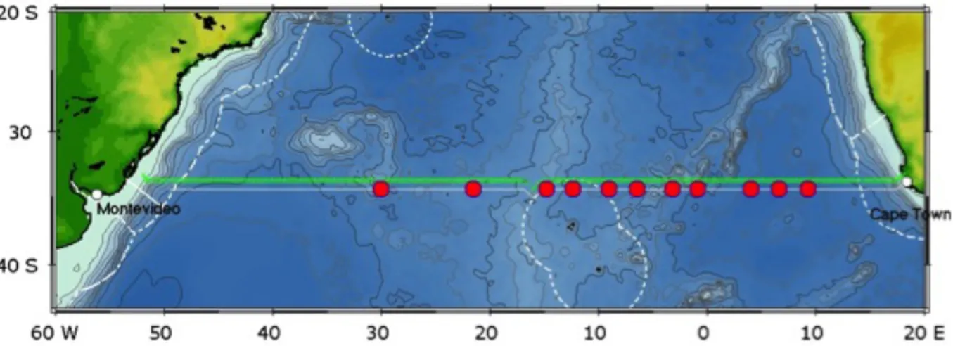
Fig. 3.1 RV Maria S. Merian MSM60 cruise track from Cape Town to Montevideo. Greencrosses dots indicate CTD/Bottle/lADCP casts, red dots indicate Argo float deployments, underway data track (ADCP, TSG) are shown with latitude offset. The EEZ regions are indicated by broken lines.
4 Narrative of the Cruise (J. Karstensen)
Preparatory work for Maria S Merian MSM60 started in Cape Town, South Africa, on January 2nd, early morning. In the late afternoon of January 3rd all science crew member (22), including one Navy observer from Brazil, where on board the ship. Departure was planned January 4th, 08:00, but was delayed because of bunkering was delayed and a dog-squad search of the ship for blind passengers.
Finally we left harbour for the expedition MSM60 on January 4th, 2017 at 14:50 (Local Time). We headed southwest towards our nominal cruise latitude of 34.5°S for a first XBT launch at the 100 m isobaths and a first CTD test station at the 150 m isobath. Unfortunately the CTD at the first test station failed because of a hose that was not removed. We worked our way westward and down the continental slope with XBTs’ launched every 10 nm (later stretched to 11 nm). The CTD sampling was at the boundary about 20 nm, to resolve the more complex current structure we expected here, and later stretched to 33 nm. The first CTD profiles were does with a PAR sensor mounted, but the sensor was removed after the water depth exceeded 2400 m (January 5th). During the first days the CTD cable termination had to be renewed a few times (after CTD st # 13 and
#15) because of an unfortunate combination of wind, currents and waves all coming from different directions the tension cycling was too extreme.
On January 07th we used changed the winch to see if maybe the wire itself was the problem – but that didn’t help much. However, the CTD/lADCP/UVP package could be operated at almost all casts and returned good data. On January 7th we started with sending the XBT and CTD cast data
on a daily basis to Coriolis data centre (France) and to NOAA (USA). We have been approached by a UK group from NOC-Southampton (Brian King) and by EuroArgo to launch a couple of floats along our track. The first of these floats was launched on the January 8th in the Cape Basin.
A few minor problems occurred (ship ADCP communication error, low voltage lADCP) and the seminar talks started on the 9th. On January 10th we had serious problem during CTD #30 – first a shortage at about 600m, followed by a total stop of the system at 3600 m. We tried to restart the application but it failed and we recovered the system and changed the winch (from #2 to #1) again.
A shortage in ship winch cable was detected and a new termination of cable prepared. On January 11th the CTD data acquisition stopped at about 5000 m (upcast). Besides a shortcut in the wire, the data acquisition PC was malfunctioning. Fortunately the WTD team setup a spare PC for us and the system could be used again. We crossed the Greenwich Meridian (January 12th) all systems running, except of a few problems with the CTD release pylon that controls the bottle sampling.
Again the WTD/electronics help us by trying to exchange our with the Maria S Merian own pylon – however, that did not work at all and we changed back to the old (malfunctioned) system.
We crossed the Walvis Ridge (14th), which separates the Cape Basin from the Angola Basin, and water depth changed drastically by more than 3000 m over a distance of 15 km only. On January 17th we headed to more than half a degree south in order to recover a BioArgo float owned by French colleagues from Villefranche. The float was drifting since October 2016 (shortly after deployment) for unknown reasons. Because it was to rough seas or a Zodica recovery, the crew designed a recovery tool that proved to work well and the float was on board at 18:40 LT. We then headed back to the nominal latitude 34.5°S of our SAMBA/SAMOC section. A short report was written about the recovery (incl. the tool) and send to JCOMM. Because Argo drifter are nowadays more frequently equipped with additional (expensive) sensors it is getting increasingly attractive to recover floats to re-use and recalibrate the sensors.
A topographic survey of the Ridge system close to the Rio Grande Rise was performed on January 22nd. The Ridge is an important obstacle for the flow of Antarctic Bottom Water. Towards the end of the MSM60 expedition we started with preparations not only for the leaving the ship but for the reception that was kindly arranged by the captain and the German embassy in Montevideo on February 1st. All groups on board prepared a poster presentation. On January 30th we entered into Brazilian EEZ and the EM122 was stopped because we did not apply for permission to use the device in Brazilian waters. On January 31st the last CTD station (#128) was done at 130 m water depth and a last XBT (#331) at 100 m. We stopped underway data acquisition when entering the Uruguayan EEZ. The reception took place a couple of hours after we moored in Montevideo old town harbour.
5 Preliminary Results 5.1 CTD observations
(R. Guerrero, R. Hummels)
CTD/Rosette we used during MSM60 had been transferred from RV Meteor were it was used for two legs. From mid December to port call Maria S Merian on the 1st January 2017 the CTD was in a storage place in Cape Town. Most part were already mounted and set-up, wires were connected and we tested the rosette sampler, added sensors, tested the Electro Mechanical cable (EM cable) etc. For the MSM60 expedition the CTD assembly was composed of: A SBE-9 CTD profiler, a SBE-32 carrousel for water sampling, 22 Hydro Bios 10 liters niskin bottles, an Hydroptic Underwater Vision Profiler (UVP), two RDI-Teledyne 300 kHz L-ADCP (upward and downward looking) and additional sensors (see Fig. 5.1).
Fig. 5.1: (Left) Protective cage containing the CTD (hided), Bottles and L-ADCP array. (Right top and bottom) Distribution of sensors connected to the CTD (except the UVP that was autonomous).
L-ADCP units were also self-contained.
Data acquisition via the SBE11 deckunit, was done using two PC: First the GEOMAR PC
“SpermWhale “ was sued but that failed after half of the cruise and a PC provided by the ship was used after. The SBE based CTD data processing was done immediately after each cast running batch file.
Table 5.1: Summary of CTD system configuration on Maria S Merian MSM60.
System Sensors Model Serial N Calib. date
Primary Temperature SBE3 plus 4831 22-Apr-16
Conductivity SBE4c 2452 06-Mar-13
Oxygen SBE43 0631 19-Mar-16
Pump SBE 5T 4750 -
Secondary Temperature 1 SBE3 plus 5628 16-01-13
Conductivity 1 SBE4c 4096 15-01-13
Oxygen 1 SBE43 2416 12-01-13
Pump 1 SBE 5T 4748 -
Auxiliary PAR/irradiance1 Biospherical/Licor 4716 17-Oct-16 Transmissometer WetLab C-Star 1617 DR 05-Apr-12 Flu-Turb. WetLabs Eco AFL/FL 2294 12-Oct-11
Altimeter Benthos PSA 916 41840 -
UnderW Vision Prof. HydropticV5HD 202 06-12-16 Pressure SBE9plus DigiQuartz 75760 07-Sept-99
Rosette Hub assembly SBE-32 0342 -
Deck Unit SBE11 plus - -
Surface irradiance SPAR 20195 10-Mar-16
Bottles 24-10 ltrs bottles Hydro-bios (Kiel) - -
CTD sensor behavior
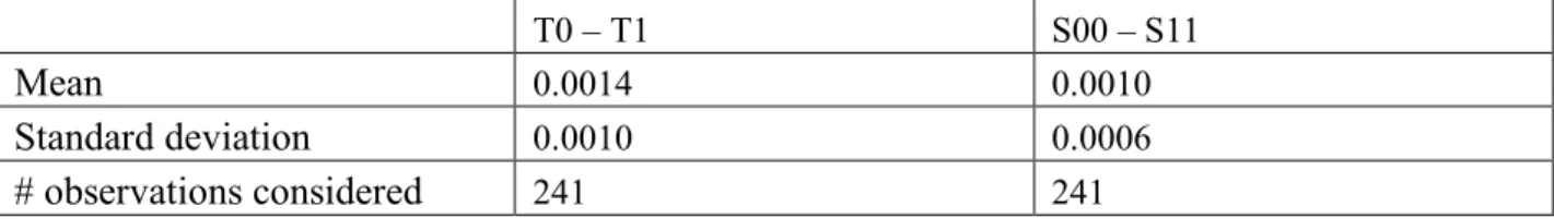
The CTD instrument was equipped with redundant sensors for temperature, conductivity (salinity) and oxygen. To obtain a first impression on sensor behavior (before calibration) a comparison of parallel data records was routinely done. The difference, based on the SBE generated BTL files using every 5th station shows good agreement (Tab. 5.2).
Table 5.2: Statistics of Temperature and Salinity (conductivity) sensor comparison for pressure higher than 1000 db. and a subsample of stations along the cruise (stations 5 to 125 every 5 were chosen).
T0 – T1 S00 – S11
Mean 0.0014 0.0010
Standard deviation 0.0010 0.0006
# observations considered 241 241
Niskin bottles and Rosette sampler
1 The surface PAR sensor (Spar Biospherical; SN 20195; calib: 10-03-16), connected to the SBE11 Deck Unit, was provided by the ship.
SBE carrousel was showing erratic failures in closing bottles but for most no systematic miss releasing was observed. The trigger release mechanism was disassembled and triggers changed.
From thereon a thoroughly high pressure flushing on the release mechanism with fresh water became a routine maintenance procedure. By station #43, 21 bottles failed to release and Kiel-SN 0342 unit was exchanged with the Maria S Merian CTD unit (MSM-SN0548) but the system failed completely (even thought it worked well on deck) for unknown reason. At station #46, the MSM- SN0548 was changed with another MSM hub assembly but that did not resolve the problem and at station #47 the original Kiel-SN 0342 was re-installed and we continuous operating the rosette having miss-fired bottles. In total (128 stations) we had 112 miss firing:
47 x btl#8, 22 x btl#19; 9 x btl#10. 7 x btl#21. On Station 112 bottle # 19 was lost but no obvious reason was found.
Leaking on bottles was observed mostly on the first stations. In all cases the leakage occurred at the lower cap. When this occurred the O-rings were checked for damage or uneven sitting of them on the bottle notch. Leaking bottles were (stn#/bottle#): 3/4, 4/10, 8/6, 32/9, 34/5-7-15, 37/9-15, 38/9-5-15, 49/9, 50/5, 63/9-15, 65/6, 66/7, 67/15, 87/22 and 93/22. Station 101 went down with all the air vents OPEN.
On every station, the CTD assembly was lowered between 5 to 15 m off the bottom, depending on weather and rolling conditions. On station 17 there was not approach as the watch standing had uncertain bottom depth information from the ship eco-sounder. On stations 48 and 98 the CTD assembly reached the bottom of the sea at a lowering speed of 1 m/s. On station 48 there was a misreading on the sonic depth and the real bottom depth was shallower than expected. On station 98 it was caused by distraction on the watch standing. No damage on the CTD assembly was observed nor in any of the sensors.
Inductive cable twisting
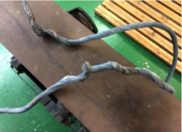
On station 13, 15, 16 and 82 the EM cable showed moderate to severe kinking immediately above the CTD assembly (first 5 m) (Fig. 5.2). Those stations were executed under 30 to 40 knots wind.
Even though the ship was maintaining proper position relative to the wind direction, the large rolling amplitude were transmitted to the CTD assembly causing the twisting of the cable.
Fig. 5.2: Twisted cable (st. 13, 15 and 16)
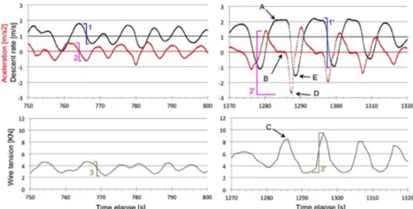
Using the descent rate and acceleration the CTD was constantly monitored and the stress on the cable during the cast was evaluated in real-time. We learned from station where problems occurred (e.g. CTD 13 shown Fig. 5.3) the critical parameters to watch for.
Fig. 5.3: Station 13: (left) normal behaviour and (right) event that lead to damage in cable. During normal behaviour the CTD was lowered with 1 m/s, but oscillating between 0.5 and 1.8 (1) with the acceleration between -0.5 to + 0.5 m/s2 (2). The tension on the cable shows changes of about 2.3 KN (3). During an event significant larger amplitudes in all three parameters occur: 3.1 m/s change in descent rate (1’), the acceleration going from 1.4 to -2.8 m/s2; a change over 4 m/s2 (2’). And the tension in the cable goes from 2.8 KN (probably the weight of cable) to 9.5 KN in two second (3’) .
It is of general knowledge among CTD groups that under rolling conditions kinking on the wire could occur when:
- the downward velocity of the wire (winch speed + rolling speed) exceed the free fall velocities of the CTD assembly (point A on figures) . Then the wire goes slack on top of the package (point B on figures)
- if there is any twist in the slacked cable.
- then the slag is suddenly taken by the rolling in the opposite direction (point C on figures).
In our case the free fall velocity of the CTD package (when descending) is 2.1 m/s (Fig. 5.4 top- left). The slack condition of the cable should occur during B (4 s with 0 acceleration and the which going at 1 m/s). Sudden rolls of the ship in the opposite direction (point C) takes all the slack up in around 2 seconds not giving enough time for the wire to un-twist.
Seasoft failure
Seasoft stopped acquisition on stations 30, 33, 74, 75 and 100. On station 30, after having a large offset in all sensor at 594 db, the Seasoft indicated communication time out; the acquisition was re-started but failed.
CTD Processing
After the calibration using the SBE scripts the CTD preprocessed data was merged with the bottle data (oxygen, salinity) and a calibration of the conductivity and oxygen sensor followed.
Conductivity was calibrated using a linear relation in P, T and C. The resulting rms salinity misfit was 0.00126 psu and 0.00139 psu for the sensors 1 and 2 respectively after removal of the most deviating 33% of samples.
Oxygen was calibrated using a relation linear in P, T and O. Winkler titration bottle samples led to a relation with an rms misfit of 1.0944 µmol/kg and 1.0858 for sensor 1 and 2 respectively (33%
of bottle values removed). Further sensors were attached to the carousel and recorded, but were not further calibrated: a fluorescence and turbidity sensor (Wetlabs), and a Photosynthetically Active Radiation (PAR) sensor (Biospherical). The latter could only be used on casts less than 2000 m deep. An altimeter worked during the entire cruise and was used for the bottom approaches.
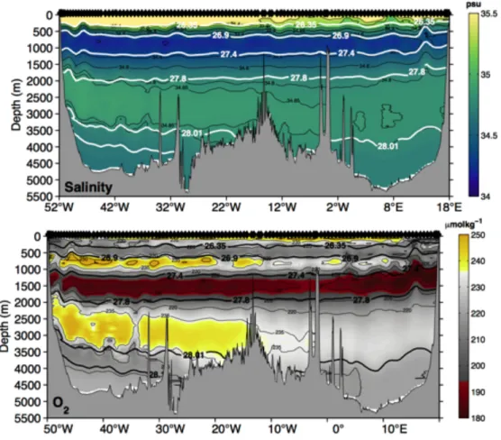
Fig. 5.4 Salinity (upper) and oxygen (lower) distribution along the SAMOC/SAMBA section with dedicated potential density anomaly contours overlaid.
A first view on the section data (Fig. 5.4) nicely shows the signatures of different water masses in salinity and temperature. A clear separation between the eastern and western basin and water masses entering from the north (oxygenated Deep Western Boundary Current signature) and south Circumpolar Deep Water and Antarctic Bottom Water (west, below 4000m). Antarctic Intermediate Water (salinity minimum centered at 1000m depth) show a zonal gradient.
5.2 Underwater Vision Profiler (A. Rogge)
The Underwater Vision Profiler (UVP), an optical system for particle counting and imaging, was used during Maria S Merian MSM60 cruise to quantify particle abundances and to identify planktonic organisms in the South Atlantic Ocean.
The UVP was used to measure abundances, size distributions and grey levels of particles and planktonic organisms larger than 0.015 mm² in diameter throughout the water column. It consists of a camera, which acquires images of a defined area between two rows of red light emitting LEDs with a frequency of 20 Hz and is thus able to calculate particle profiles related to a pressure sensor.
Additionally, the UVP was programmed to store images of single particles larger than 0.62 mm².
The device was inter-calibrated at the Laboratoire de Oceanographique de Villefranche-sur-mer (LOV, France) in December 2016, right before the cruise to ensure comparable results with other units all around the world.
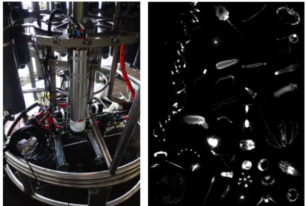
The UVP was mounted onto the water sampler rosette (Fig. 5.5) and operated in “Pressure mode”, except during the last shallow (< 75m) stations. Pressure mode allows the device to start and stop acquisition autonomously. After reaching the CTD flushing depth at 22 m it starts acquisition and shuts down when the CTD is ascending more than 30 m. This reduces the amount of not usable data from flushing (upper part of profile) and ascending to reduce the amount of data and to saves battery power. Due to the integrated pressure sensor it is later possible to merge the UVP records with the CTD records.
Fig. 5.5: The Underwater Vision Profiler and first plankton images. (left) UVP mounted on the CTD rosette and (right) image collection of organisms.
Preliminary results and further data processing
We were able to measure 138 profiles down to a maximum depth of 5569 m and to acquire about 480.000 images (selected ones in Fig. 5.5, left).
Total particle numbers show enhanced particle abundances above the continental slopes and above seamounts (Fig. 5.6). Very interesting is also the high amount of bigger particles at the continental slope off South American. Future analysis will include a combination of small particle (<0.62 mm²) abundances and volumes with water masses (based on CTD and transient tracer data). This allows the implementation of oceanographic features as eddies and upwelling to show fundamental effects and to calculate export rates.
Furthermore, the semi-automatic analysis software Ecotaxa will be used to identify and quantify planktonic organisms and aggregates in the acquired vignettes.
Fig. 5.6: UVP records along the SAMBA/SAMOC line. (upper) Small particles (< 0.62 mm²) occurrence per litre, and (lower) particle size as top view area in number of pixels per litre.
5.3 Water sampling
5.3.1 Measurements of Salinity (S. Speich, O. Sato)
During the cruise, two different Salinometers were set-up: A Guidline Portasal Salinometer 8410A and an OPTIMARE Precision Salinometer (OPS). Before starting the analyses of the water samples from the Rosette Niskin Bottles, we performed comparisons between the two salinometers analyses and procedures and concluded the following:
1. As indicated in the OPS Operating Manual, we proceeded to the salinity bottle warming in a water bath at about 39°C - 40°C temperature. When the salinity water samples were warmed enough, we shacked them energetically and immediately after that we slightly opened the stopper of the bottles and closed it again to enable the air under pressure after warming to escape from the sample. In the OPS Operating Manual, a slightly different procedure is described, using a needle on butyl stoppers to extract the air. However, our sampling bottles were not provided with such stoppers but instead with the very practical beer top that have a rubber cushion that can be opened only slightly to make the air to come out without a massive air exchange. We left the water samples to cool down to the Salinometer room controlled temperature and we shacked them again and making once more escape some aire before sampling them with the salinometer.
2. This procedure has shown to reduce dramatically the variability in both salinometers measurements and consequently the time for each sample measurement. This is very likely due to the removal, by this procedure, of most of the micro-gas bubbles, particularly present in the deep cold waters that impacts the conductivity measure.
3. With the OPS, the processing of the water sample is automated in that a the user-initiated start the instrument continues the complete analyses without further interaction. Rinsing, repeated sampling, and flushing are performed automatically. Main process parameters like the number of rinsing cycles and repetitions of measurements are adjustable.
4. The OPS has a temperature-controlled pre-bath. This is very efficient as it is used to further adjust the temperature of the water sample. Thus, the pre-bath prevents the transfer of heat into the main bath. It is not necessary to wait for a pre-adjustment of the temperature of the water samples. This guarantees rapid sample evaluation of water samples.
5. The OPS has a comprehensive set of housekeeping data that is continuously recorded to ensure that the measurement is always fully documented. Moreover, plausibility checks are performed continuously. The temperature of the main bath is determined with a precision of one milliKelvin and recorded together with the conductivity of the water sample, leading to an accuracy of better than 0.001 Equivalent Practical Salinity Units (PSU).
Because of points 2 to 4, we decided to use the OPS for analyzing the salinity samples throughout the Maria S Merian MSM60 cruise. Indeed, the measures when the bottles were warmed and micro-air bubbles released were very stables and the built-in computer insured a complete documentation of all the processing and results, preventing, in addition, any “human”
error.
We analyzed 5 to 8 samples per CTD station, that is a total of about 1000 samples. The sampling depths were chosen to cover the most prominent features in the water column, with a
particular emphasis given on deep bottles as there properties of seawater vary less and therefore they are more indicated for the CTD conductivity sensors calibration.
To calibrate the Salinometer measurements we used both, OSIL Standard water samples and Substandard home-made water samples. The latter are made by filling the usual salinity seawater bottles, with the “same” sea water. This was collected at four different times from the deepest Niskin bottles and mixed in a 25 L jar. The substandard water underwent to the same procedures of heating and degasing as any other samples of seawater.
Because we noted a drift in the standard water measurements during few days, we performed three times (at different days) a standardization procedure. To be noted here that we did not heat and degas any of the standard water samples. The OPS log files provide the slopes corrections computed for each standardization procedure.
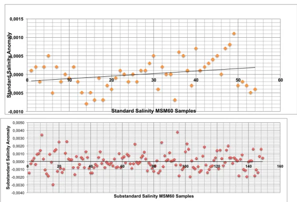
Standard and Substandard water samples give the accuracy of the salinity measurements we performed. The results are depicted in terms of anomaly from computed means for each box of samples of standard and substandard waters (Fig. 5.7). The computed Standard Deviation for Standard Water is 4 10-4 PSU and for Substandard Water is 1.1 10-3 PSU.
Fig. 5.7: (Upper) Distribution of MSM60 Standard Water anomalies. (Lower) distribution of MSM60 Substandard Water anomalies. The linear regression lines are superimposed in each graphic.
-0,0010 -0,0005 0,0000 0,0005 0,0010 0,0015
0 10 20 30 40 50 60
Standard Salinity Anomaly
Standard Salinity MSM60 Samples
-0,0040 -0,0030 -0,0020 -0,0010 0,0000 0,0010 0,0020 0,0030 0,0040 0,0050
0 20 40 60 80 100 120 140 160
Substandard Salinity Anomaly
Substandard Salinity MSM60 Samples
5.3.2 Oxygen and nutrient samples
(G. B. Benedetti Berbel, B. Sutti Otera)
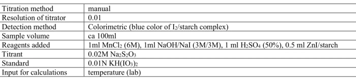
For oxygen analysis water samples have been collected from the rosette and titrated onboard using a GEOMAR, Kiel provided titration system (Tab. 5.3). The chemistry method behind goes back to Winkler (1888). The system uses a colorimetry method for analysis considering sample volume and concentration of reagents.
Tab. 5.3.: Winkler system onboard MSM60
Titration method manual
Resolution of titrator 0.01
Detection method Colorimetric (blue color of I2/starch complex)
Sample volume ca 100ml
Reagents added 1ml MnCl2 (6M), 1ml NaOH/NaI (3M/3M), 1 ml H2SO4 (50%), 0.5 ml ZnI/starch
Titrant 0.02M Na2S2O3
Standard 0.01N KH(IO3)2
Input for calculations temperature (lab)
It is crucial to take the water samples without air bubbles. Immediately after taking the sample Mangan(II)-chloride (MnCl2) and Sodium-Iodide (NaI) are added and stirred by thorough-fully shaking. Due to the instability of MnCl2 in alkaline solutions alkaline NaI is added at the same time and thus increases the efficiency of the reaction. After at least 30 minutes in the dark the precipitation should have settled and the sample can be titrated. The iodide ions added with the NaI are oxidized to iodine by the manganese(III) ions which are reduced to manganese(II) ions.
In the last step, the iodine is titrated with sodium thiosulphate. Thereby, the iodine is reduced to iodide thiosulphate in turn is oxidized to tetrathionate ions. Since the turning point from yellow to colorless is difficult to see, a starch solution (in our case a zink-starch-solution) is added which induces a dark blue color. Since the sodium thiosulphate slowly deteriorates its proportions have to be determined once per day before or after the measurements. The standardization of thiosulfate solution was conducted with 3 to 5 titrations on every sampling day and when a new solution was prepared.
Samples were collected immediately after the CTD rosette was put on deck. A piece of Tygon tube was used to transfer the samples from Niskin bottles into vials. The sample vials were flushed 2 to 3 times their volume. Special care was taken to avoid bubbles in both the tube and the vials.
Samples were immediately pickled with the MnCl2 and NaOH/NaI reagents, the stopper was dropped in place and the vials were vigorously shaken several times to ensure the reactions between water sample and reagents were completed. Blank reagents were run whenever a new batch of reagents was prepared…
Despite following the recommended procedures for oxygen titration (GoShip reference) the comparison of titration results with CTD SBE43 readings showed systematic and grouped (in reference to stations number) varying biases that roughly align with the preparation of a new standards. This suggests that the standards were not properly prepared. For the final data we decided to replace individual standard values the mean of all standards. This procedure lowered the RMS and, more importantly, resulted in the noise being more “white noise” like and unstructured. When comparing the so calibrated CTD oxygen with climatological and other data
(Cape Verde observatory, MSM61) revealed very good agreement. However, as a consequence of the shortcoming in the titration process the standard error for the CTD data was increased.
Nutrients
Nutrient samples were collected in 10 mL vials and then frozen to -80°C for preservation and after about 1 day transferred to a -20°C freezer for storage. The sampled where shipped with Maria S Merian to Kiel. Analysis of these samples has been done in GEOMAR in May/June 2017. The analysis, as well as the sampling, included training of Bruno Sutti (USP) through a AtlantOS WP8/POGO training grant.
It turned out that the sampling and in particular the freezing was not done with sufficient care. The instructions on proper sampling were not always followed, in particular the required headspace of 10% of the vial volume was not followed. The whole batch of data was of very mixed quality and finally it was decided, after several quality control efforts that the nutrient data is not usable.
5.3.3 Dissolved Inorganic Carbon and Total Alkalinity (S. Jones, A. Lebehot, L. Cotrim da Cunha, A. de Oliveira ) Sampling procedure
The Marine Carbon Biogeochemistry Group conducted the measurements of Dissolved Inorganic Carbon (DIC) and Total Alkalinity (TA) on board. All water samples for DIC and TA analysis were sampled according to the recommendations of the Standard Operation Procedure #1 (SOP#1) (Dickson et al., 2007). Once the rosette with the Niskin bottles was on deck, samples were taken as fast as possible – preferably within 10 minutes after the arrival of the rosette on deck, and before the Niskin bottles are half-empty – in order to minimise any potential exchange with the surrounding atmosphere.
Samples were carefully taken from the Niskin bottles using glass bottles (borosilicate glass) and a Tygon tube, which avoided any formation of bubbles. The glass bottles were rinsed twice, overfilled by twice their volume and immediately closed with their corresponding glass stopper.
We then removed 1% of the bottle’s volume using a pipette, to allow for water thermal expansion.
To stop any biological activity and hence affecting the DIC concentration, samples were poisoned with 0.02% of the bottle’s volume of saturated mercuric chloride (HgCl2).
In total, 128 stations were occupied along the 34.5°S section using a rosette holding 22 Niskin bottles of 10 litre capacity. Seawater for DIC and TA analysis was collected at each station, for all depths (i.e. from the 22 Niskin bottles - if all successfully closed). Specifically, 4 samples were taken in 500ml bottles (top, bottom, plus two random bottles in between) to allow duplicate analysis, and the other samples were taken in 250ml bottles.
Due to time constraints, we analysed samples co-located with changes in the water mass distribution based on the CTD temperature, salinity and oxygen profiles, and at selected depths between stations to optimise spatial interpolation throughout the whole section. The bottom and surface samples were always included in this sub-set selection of analysed bottles. The unanalysed bottles were kept aside for possible future analysis.
For each station, once our sub-set selection of samples analysed, we completed a first quality control and identified important gaps in the DIC and TA profiles or possible interesting features or outliers. Samples from these locations were analysed and added to the results where time permitted. The remaining samples, that would not significantly improve the DIC and TA profiles, were discarded.
The total amount of collected samples was 2,601, and the final number of analysed samples was 1,738 for DIC and 1,764 for TA (the difference is due to some failed analyses).
Methods
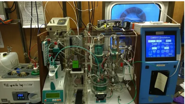
DIC was analysed by coulometry (Johnson et al., 1987, 1993) following SOP#2 (Dickson et al., 2007) and TA by potentiometric titration (Mintrop et al., 2000) following SOP #3b (Dickson et al., 2007). For both DIC and TA, two Versatile Instruments for the Determination of Titration Alkalinity (VINDTA, Marianda, Kiel, Germany, serial numbers #064 and #065 – Figure 5.8), connected to a coulometer (UIC, Inc., Joliet, Illinois, USA) and a Titrino (Metrohm, Herisau, Switzerland) were used.
Fig. 5.8 VINDTAs in the Marine Biogeochemistry container from the University of Exeter, on board FS Maria S Merian.
During the cruise, both VINDTAs calibration was conducted using Certified Reference Material for DIC and TA (CRMs) batch 159 (Prof. A Dickson, Scripps Institution of Oceanography, University of California San Diego, USA). Specifically, we analysed 3 CRMs for each coulometric cell: one at the beginning once the new cell was settled, one at ~12 hours and a final one at the end of the cell’s lifetime (at ~ 24 hours). Each CRM was analysed as a replicate to ensure that the VINDTAs were running reliably.
Analysis on the replicate samples (using the 500 mL bottles) allowed us to conduct a precision study (Figure 5.9) and also identify potential issues with the machine, sensors or chemical, which were then immediately solved. Following SOP 22, from Dickson [2007], the mean difference between replicates was used to calculate warning limits and control limits. Approximately 95% of
replicates should be within the warning limit, and few should be outside the control limit. Table 5.4 shows the limits calculated for the two VINDTAs instruments during the cruise.
Table 5.4: Warning and Control Limits for the VINDTAs. All values are in µmol/kg.
Variable Machine Mean Warning Limit Control Limit % within WL % outside CL
DIC 64 2.81 7.07 9.19 93.61 2.74
65 5.84 14.66 19.07 92.64 1.84
TA 64 1.22 3.06 3.98 92.31 2.71
65 1.13 2.84 3.69 92.53 5.17
Fig. 5.9 - Analysis of DIC and TA replicates. Top: first vs. second replicates for (a) DIC and (b) TA.
Blue and red values are from instrument 64 and 65 respectively. Bottom: Frequency of differences between replicates for (c) DIC and (d) TA. Dashed lines indicate from left to right the mean, warning limit and control limit for each machine (Table 1). Blue (red) indicates machine 64 (65).
Throughout the cruise, no major technical issues on the VINDTAs occurred. Minor changes are reported below for both VINDTAs:
VINDTA #064: The input water lines in Valve 6 have been swapped due to an air leak at the join between the inside and outside part of the machine (line 2 is used when the software selects line 1). On 18th of January, the light bulb on the coulometer intermittently went out. Although nothing particularly explained this issue, the bulb was replaced, and no further problems were seen.
VINDTA #065: Since the temperature sensor for line 1 was faulty, we swapped the temperature sensors of line 1 with the temperature sensor of line 2. On 18th of January, due to faulty detection from the sensor at the base for the AT pipette, the tube connecting to the alkalinity cell has been
changed. This tubing change leads to change in the AT volume, which will need to be recalibrated.
We therefore have taken the new volume of ionised water using 15 calibration bottles, that have been weighed prior to the cruise. The filled calibration bottles will be weighed again back at the University of Exeter to determine the new AT pipette’s volume.
The majority of samples collected were subjected to 1st level quality control whilst on board, allowing any technical, instrumental, and analytical issues (precision) to be addressed immediately. The remaining 1st level quality control will be conducted post-cruise (for the last sampled stations - 30th Jan and 31st Jan 2017).
When back at the University of Exeter, Dr. Ute Schuster’s group will perform a complete 2nd level quality control on all samples using a crossover analysis toolbox provided by Lauvset and Tanhua (2015) in order to assess the accuracy of the measurements (Figure 5.10). This analysis tool box is available for download at CDIAC: http://cdiac.ornl.gov/ftp/oceans/2nd_QC_Tool_V2/ .
Fig. 5.10: DIC (top) and TA (bottom) section across 34.5°S, both in µmol/kg. The analysed sample values have
been interpolated using the Ocean Data View software [Schlitzer, 2017].
5.3.4 Total organic carbon (L. Cotrim da Cunha)
Organic carbon (TOC) is produced in the surface ocean via biological processes (e.g. primary production). In this area of the South Atlantic Ocean (34° 30’ S), the dynamic circulation processes are probably affecting its vertical distribution and thus helping to “pump” organic carbon – formed in the spring and summer periods in this region – from the surface to deeper layers of the ocean.
In order to assess the synoptic distribution of total organic carbon along the SAMOC/SAMBA line, samples were collected at every 5th station (circa every 3° longitude – Figure 5.11), at all depths. Here we’ll refer to organic carbon as “total” because the samples weren’t filtered (TOC).
Total organic carbon is the remaining carbon in a water sample after the removal of all inorganic carbon by acidification and sparging of the sample.
The samples were taken from the Niskin bottles at the selected stations straight after the collection of DIC/TA samples, and stored in glass or HDPE 60 mL flasks, previously cleaned with HCl 0.1N and deionised water at the Chemical Oceanography Laboratory at UERJ. All flasks were immediately frozen, and kept at –20°C during the cruise. In total, 479 water samples were taken in 27 stations. The samples are staying onboard FS Merian until its arrival in Germany. Analysis will take place in the Chemical Oceanography Department of the Helmholtz Institute for Marine Research – GEOMAR, Kiel, Germany. This is part of a cooperation project between Prof. Leticia Cotrim da Cunha and Dr. Tobias Steinhoff (GEOMAR) established in 2015.
The analysis method follows the recommendations of SOP#7 (Dickson et al. 2007). All remaining carbon after acidification of the sample with hydrochloric acid (“non-purgeable organic carbon”) is combusted at high temperature, and then converted into CO2, which is detected by a non- dispersive infrared detector (NDIR) in a TOC-Shimadzu Carbon analyser.
Fig. 5.11 Section map with the TOC samples location during MSM60.
5.3.5 Nitrogen and oxygen isotope (T. Marshall)
Sampling water was collect from every second CTD cast throughout the cruise. The total number of stations sampled is 61. From every niskin bottle two samples were collected to create duplicates.
Following sample collection each sample bottle was immediately filtered through a 0.2 micron filter and then frozen at -20 °C. When samples could not be filtered immediately, they were stored in a -20 °C before filtering. Isotopic sample analysis will take place in Geesthacht, Germany following the cruise. The completion of the analysis is expected to be September 2017. The isotopes comprising of nitrogen and oxygen, will be analysed.
5.3.6 Measurements of CFC-12 and SF6 (T. Stöven)
Analysis System Setup
During the cruise, a gas chromatographic - electron capture detector system was used in connection with a purge and trap unit (GC-ECD/PT5) for the measurements of the transient tracers CFC-12 and SF6. The systems is a modified version of the set-up normally used for the analysis of CFCs (Bullister and Weiss, 1988).
The trap consisted of 100 cm 1/16” tubing packed with 70 cm Heysep D kept at temperatures between -60 and -68°C during the purge and trap process. The traps were desorbed by heating to 110°C and injected onto a pre-column of 20 cm Porasil C followed by 20cm Molsieve 5A in a 1/8” stainless steel tubing. The main column consisted of 1/8” packed stainless steel tubing with 180 cm Carbograph 1AC (60-80 mesh) and a 50 cm Molsieve 5A post-column. All columns were kept isothermal at 50°C. Detection was performed on an Electron Capture Detector (ECD). This set-up allowed efficient and simultaneous analysis of both tracers.
Samples were drawn from Niskin bottles using 250 ml ground glass syringes, of which an aliquot about 200 ml was injected to the purge-and-trap system. The sampling strategy was based on full depths profiles with 22 specific depths. The sampling depths were chosen to cover the most prominent features in the water column such as biological features and characteristics of certain water masses.
Standardization was performed by injecting small volumes of gaseous standard containing SF6
and CFC-12. This working standard was prepared by the company Deuste-Steiniger (Germany).
The CFC-12 concentration in the standard has been calibrated vs. a reference standard obtained from R.F Weiss group at SIO, and the CFC-12 data are reported on the SIO98 scale. Another calibration of the working standard will take place in the lab after the cruise. Calibration curves were measured roughly once a week in order to characterize the non-linearity of the system, depending on work load and system performance. Point calibrations were always performed between stations to determine the short term drift in the detector. Replicate measurements were taken on several stations for data statistics. The final processing and calibration of the obtained transient tracer data will be performed onshore at the GEOMAR in Kiel.
Preliminary results
The distribution of CFC-12 and SF6 along 34°30’S describes the specific ventilation pattern of the different water masses (Fig. 5.12). The different distribution of both tracers is based on their different atmospheric histories so that CFC-12 already covers the deeper and less ventilated water masses whereas the detection limit of SF6 is reached at ~1500m. Both tracers show features from cyclonic eddies at 16°E and 23°W which can clearly be seen by the low tracer concentrations extending almost to the surface. The bottom water east of the mid-Atlantic ridge shows Antarctic Bottom Water (AABW) indicated by the elevated CFC-12 concentrations (not visible in color coding of Fig.1). The bottom water west of the ridge also contains SF6 , although close to the detection limit, which means that the Antarctic Bottom Water (AABW) in this area is more recently ventilated than on the east side of the ridge. The the North Atlantic Deep Water (NADW) is characterized by an absence of SF6 and the lowest CFC-12 concentrations and is thus the lowest ventilated water mass in this ocean area.
All sections are an important contribution to the transient tracer data collection. The analysis of ventilation processes by transient tracers provide further information such as the anthropogenic carbon column inventory, i.e. the carbon uptake by the ocean, and the oxygen budgets in the ocean, especially in the oxygen minimum zones. Furthermore, transient tracer time series of such repeat hydrography sections in the Atlantic Ocean allow for additional investigation on changes in ventilation and the adjoining parameters – a powerful tool to record the impact of climate change on the worlds ocean.
Fig. 5.12: Distribution of SF6 (upper panel) and CFC-12 (lower panel) partial pressure along 34°30’S
5.3.6 HPLC measurements
(L. A. de Carvalho, C.R.B. Mendes, R. Kerr) Sampling
A total of 109 seawater samples at the deep-chlorophyll maximum (DCM) are taken from the 84 CTD (conductivity–temperature–depth) castings for further analysis of phytoplankton pigments through the high performance liquid chromatography (HPLC; (Table 1). The DCM depth was selected based on fluorescence profiles obtained by an in vivo chlorophyll fluorescence sensor (WetLabss profiling fluorometer). Additionally, at some coastal stations (see Table 5.5), seawater samples were also taken from sea surface to better characterize the vertical distribution of phytoplankton communities.
Discrete water samples (1–2 L) were filtered onto 25-mm glass fiber filters (Whatman GF/F- nominal pore size 0.7 µm and 47 mm diameter) under a vacuum pressure lower than 200 mmHg using a TECNAL vacuum pump (model TE-058) for later HPLC pigment analysis. The filters were kept frozen at –25°C during the cruise and conserved frozen until arrival at the laboratory.
HPLC pigment analysis
Phytoplankton pigments were analyzed in the ‘Laboratory of Phytoplankton and Marine Microorganisms’ at Federal University of Rio Grande (FURG), Brazil. The filters were placed in a screw-cap centrifuge tube with 3 mL of 95% cold-buffered methanol (2% ammonium acetate) containing 0.05 mg L–1 trans-β-apo-8'-carotenal (Fluka) as an internal standard. Samples were sonicated for 5 min in an ice-water bath, placed at –20 °C for 1 h, and centrifuged at 1100 rpm for 5 min at 3°C. The supernatants were filtered through Fluoropore PTFE membrane filters (0.2 µm pore size) to rid the extract from the remains of filter and cell debris. Immediately prior to injection, 1000 µL of sample was mixed with 400 µL of Milli-Q water in 2.0 mL glass sample vials, and these were placed in the HPLC cooling rack (4 °C). Methodological procedures for HPLC analysis (using a monomeric C8 column with a pyridine-containing mobile phase) are fully described in Zapata et al. (2000). The detection limit and quantification procedure of this method were conducted according to Mendes et al. (2007).
Pigments were identified from both absorbance spectra and retention times from the signals in the photodiode array detector (SPD-M20A; 190–800 nm; 1 nm wavelength accuracy) or fluorescence detector (RF-10AXL; Ex. 430 nm/Em. 670 nm). Pigments were quantified from peak integration using LC-Solution software (Shimadzu), but all peak integrations were checked manually and corrected where necessary. The HPLC system was previously calibrated with pigment standards from DHI (Institute for Water and Environment, Denmark). The concentrations of pigments were normalized to the internal standard to correct for losses and volume changes. Pigment data were quality controlled according to Aiken et al. (2009). This quality control filter uses a linear relationship between accessory pigments (AP; all carotenoids plus chlorophylls b and c) and total chlorophyll a (Tchl a; the sum of monovinyl chlorophyll a, divinyl chlorophyll a, and chlorophyllide a) to either accept or eliminate specific samples. The rules for the quality control of the pigment data were: (1) The difference between Tchl a and AP should be less than 30% of the total pigment concentration (TP); (2) Regression analysis between Tchl a and AP should have a slope within the range of 0.7–1.4 and must explain more than 90% of the total variance (r2 > 0.9).