White Paper
Antarctic Geothermal Heat Flow:
Future research directions
Authors: Alex Burton-Johnson1, Ricarda Dziadek2, Carlos Martin1, Jacqueline A. Halpin3, Pippa L. Whitehouse4, Jörg Ebbing5, Yasmina Martos6, Adam Martin7, Dustin Schroeder8, Weisen Shen9, Catherine Ritz10, John Goodge11, Brice Van Liefferinge12, Frank Pattyn13, Anya Reading3, Fausto Ferraccioli1, and The SERCE Geothermal Heat Flow Sub-Group
1British Antarctic Survey, Cambridge, UK; 2Alfred Wegener Institute - Helmholtz Centre for Polar and Marine Research, Bremerhaven, Germany;
3Institute for Marine and Antarctic Studies, University of Tasmania, Hobart, Australia; 4Department of Geography, Durham University, Durham, UK;
5Institute of Geosciences, Kiel University, Germany; 6Planetary Magnetospheres Laboratory, NASA Goddard Space Flight Center, Greenbelt, MD, USA;
7GNS Science, Dunedin, New Zealand; 8Department of Electrical Engineering, Stanford University, Stanford, CA, USA; 9Stony Brook University, SUNY, Stony Brook, NY; 10Université Grenoble Alpes, Grenoble, France; 11Department of Earth and Environmental Sciences, University of Minnesota, Duluth, USA; 12Norwegian Polar Institute Fram Centre, Tromsø, Norway; 13Laboratoire de Glaciologie, Université Libre de Bruxelles, Brussels, Belgium.
Antarctic geothermal heat flow (GHF) affects the ice sheet temperature, determining how it slides and internally deforms, as well as the rheological behaviour of the lithosphere. However, GHF remains poorly constrained, with few borehole-derived estimates, and there are large discrepancies in currently available glaciological and geophysical estimates. This SCAR White Paper details current methods, discusses their challenges and limitations, and recommends key future directions in GHF research. We highlight the timely need for a more multidisciplinary and internationally-coordinated approach to tackle this complex problem.
1. Introduction
The Antarctic ice sheet is the world’s largest potential driver of sea level changes, and accurate dynamic modelling relies on constraining conditions at the ice-bedrock interface. Measuring basal conditions is inherently challenging and, of all the parameters affecting ice sheet dynamics, geothermal heat flow (GHF) is the least constrained 1,2. Despite this uncertainty, GHF affects: 1) the basal ice temperature and mechanical properties; 2) basal melting and sliding (affecting the subglacial hydrological systems and subglacial lakes); and 3) the development of unconsolidated water-saturated sediments; all of which promote ice flow 1,3–5. Beyond ice dynamics, our knowledge of GHF allows us to model past basal melt rates and hence explore for old ice core climate records, constrain glacial isostatic adjustment models (GIA), and inform on Antarctica’s geological and tectonic development.
In recognition of the ambiguity and importance of Antarctic GHF, an increasing number of studies in geology, geophysics, and glaciology have sought to constrain this parameter, and there is a developing dedicated multinational interdisciplinary community 6,7. A GHF sub-group of SERCE (Solid Earth Response and influence on Cryospheric Evolution) – a Scientific Research Program of the Scientific Committee on Antarctic Research (SCAR) – was formed, and members have met at a dedicated meeting in Hobart (the 2018 TACtical Workshop, Taking the Temperature of the Antarctic Continent) 7, a session at the 2018 SCAR Open Science Conference in Davos, a side meeting and session at the 2019 ISAES meeting in Korea (the International Symposium on Antarctic Earth Sciences) 6, and it was due to meet at the 2020 SCAR OSC in Hobart (prior to cancellation due to COVID-19). The SERCE GHF sub-group provides a forum for communication and collaboration in Antarctic heat flow research, supporting future research development.
With the upcoming restructuring of the SCAR Scientific Research Programmes, and expanding multidisciplinary research, the necessity for a White Paper detailing current methods and recommending future directions was highlighted at the 2019 ISAES meeting 6. This White Paper was developed with communication across the GHF community, and aims to provide a reference for future strategic decisions by SCAR. Given the breadth of research and the brevity of this paper, the reader is directed to Burton-Johnson et al. (2020) 8 and Reading et al. (in prep.) 9 for more detailed discussions.
2. What is Geothermal Heat Flow (GHF)?
GHF describes the movement of heat energy from the interior of the Earth to the surface 10,11, quantified in units of power (the rate of energy transfer) per unit area (mW m-2). This geothermal heat originates from three main sources:
1) the primordial heat remaining from the formation of the Earth; 2) the release of latent heat during crystallisation in the liquid outer core; and 3) the radioactive decay of heat-producing elements (HPEs), 98% of which is derived from uranium, thorium, and potassium 12,13. The HPE’s are concentrated in the crust 14,15, but in general, unless their concentrations are high, surface heat flow is highest in areas where hot mantle rocks are at relatively shallow depths
16,17. Consequently, GHF is generally higher beneath the oceans than the continents 18. However, continental GHF varies significantly in response to variations in crustal heat production (HP), age, composition, tectonic history, and crustal thickness 19. The geological complexity of composite continental crust compared with oceanic crust is the primary reason why estimation of Antarctic GHF (where only ~0.2% of the bedrock is exposed) is such a challenge.
3. What is the effect of GHF on the Antarctic Ice Sheet?
GHF strongly influences the ice sheet temperature. As a consequence, it is a key contributor to basal melting, ice rheology, basal friction, sliding velocity, and erosion. To test this sensitivity, Llubes et al. (2006) 2 modelled the response
to an increase in uniform GHF across the Antarctic continent from 40 to 60 mW m-2. This resulted in a 6°C increase in the mean basal ice temperature and increased mean basal ice melt rates from 6.7 km3 yr-1 to 18 km3 yr-1. However, unlike the uniform change in GHF values, the resultant change in basal ice temperature was non-uniform: whilst only a few °C difference was estimated in basal temperature near the coast, a 15°C difference was estimated in central East Antarctica. This is because the thermal effects of horizontal advection and basal friction are negligible beneath the thick, slow-moving ice, and surface temperatures have a reduced effect on basal conditions 2,20, making GHF a more dominant control on basal temperature. Under thick ice, the increased insulation and pressure brings the basal ice temperature closer to its pressure melting point 20. The GHF variation thus determines whether basal melting occurs and at what rate, with a resultant effect on the basal friction and ice sheet sliding 20. Warmer ice is also more susceptible to internal deformation, enhancing its flow 1,2. Even beneath the comparatively thinner ice of West Antarctica, the sensitivity of basal temperature to GHF is enhanced 2. There is evidence that the extended West Antarctic crust exhibits very high GHF that is linked to enhanced basal ice melting 21, although the thinner ice compared to East Antarctica makes the West Antarctic Ice Sheet more sensitive to accumulation and surface temperature 2.
Exploration continues for suitable locations to core Antarctica’s oldest continuous ice record. This requires accurate knowledge of GHF, as basal melt rates limit the maximum possible age of recoverable ice 22. The temperature of the lithosphere and upper mantle are also important for modelling the isostatic response to changes in the mass of the overlying ice sheet (glacial isostatic adjustment, GIA), and the temperature-dependant viscosity that controls GIA can be modelled using surface heat flow estimates 23,24.
4. Current methods
Antarctic GHF can be estimated by measuring the temperature gradient of a borehole or probe, forward modelling using geophysical, geological, and geochemical data, and by inverse modelling using glaciological data.
4.1. GHF estimates from measured temperature gradients
GHF estimates can be derived by measuring the temperature gradient in boreholes beneath the ice or bedrock surface.
When using this approach to validate continental models, it is important to recognise that these are GHF “estimates”, not “measurements”. The thermal gradient can be affected by processes other than GHF, including surface temperature and hydrothermal circulation, creating local anomalies that may coincide with the point estimate (e.g. Lake Whillans 25).
To evaluate an estimate, its derivation and regional information must be considered. Thermal gradients and surface heat flow may vary significantly over different scales, with crustal thickness controlling the regional variation (102-103 km), topography (affecting heat diffusion pathways 26,27) and geology (affecting HP and conductivity 28,29) controlling the intermediate scale (101-102 km), and hydrothermal circulation (affecting local heat convection and redistribution 30) controlling the local scale (100-101 km) 31.
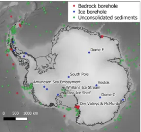
Fig. 1. Locations of compiled GHF estimates from temperature gradients 8. Data available from https://github.com/RicardaDziadek/Antarctic-GHF-DB.
Few GHF estimates have been made in Antarctica from bedrock boreholes, and none have been made from bedrock boreholes beneath the ice sheet (Fig.1). The temperature gradient of the uppermost 10-50 m of exposed crust is dominantly affected by downward conduction of the surface temperature rather than GHF. To address this, temperature measurements are made over the largest depth range possible. Shallow (<~10 m) temperature gradients for GHF estimation in unconsolidated sediments can be recorded using gravity-driven probes rather than boreholes. Measurements can be taken from unconsolidated sediments offshore 32,33, in subglacial lakes 25, or below ice shelves 34. As with borehole measurements, probe measurements must be from sufficient depth to represent the crustal temperature gradient and not be perturbed by temperature variation in the overlying water or ice 32. The GHF can be estimated from ice borehole temperature gradients if there is no additional heating from basal shear or horizontal advection, and if the ice sheet has been unequivocally in stationary contact with the bed long enough that the bedrock and basal ice are thermally equilibrated. GHF can be estimated from the englacial temperature via two methods: 1) if the borehole reaches the ice-bedrock interface then the GHF can be estimated using the temperature gradient in the ice near the interface 35; or 2) if a profile hasn’t been measured in the ice at the interface, the GHF can be varied in a thermal model until the measured basal temperature 36 or englacial temperature profile 37 is reproduced.
Thermal modelling is required to compensate for heat diffusion and equilibration with glacial-interglacial cycles.
4.2. Geophysical and geological methods to estimate GHF
Geophysical methods also derive GHF from temperature gradients by estimating the temperature within the lithosphere or mantle, and assuming that heat is vertically transferred by conduction 38. Magnetic data can estimate the depth to the bottom of the deepest magnetic sources within the lithosphere, assuming that this represents the depth at which the rocks exceed the maximum temperature of ferromagnetic magnetisation (the Curie isotherm of magnetite, 580 °C;
Fig. 2)39. Using this temperature at depth, and an assumed bedrock surface temperature, the GHF is estimated by solving the heat conduction equation considering the Curie depth and other boundary conditions as well as specific thermal parameters constrained based on local estimates, geology, and crustal architecture (Fig. 3a and 3b) 40–42. Generally, regions where the depth of the
Curie isotherm is shallower are thus expected to have higher temperature gradients and higher GHF than where it is deeper (excluding regions of exceptionally high HP at shallow crustal depths).
Fig. 2. Illustration of a convergent margin between oceanic and continental lithosphere to clarify the geological concepts and terms used in this paper.
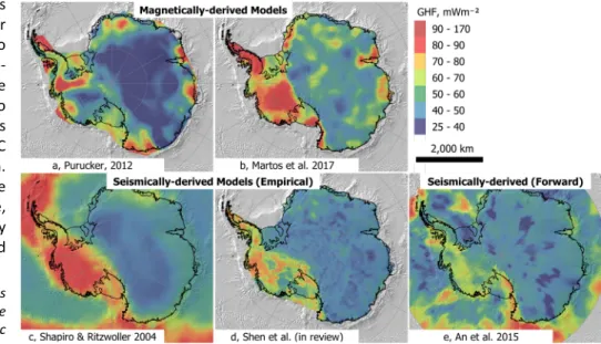
Temperature is the dominant control on mantle seismic velocity 43, enabling Antarctic GHF to be estimated from seismic data via: 1) empirical comparison of the lithospheric mantle and crustal seismic velocity models of Antarctica with other better-constrained regions (Fig. 3c and 3d) 44,45; or 2) forward modelling of the geological and thermal structures of the mantle and lithosphere (Fig 3e) 46. The empirical comparison approach is based on the observation that regions with similar shallow mantle seismic structures also share similar GHF estimates; a result of the thermal state controlling both variables. As an example, the resolution of the original empirical study on Antarctic GHF using global data (Fig. 3c) 44 has been improved using higher resolution data from North America 45 (Fig. 3d).
In forward modelling, changes in seismic velocity 46,47 or anisotropy 48 are used to identify the lithosphere- asthenosphere boundary (the change from a strong to ductile mantle, Fig. 2), which is associated with the ~1330°C
“mantle adiabat” isotherm.
Having estimated the thickness of the lithosphere, GHF can be estimated by assigning to it values of HP and thermal conductivity.
Fig. 3. Geophysical GHF estimates derived from magnetic Curie depth estimates 40,41 and seismic models 44–46.
Gravity data can also be used to estimate crustal and lithospheric thickness 49,50. Using the thickness estimates derived from seismology as constraints, models of the mantle and lithospheric structure are made by adjusting crustal density and crustal thickness until the observed variation in gravity and elevation is reproduced 49. By assigning values of HP and thermal conductivity to the models, surface heat flow can be estimated 49.
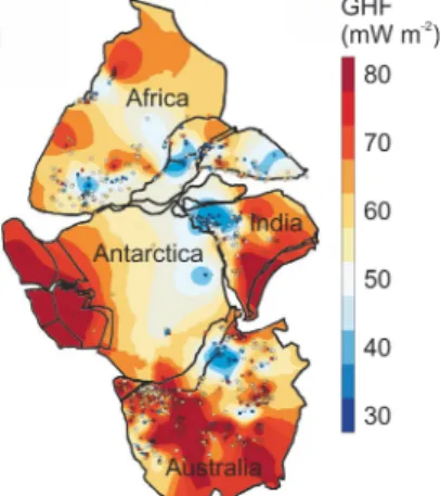
The GHF of East Antarctica can be estimated by reconstructing the pre-breakup Gondwanan supercontinent, and interpolating a GHF estimate through the borehole-derived point estimates (Fig. 4) 51. When extrapolating heat flow away from the margins into the interior of Antarctica, this approach is limited by the method of interpolation used and the quality and scarcity of the borehole-derived GHF estimates in the Antarctic interior. However, this Gondwanan synthesis approach is well suited to comparing in situ GHF estimates from formerly contiguous continents as a means to validate Antarctic GHF models.
The lithosphere’s thermal state contributes to its isostasy and surface elevation. By normalising the elevation of the continental lithosphere using an isostatic correction for crustal thickness and density, thermal isostasy can be investigated 52,53. This corrected elevation increases with increasing GHF, allowing GHF estimation. Application to Antarctica 54 provides an alternative GHF estimate based on two better-constrained variables: surface and bedrock topography. However, it is dependent on the quality of crustal thickness, density,
and HP estimates. Crust that has been tectonically or/and magmatically active in the Cenozoic may be thermally transient rather than steady-state 55,56 so this thermal isostasy approach is more applicable in East than West Antarctica.
All of these geophysical approaches assume that similar characteristics exist for tectonic provinces from different continents, including crustal HP, crustal and mantle conductivity, and the complex relationship between petrophysical parameters. Especially for the latter, constraints are needed from rock measurements.
Fig. 4. Interpolated Antarctic GHF using the reconstructed conjugate margins of the Gondwanan supercontinent. Terrestrial heat flow data shown by points. Adapted from Pollett et al. (2019) 51.
4.3. Calculation of GHF from measured heat production (HP) in rocks
Heat production is concentrated in the rocks of the upper crust. GHF can thus be empirically estimated 57,58 by taking the measured HP in rocks and assuming values for mantle heat flow, the reduced HP in the middle and lower crust, and the thickness of the upper crustal heat-producing layer. Using samples from exposed outcrops, this approach has been applied to transects near Prydz Bay 28,59 and extrapolated across the Antarctic Peninsula 60, demonstrating the impact geologically-controlled HPE heterogeneity in the upper crust has on total GHF. Similarly, glacially-transported rock samples from moraines of the Transantarctic Mountains were used to determine upstream HP of the unexposed East Antarctic crust 61. This indicated that the continental lithosphere beneath the East Antarctic ice sheet has comparable GHF to other Precambrian cratons elsewhere (i.e. >542 Ma tectonically-stable continental crust; e.g. central Canada).
Where xenoliths (rock fragments of the deep crust or mantle entrained in magma rising from depth) are available and of a suitable composition, their pressure and temperature dependent mineralogy can constrain the lithospheric geothermal gradient (Fig. 5) 17,62. This relies on a sufficient number of xenoliths from various depths 62. In Antarctica, geothermal gradients have been calculated using xenoliths from the Transantarctic Mountains, adjacent volcanic islands 56,63,64, and the margins of the Amery Ice Shelf 65. As well as constraining the geothermal gradient, HP, and conductivity of the unexposed lithosphere, xenoliths reflect the geothermal gradient when they were entrained by ascending lava, so can constrain the evolution of the geothermal gradient through time.
Fig. 5. Petrologically determined geotherms for East Antarctica (Amery Rift) 65 and West Antarctica (NVL: northern Victoria Land; SVL: southern Victoria Land) 64,66.
4.4.Glaciological inverse estimation of GHF
GHF can be estimated from our understanding of its effects on the overlying ice sheet via inverse modelling of observed glaciological properties (e.g. glacial flow and melt rates) and calculating the required GHF values.
The radar reflectivity of the ice-bedrock interface depends on the presence of water, so radar surveys can be used to map subglacial water. Glaciological modelling can then be used to estimate the minimum values of GHF required to elevate basal temperatures above the pressure melting point. Various approaches have estimated GHF from radar data, including: integrating water routing models to consider the melt distribution across the broader hydrological system 21; comparing the basal melt distribution with basal topography to derive the regional depth variation of the pressure melting point 67; and considering temperature-dependent dielectric loss through the ice column (radar attenuation is a strong function of the ice-sheet temperature profile) 68,69. Radar sounding profiles can also identify the drawdown of internal ice sheet layers caused by enhanced basal melting. By using this radar data and ages from ice cores to determine basal melt rates, and assuming the basal temperature is at the pressure melting point, thermal modelling can estimate the GHF required to reproduce the melt rate 70.
If temperatures are sufficient for basal melting, and topographic depressions are suitable, subglacial lakes can develop.
Subglacial lakes exhibit higher radio reflectivities than the ice-bedrock boundary, allowing the identification of 402 Antarctic subglacial lakes to date 71,72. When lakes are located near ice divides, heat from horizontal advection, basal friction, and internal deformation is minimal. Thus, the heat required to bring the basal ice above the pressure melting point is a product of ice thickness and GHF, and minimum GHF point estimates can be calculated from thermal models.
This assumes that water was derived locally and not routed from elsewhere, as lakes only form in topographic depressions. The absence of a lake or basal water does not imply a frozen bed if water can drain away 73,74.
Englacial temperature profiles (from which GHF can be estimated) can be derived from satellite and airborne passive detection of microwave radiation (~1.4 GHz 75–77). These wavelengths have very low absorption and scattering in ice, providing high penetration depths. The corrected microwave intensity (TB) correlates with ice surface temperature, but is also affected by ice sheet thickness, density profile, and grain size. Thus, the ice sheet’s thermal structure at depth can be estimated by comparing the observed TB with a simulated TB from microwave emissivity modelling. Deriving englacial temperature from microwave emissivity is optimal in areas of very slow flowing ice (<5 m yr-1), where heating by horizontal advection or ice deformation is minimal, and where ice is >1 km thick; the conditions where GHF has the greatest influence on ice sheet dynamics. However, this method is not strongly sensitive to the englacial temperature profile below 1-1.5 km. Longer wavelengths (0.5 GHz) with greater sensitivity to the deeper temperature profile may provide the increased accuracy at depth necessary for accurate GHF estimation 78.
5. Current challenges
5.1. Borehole and probe-derived estimates
A fundamental limitation for Antarctic GHF estimation is the lack of borehole-derived estimates beneath the Antarctic ice sheet. Without these validation points, regional estimates cannot be accurately evaluated. The most promising future development will be the ≥25 m deep bedrock borehole measurements of the Rapid Access Ice Drill project RAID
79. However, as noted above, local temperature gradients may not be representative of the regional heat flow, as local geology, hydrothermal circulation, and topography can result in localised GHF variability. In response, multiple boreholes are required to categorise the regional variation and topographic effects must be accounted for.
Beyond bedrock drilling much can be gained from further ice boreholes. Existing data must be evaluated to ensure that the methodologies of GHF modelling from borehole temperature profiles are consistent and accurate 80. Future ice boreholes into stationary ice, frozen to the bed, have the potential to supplement the existing borehole and probe- derived GHF estimates, particularly if the proposed methodology for determining GHF from shallow boreholes can be validated (600 m depth, or the upper 20% of the ice column) 81–83.
5.2.Geophysical GHF estimates
Whilst only geophysical methods have provided continent-scale GHF estimates, the resulting values and distribution of GHF vary greatly (Fig. 3 and Fig. 6); although all estimates note the clear difference between East and West Antarctica.
The largest limitations are uncertainties in the structure, composition, HP, and thermophysical properties of the unexposed crust, lithosphere, and underlying mantle. Most models assume the lithosphere to be laterally homogenous in composition and thermophysical properties, despite studies on the effects of variable upper crustal HP.
The estimates also assume that lithospheric HP either exponentially decreases with depth 40,41 or is concentrated in an uppermost layer of constant HP 46,84. However, deep boreholes and crustal sections show that whilst HP correlates with lithology, there is no such correlation with depth or metamorphic grade 85–88.
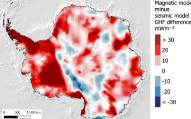
Fig. 6. Difference in heat flow values between the most recent magnetic
41 and seismic 46 heat flow models.
Consistent 3D lithospheric structure models for Antarctica may reduce the uncertainty in the GHF contribution from the unexposed crust and deeper lithosphere. Such models can be derived by integrating seismic, magnetic, and thermal-isostatic data, and assigning values of HP, conductivity, and petrophysical properties (from exposed lithologies, xenoliths, and crustal sections) to estimate GHF. A similar model was developed for Norway 89,90, providing a framework that would build upon recent 2D and 3D geophysically-derived Antarctic models 49,50,91. Where the bedrock is obscured, HP is best constrained from glacially-eroded and transported clasts 61. The assumption of a homogenous mantle beneath East Antarctica is challenged by discrepancies in the Moho depth estimates derived by gravity, seismic, and isostatic modelling 49,50,92, as this indicates variable mantle densities. A review of mantle-derived samples may constrain the mantle composition, and thermal-isostatic modelling may identify anomalous regions 84. Stochastic analysis shows that models based on different geophysical techniques are partially incompatible and that using incorrect models or sparsely available data leads to unreliable results 93. Therefore, approaches that systematically explore data quality and coverage are needed to provide uncertainties to any estimates. For example, a global terrestrial GHF map was developed from empirical correlation of measurements with geophysical and geological data sets 18. Similarly, machine learning was used to predict GHF in Greenland 94. While the advantage of these approaches is that many possible geophysical and geological models can be explored, a challenge is the often (at least in a global comparison) low accuracy of such models for Antarctica. Therefore, increased efforts must target improved data sets, models and approaches. ADMAP-2 95 or BedMachine Antarctica 96 are examples of high-quality data sets that can be used for such statistical analysis.
5.3. Glaciological GHF estimates
Englacial temperatures are more sensitive to GHF in the Antarctic interior where basal sliding is negligible. Of the methods discussed here, the most promising is englacial temperature estimation from microwave emission at a longer wavelength (0.5 GHz) than currently available (~1.4 GHz). The longer wavelength will reduce uncertainty in the ice temperature at >1 km depth 78, reducing the extrapolation of the deeper englacial temperature gradient required for inverse glaciological modelling of GHF. This requires the acquisition of new satellite or airborne data, as advocated by the unsuccessful 2018 Cryorad ESA proposal 97.
A challenge for radar-derived subglacial water distribution is our ability to discriminate between water at the bed and other sources of enhanced reflectivity (e.g. the geometry of the basal interface) 21. Improved radar techniques, particularly those considering temperature-dependent radar attenuation 68,69 and englacial layers, combined with seismic surveys and direct access observations will improve our estimates of englacial temperatures, melt rates, and subglacial hydrology 98.
Finally, the glaciological models used to infer GHF must be improved. The thermal models used to infer GHF can be classified into three groups: 1) 1D time-dependent high-complexity models; 2) 2D/3D steady-state low-complexity models; and 3) ice sheet evolution models, where the full thermomechanical field is calculated and long simulations can take into account glacial-interglacial temperature changes. The first are generally used near ice domes or ridges with low horizontal flow, where horizontal heat advection can be neglected 67. The second are used across the continent 22, but ignore changes in temperature between glacial and interglacial periods; despite their strong effect on englacial temperatures 99. The third are too computer intensive to be used in inverse modelling, and are instead used for forward modelling of ice sheet geometry with time. However, these forward models do not provide a perfect fit between observed and simulated geometry for the present time. The challenge is to develop operational thermal models with the required complexity at a continental scale, accommodating the main physical processes.
6. Aspirations and deliverables
Within the new SCAR Scientific Research Programmes, the international GHF community will reconcile the differences between GHF estimates and produce regional and continental-scale estimates of quantified accuracy. Regions where ice dynamics are highly sensitive to GHF will be targeted, and the uncertainty and limitations of future models communicated clearly to the broader scientific community. Our ultimate aim is to generate a validated, spatially- accurate and high-resolution Antarctic GHF distribution based on quantifiable, variable uncertainty. This will require a multi-disciplinary effort to derive, validate, and communicate our results across the Antarctic research community.
7. Recommended future directions
- Estimate local GHF from the thermal gradient in subglacial bedrock boreholes (e.g. RAID) 79.
- Validate the feasibility for GHF estimation from shallow glacial boreholes, using new and existing borehole data to expand local GHF estimates 81–83.
- Collect long-wavelength microwave emissivity data via satellite, airborne, and ground-based sensors 97. - Consider topographic effects in GHF estimates at all scales.
- Support the development of radar sounding systems and analyses optimised for constraining englacial and basal temperatures.
- Use evidence for basal melting to improve and expand inverse glaciological GHF estimates 21,67,68,100.
- Improve the thermal models used for inverse glaciological modelling, developing continental models that accurately incorporate the variation and effects of temperature between glacial and interglacial periods 99.
- Collate available radar reflectivity data for the identification of basal melting, englacial layers, and englacial temperature-dependent radar attenuation (e.g. via the SCAR “AntArchitecture” Action Group, collating the data on Antarctic internal layering 101).
- Derive new, enhanced geophysically-derived GHF estimates by combining seismic, magnetic, gravity and thermal isostasy models to constrain the three-dimensional structure and composition of the mantle and lithosphere 49,50,89,90. - Expand the database of crustal geochemistry determined from rock outcrops and glacial deposits.
- Validate GHF models against geology, using xenoliths, crustal sections, and areas of well-exposed outcrop.
- Support better resolved 3D models of the Antarctic mantle using integrated geophysical and remote sensing techniques, and geological information from outcrop and mantle xenoliths.
- Integrate into the geophysical approaches a more accurate model of the structure and distribution of heat producing elements within the crust 89–91, considering heterogeneities in the underlying mantle.
- Statistical exploitation of the existing data sets to provide predictions and uncertainties.
- Ensure future GHF estimates and uncertainties are accurately and transparently communicated to the broader scientific community, particularly ice sheet modellers, hosting estimates and models on an accessible platform (e.g.
Quantarctica 102).
- Continue to support international interdisciplinary communication and data access via SCAR (as has been achieved via the SERCE GHF sub-group).
8. References
1. Larour, E., Morlighem, M., Seroussi, H., Schiermeier, J. & Rignot, E. Ice flow sensitivity to geothermal heat flux of Pine Island Glacier, Antarctica. Journal of Geophysical Research: Earth Surface 117, (2012).
2. Llubes, M., Lanseau, C. & Rémy, F. Relations between basal condition, subglacial hydrological networks and geothermal flux in Antarctica. Earth and Planetary Science Letters 241, 655–662 (2006).
3. Greve, R. & Hutter, K. Polythermal three-dimensional modelling of the Greenland ice sheet with varied geothermal heat flux.
Annals of Glaciology 21, 8–12 (1995).
4. Siegert, M. J. Antarctic subglacial lakes. Earth-Science Reviews 50, 29–50 (2000).
5. Winsborrow, M. C., Clark, C. D. & Stokes, C. R. What controls the location of ice streams? Earth-Science Reviews 103, 45–59 (2010).
6. Burton-Johnson, A., Dziadek, R. & Shen, W. Report of the Geothermal Heat Flux Side Meeting at XIII ISAES, 2019. 7 https://www.scar.org/scar-library/search/science-4/research-programmes/serce/5334-ghf-meeting-report-2019/file (2019).
7. Halpin, J. A. & Reading, A. M. Report on Taking the Temperature of the Antarctic Continent (TACtical) Workshop 21-23 March 2018, Hobart, Tasmania, Australia. 3 (2018).
8. Burton-Johnson, A., Dziadek, R. & Martin, C. Geothermal heat flow in Antarctica: current and future directions. The Cryosphere Discussions (2020) doi:https://doi.org/10.5194/tc-2020-59.
9. Reading, A. M. et al. Antarctic Geothermal Heat Flow. Nature Reviews: Earth & Environment (in prep.).
10. Gutenberg, B. 6. Temperature and Thermal Processes in the Earth. in International Geophysics (ed. Gutenberg, B.) vol. 1 121–
148 (Academic Press Inc., 1959).
11. Pollack, H. N., Hurter, S. J. & Johnson, J. R. Heat flow from the Earth’s interior: Analysis of the global data set. Reviews of Geophysics 31, 267–280 (1993).
12. Beardsmore, G. R. & Cull, J. P. Crustal heat flow: a guide to measurement and modelling. (Cambridge University Press, 2001).
13. Lowrie, W. Fundamentals of geophysics. (Cambridge University Press, 2007). doi:10.1017/CBO9780511807107.
14. Boden, D. R. Geology and Heat Architecture of the Earth’s Interior. in Geologic Fundamentals of Geothermal Energy (Routledge, 2016). doi:10.1201/9781315371436-4.
15. McDonough, W. F. & Sun, S. s. The composition of the Earth. Chemical Geology 120, 223–253 (1995).
16. Nyblade, A. A. & Pollack, H. N. A comparative study of parameterized and full thermal-convection models in the interpretation of heat flow from cratons and mobile belts. Geophysical Journal International 113, 747–751 (1993).
17. Goes, S., Govers, R., Vacher & P. Shallow mantle temperatures under Europe from P and S wave tomography. Journal of Geophysical Research: Solid Earth 105, 11153–11169 (2000).
18. Lucazeau, F. Analysis and mapping of an updated terrestrial heat flow dataset. Geochemistry, Geophysics, Geosystems 20, 4001–4024 (2019).
19. Mareschal, J. C. & Jaupart, C. Radiogenic heat production, thermal regime and evolution of continental crust. Tectonophysics 609, 524–534 (2013).
20. Pollard, D., DeConto, R. M. & Nyblade, A. A. Sensitivity of Cenozoic Antarctic ice sheet variations to geothermal heat flux. Global and Planetary Change 49, 63–74 (2005).
21. Schroeder, D. M., Blankenship, D. D., Young, D. A. & Quartini, E. Evidence for elevated and spatially variable geothermal flux beneath the West Antarctic Ice Sheet. Proceedings of the National Academy of Sciences 111, 9070–9072 (2014).
22. Van Liefferinge, B. et al. Promising Oldest Ice sites in East Antarctica based on thermodynamical modelling. The Cryosphere 12, 2773–2787 (2018).
23. van der Wal, W., Whitehouse, P. L. & Schrama, E. J. Effect of GIA models with 3D composite mantle viscosity on GRACE mass balance estimates for Antarctica. Earth and Planetary Science Letters 414, 134–143 (2015).
24. van der Wal, W. et al. Glacial isostatic adjustment model with composite 3-D Earth rheology for Fennoscandia. Geophysical Journal International 194, 61–77 (2013).
25. Fisher, A. T. et al. High geothermal heat flux measured below the West Antarctic Ice Sheet. Science advances 1, e1500093 (2015).
26. Bullard, E. C. The disturbance of the temperature gradient in the earth’s crust by inequalities of height. Geophysical Supplements to the Monthly Notices of the Royal Astronomical Society 4, 360–362 (1938).
27. Lees, C. H. On the shapes of the isogeotherms under mountain ranges in radio-active districts. Proceedings of the Royal Society of London. Series A, Containing Papers of a Mathematical and Physical Character 83, 339–346 (1910).
28. Carson, C. J., McLaren, S., Roberts, J. L., Boger, S. D. & Blankenship, D. D. Hot rocks in a cold place: high sub-glacial heat flow in East Antarctica. Journal of the Geological Society 171, 9–12 (2014).
29. Hasterok, D. & Chapman, D. S. Heat production and geotherms for the continental lithosphere. Earth and Planetary Science Letters 307, 59–70 (2011).
30. Fisher, A. T. & Harris, R. N. Using seafloor heat flow as a tracer to map subseafloor fluid flow in the ocean crust. Geofluids 10, 142–160 (2010).
31. Bachu, S. Analysis of heat transfer processes and geothermal pattern in the Alberta Basin, Canada. Journal of Geophysical Research: Solid Earth 93, 7767–7781 (1988).
32. Dziadek, R., Gohl, K. & Kaul, N. Elevated geothermal surface heat flow in the Amundsen Sea Embayment, West Antarctica. Earth and Planetary Science Letters 506, 530–539 (2019).
33. Dziadek, R., Gohl, K., Diehl, A. & Kaul, N. Geothermal heat flux in the Amundsen Sea sector of West Antarctica: New insights from temperature measurements, depth to the bottom of the magnetic source estimation, and thermal modeling.
Geochemistry, Geophysics, Geosystems 18, 2657–2672 (2017).
34. Begeman, C. B., Tulaczyk, S. M. & Fisher, A. T. Spatially variable geothermal heat flux in West Antarctica: evidence and implications. Geophysical Research Letters 44, 9823–9832 (2017).
35. Engelhardt, H. Ice temperature and high geothermal flux at Siple Dome, West Antarctica, from borehole measurements. Journal of Glaciology 50, 251–256 (2004).
36. Fudge, T. J., Biyani, S., Clemens-Sewall, D. & Hawley, B. Constraining geothermal flux at coastal domes of the Ross Ice Sheet, Antarctica. Geophysical Research Letters 46, 13090–13098 (2019).
37. Zagorodnov, V. et al. Borehole temperatures reveal details of 20th century warming at Bruce Plateau, Antarctic Peninsula. The Cryosphere 6, 675–686 (2012).
38. Turcotte, D. L. & Schubert, G. Geodynamics. (Cambridge University Press, 2014).
39. Haggerty, S. E. Mineralogical contraints on Curie isotherms in deep crustal magnetic anomalies. Geophysical Research Letters 5, 105–108 (1978).
40. Purucker, M. Geothermal heat flux data set based on low resolution observations collected by the CHAMP satellite between 2000 and 2010, and produced from the MF-6 model following the technique described in Fox Maule et al. (2005), available at: http://websrv.cs.umt.edu/isis/images/c/c8/Antarctica_heat_flux_5km.nc. (2012).
41. Martos, Y. M. et al. Heat flux distribution of Antarctica unveiled. Geophysical Research Letters 44, 11–417 (2017).
42. Martos, Y. M., Catalan, M. & Galindo-Zaldivar, J. Curie Depth, Heat Flux, and Thermal Subsidence Reveal the Pacific Mantle Outflow Through the Scotia Sea. Journal of Geophysical Research: Solid Earth 124, 10735–10751 (2019).
43. Carlson, R. W., Pearson, D. G. & James, D. E. Physical, chemical and chronological characteristics of continental mantle. Reviews in Geophysics 43, RG1001 (2005).
44. Shapiro, N. M. & Ritzwoller, M. H. Inferring surface heat flux distributions guided by a global seismic model: particular application to Antarctica. Earth and Planetary Science Letters 223, 213–224 (2004).
45. Shen, W., Wiens, D. A., Lloyd, A. & Nyblade, A. A Geothermal heat flux map of Antarctica empirically constrained by seismic structure. Geophysical Research Letters (In review).
46. An, M. et al. Temperature, lithosphere-asthenosphere boundary, and heat flux beneath the Antarctic Plate inferred from seismic velocities. Journal of Geophysical Research: Solid Earth 120, 8720–8742 (2015).
47. An, M. et al. S-velocity model and inferred Moho topography beneath the Antarctic Plate from Rayleigh waves. Journal of Geophysical Research: Solid Earth 120, 359–383 (2015).
48. Eaton, D. W. et al. The elusive lithosphere–asthenosphere boundary (LAB) beneath cratons. Lithos 109, 1–22 (2009).
49. Pappa, F., Ebbing, J. & Ferraccioli, F. Moho Depths of Antarctica: Comparison of Seismic, Gravity, and Isostatic Results.
Geochemistry, Geophysics, Geosystems 20, 1629–1645 (2019).
50. Pappa, F., Ebbing, J., Ferraccioli, F. & van der Wal, W. Modeling satellite gravity gradient data to derive density, temperature, and viscosity structure of the Antarctic lithosphere. Journal of Geophysical Research: Solid Earth 124, 12053–12076 (2019).
51. Pollett, A. et al. Heat flow in southern Australia and connections with East Antarctica. Geochemistry, Geophysics, Geosystems 20, 5352–5370 (2019).
52. Hasterok, D. & Chapman, D. S. Continental thermal isostasy: 1. Methods and sensitivity. Journal of Geophysical Research: Solid Earth 112, (2007).
53. Hasterok, D. & Chapman, D. S. Continental thermal isostasy: 2. Application to North America. Journal of Geophysical Research:
Solid Earth 112, (2007).
54. Hasterok, D. P. et al. Constraining Geothermal Heat Flux Beneath Ice Sheets Using Thermal Isostasy. in AGU Fall Meeting 2019 (AGU, 2019).
55. Wörner, G. & Zipfel, J. A mantle PT path for the Ross Sea rift margin, Antarctica, derived from mineral zoning in peridotite xenoliths. Geologisches Jahrbuch Reihe B 157–168 (1996).
56. Martin, A. P., Cooper, A. F. & Price, R. C. Increased mantle heat flow with on-going rifting of the West Antarctic rift system inferred from characterisation of plagioclase peridotite in the shallow Antarctic mantle. Lithos 190, 173–190 (2014).
57. Lachenbruch, A. H. Preliminary geothermal model of the Sierra Nevada. Journal of Geophysical Research 73, 6977–6989 (1968).
58. Roy, R. F., Blackwell, D. D. & Birch, F. Heat generation of plutonic rocks and continental heat flow provinces. Earth and Planetary Science Letters 5, 1–12 (1968).
59. Carson, C. J. & Pittard, M. A Reconaissance Crustal Heat Production Assessment of the Australian Antarctic Territory (AAT).
(2012).
60. Burton-Johnson, A., Halpin, J. A., Whittaker, J. M., Graham, F. S. & Watson, S. J. A new heat flux model for the Antarctic Peninsula incorporating spatially variable upper crustal radiogenic heat production. Geophysical Research Letters 44, 5436–5446 (2017).
61. Goodge, J. W. Crustal heat production and estimate of terrestrial heat flow in central East Antarctica, with implications for thermal input to the East Antarctic ice sheet. Cryosphere 12, 491–504 (2018).
62. O’Reilly, S. Y., Jackson, I. & Bezant, C. Equilibration temperatures and elastic wave velocities for upper mantle rocks from eastern Australia: implications for the interpretation of seismological models. Tectonophysics 185, 67–82 (1990).
63. Berg, J. H., Moscati, R. J. & Herz, D. L. A petrologic geotherm from a continental rift in Antarctica. Earth and Planetary Science Letters 93, 98–108 (1989).
64. Perinelli, C., Armienti, P. & Dallai, L. Geochemical and O-isotope constraints on the evolution of lithospheric mantle in the Ross Sea rift area (Antarctica). Contributions to Mineralogy and Petrology 151, 245–266 (2006).
65. Foley, S. F., Andronikov, A. V., Jacob, D. E. & Melzer, S. Evidence from Antarctic mantle peridotite xenoliths for changes in mineralogy, geochemistry and geothermal gradients beneath a developing rift. Geochimica et Cosmochimica Acta 70, 3096–
3120 (2006).
66. Martin, A. P., Price, R. C., Cooper, A. F. & McCammon, C. A. Petrogenesis of the rifted southern Victoria Land lithospheric mantle, Antarctica, inferred from petrography, geochemistry, thermobarometry and oxybarometry of peridotite and pyroxenite xenoliths from the Mount Morning eruptive centre. Journal of Petrology 56, 193–226 (2015).
67. Passalacqua, O., Ritz, C., Parrenin, F., Urbini, S. & Frezzotti, M. Geothermal flux and basal melt rate in the Dome C region inferred from radar reflectivity and heat modelling. The Cryosphere 11, 2231–2246 (2017).
68. Carter, S. P., Blankenship, D. D., Young, D. A. & Holt, J. W. Using radar-sounding data to identify the distribution and sources of subglacial water: application to Dome C, East Antarctica. Journal of Glaciology 55, 1025–1040 (2009).
69. Schroeder, D. M., Seroussi, H., Chu, W. & Young, D. A. Adaptively constraining radar attenuation and temperature across the Thwaites Glacier catchment using bed echoes. Journal of Glaciology 62, 1075–1082 (2016).
70. Jordan, T. A. et al. Anomalously high geothermal flux near the South Pole. Scientific reports 8, 16785 (2018).
71. Siegert, M. J., Ross, N. & Le Brocq, A. M. Recent advances in understanding Antarctic subglacial lakes and hydrology.
Philosophical Transactions of the Royal Society A: Mathematical, Physical and Engineering Sciences 374, 20140306 (2016).
72. Siegert, M. J., Carter, S., Tabacco, I., Popov, S. & Blankenship, D. D. A revised inventory of Antarctic subglacial lakes. Antarctic Science 17, 453–460 (2005).
73. Pattyn, F. Antarctic subglacial conditions inferred from a hybrid ice sheet/ice stream model. Earth and Planetary Science Letters 295, 451–461 (2010).
74. Siegert, M. J. & Dowdeswell, J. A. Spatial variations in heat at the base of the Antarctic ice sheet from analysis of the thermal regime above subglacial lakes. Journal of Glaciology 42, 501–509 (1996).
75. Macelloni, G. et al. On the retrieval of internal temperature of Antarctica Ice Sheet by using SMOS observations. Remote Sensing of Environment 233, 111405 (2019).
76. Macelloni, G., Leduc-Leballeur, M., Brogioni, M., Ritz, C. & Picard, G. Analyzing and modeling the SMOS spatial variations in the East Antarctic Plateau. Remote sensing of environment 180, 193–204 (2016).
77. Passalacqua, O. et al. Retrieval of the Absorption Coefficient of L-Band Radiation in Antarctica From SMOS Observations.
Remote Sensing 10, 1954 (2018).
78. Jezek, K. C. et al. Radiometric approach for estimating relative changes in intraglacier average temperature. IEEE Transactions on Geoscience and Remote Sensing 53, 134–143 (2014).
79. Goodge, J. W. & Severinghaus, J. P. Rapid Access Ice Drill: a new tool for exploration of the deep Antarctic ice sheets and subglacial geology. Journal of Glaciology 62, 1049–1064 (2016).
80. Mony, L., Roberts, J. L. & Halpin, J. A. Inferring geothermal heat flux from an ice-borehole temperature profile at Law Dome, East Antarctica. Journal of Glaciology 1–11.
81. Hindmarsh, R. C. & Ritz, C. M. How deep do you need to drill through ice to measure the geothermal heat flux? in EGU General Assembly Conference Abstracts vol. 14 8629 (2012).
82. Mulvaney, R., Martin, C., Massam, A., Rix, J. & Ritz, C. Estimating geothermal heat flux from ice sheet borehole temperature measurements. in XIII International Symosium on Antarctic Earth Sciences (2019).
83. Rix, J., Mulvaney, R., Hong, J. & Ashurst, D. Development of the British Antarctic Survey Rapid Access Isotope Drill. Journal of Glaciology 65, 288–298 (2019).
84. Hasterok, D. & Gard, M. Utilizing thermal isostasy to estimate sub-lithospheric heat flow and anomalous crustal radioactivity.
Earth and Planetary Science Letters 450, 197–207 (2016).
85. Alessio, K. L. et al. Conservation of deep crustal heat production. Geology 46, 335–338 (2018).
86. Veikkolainen, T. & Kukkonen, I. T. Highly varying radiogenic heat production in Finland, Fennoscandian Shield. Tectonophysics 750, 93–116 (2019).
87. Bea, F. The sources of energy for crustal melting and the geochemistry of heat-producing elements. Lithos 153, 278–291 (2012).
88. Bea, F. & Montero, P. Behavior of accessory phases and redistribution of Zr, REE, Y, Th, and U during metamorphism and partial melting of metapelites in the lower crust: an example from the Kinzigite Formation of Ivrea-Verbano, NW Italy. Geochimica et Cosmochimica Acta 63, 1133–1153 (1999).
89. Ebbing, J., Lundin, E., Olesen, O. & Hansen, E. K. The mid-Norwegian margin: a discussion of crustal lineaments, mafic intrusions, and remnants of the Caledonian root by 3D density modelling and structural interpretation. Journal of the Geological Society 163, 47–59 (2006).
90. Olesen, O. et al. KONTIKI final report, continental crust and heat generation in 3D. NGU Report 42, (2007).
91. Leat, P. T. et al. Jurassic high heat production granites associated with the Weddell Sea rift system, Antarctica. Tectonophysics 722, 249–264 (2018).
92. Stål, T., Reading, A. M., Halpin, J. A. & Whittaker, J. M. A multivariate approach for mapping lithospheric domain boundaries in East Antarctica. Geophysical Research Letters 46, 10404–10416 (2019).
93. Lösing, M., Ebbing, J. & Szwillus, W. Geothermal Heat Flux in Antarctica: Assessing Models and Observations by Bayesian Inversion. Frontiers in Earth Science 8, 105 (2020).
94. Rezvanbehbahani, S., Stearns, L. A., Kadivar, A., Walker, J. D. & van der Veen, C. J. Predicting the geothermal heat flux in Greenland: A machine learning approach. Geophysical Research Letters 44, 12–271 (2017).
95. Golynsky, A. V. et al. New Magnetic Anomaly Map of the Antarctic. Geophysical Research Letters 45, 6437–6449 (2018).
96. Morlighem, M. et al. Deep glacial troughs and stabilizing ridges unveiled beneath the margins of the Antarctic ice sheet. Nature Geoscience 13, 132–137 (2020).
97. Macelloni, G. et al. Cryorad: A Low Frequency Wideband Radiometer Mission for the Study of the Cryosphere. in IGARSS 2018- 2018 IEEE International Geoscience and Remote Sensing Symposium 1998–2000 (IEEE, 2018).
98. Ashmore, D. W. & Bingham, R. G. Antarctic subglacial hydrology: current knowledge and future challenges. Antarctic Science 26, 758–773 (2014).
99. Ritz, C. Interpretation of the temperature profile measured at Vostok, East Antarctica. Annals of glaciology 12, 138–144 (1989).
100. Jordan, T. et al. Newly discovered geothermal anomaly at South Pole ice divide; origins and implications. in Geophysical Research Abstracts vol. 20 15511 (2018).
101. AntArchitecture Action Group. AntArchitecture: Archiving and interrogating Antarctica’s internal structure from radar sounding. Final Report. in Workshop to establish scientific goals, working practices and funding routes. University of Edinburgh, UK (2017).
102. Matsuoka, K., Skoglund, A. & Roth, G. Quantarctica [Data set]. Norwegian Polar Institute (2018).