Solare Einstrahlung auf der Erde

(1)

Solare Einstrahlung auf der Erde

3.2

3.21 The revolution of the earth around the sun

Exkursionen: Veränderung der Bahnparameter in Jahrtausenden

Die Leuchtkraft der Sonne: kurzzeitige Schwankungen und astronomischer Trend

3.22 Solare Einstrahlung

.221 Wo steht die Sonne

_1 Zeitgleichung, _2 Azimut und Sonnenhöhe ._3 Direkte solare Inzidenz auf geneigte Fläche

.

222 Streuung und Absorption der Solarstrahlung

_1 Angström‘s turbidity _2 Linke‘s Trübungsfaktor _3 Parametrisierung [Kasten 95]

.

223 Diffuse und direkte Solarstrahlung

_0 Strahlungsgrößen (Überblick und Bezeichnung)

_1 Anteil der diffusen Strahlung an der Globalstrahlung /Reindl e.a.1990/

_2 Perez-Modell: die anisotrope Himmelsstrahlung /Perez e.a. 1990/

_3 Solar Tracking (Nachführung des Kollektors)

[.

224 Verschattung und Bodenreflektion]

3.23 Maps of horizontal surface global radiation

Welt, Europa, Deutschland, Saarheimat

3.24 Simulationsprogramme

.241 Excelblatt: Modellierung des Sonnenenergie -Dargebotes

.242 kommerzielle Simulationsprogramme

(hübsch, vermutlich korrekt, aber undurchsichtig und für Außergewöhnliches nicht zu gebrauchen)

(2)

Solar Astronomy

3.21

(3)

Unsere Sonne

(4)

To explain the sun‘s apparent motion about an observer on earth, we need to study both:

1. The revolution of the earth around the sun

2. The rotation of the earth on ist axis

(5)

Quelle:/ Wieder82, fig 2.1; p.20/

The earth‘s orbit

(shown with an exaggerated eccentricity )

the mean orbital distance is a = 149,7 [Gm] = 149,7 Mio km and the eccentricity is  = 0.0167

also ca. :: r = a +- 2%

cos  = -1  =0 ; cos  =+ 1

r

_a

= r

_Aphelion

=a (1+  ) r

_p

= r

_Perihelion

=a (1-  )

(6)

BQuelle: Strahler: „Physical Geography“,2002, Wiley-Verlag, ISBN=0-471-23800-7, Bild3.15,p.55

The tilt of

the Earth‘s axis

with respect to

its orbital plane

(ecliptic)

(7)

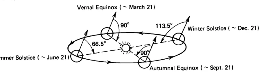
Fig 2.2: The seasonal variation of the angle between the earth 's polar axis and the

earth-sun line.

The angle of inclination

(between the earth axis of rotation and the line perpendicular to the ecliptic plane)

is 23.5° and remains constant throughout the year.

The rate of rotation is also constant and equal to one rotation every 23.93 hr = a sideral day.. Summer solstice (June 21) : earth axis of rotation is tilted 90 - 23,5 = 66.5 ° toward the sun

Winter solstice (December 21) : 90 + 23.5 = 113.5° away from the sun Autumnal equinox (September 23) : 90 °

Vernal equinox (March 21) : 90°

Seasons are a consequence of the inclination of the earth 's axis of rotation

(8)

BQuelle: Strahler: „Physical Geography“,2002, Wiley-Verlag, ISBN=0-471-23800-7, Bild3.16,p.55 bzw. G4e_01_17, (ein Buch mit wunderschönen Bildern)

The 4 seasons

(9)

Equinox

at equinox, the circle of

illumination

passes through both poles

the subsolar point is the equator

each location on Earth

experiences 12 hours of sunlight and 12 hours of darkness

BQuelle: Strahler: „Physical Geography“,2002, Wiley-Verlag, ISBN=0-471-23800-7, Bild3.17,p.56 (bzw. Fig.1.18,p.41 in neuerer Auflage)

(10)

Solstice

Solstice (“sun stands still”)

On June 22, the subsolar point is 23½°N (Tropic of Cancer) On Dec. 22, the subsolar point is 23½°S (Tropic of Capricorn)

BQuelle: Strahler: „Physical Geography“,2002, Wiley-Verlag, ISBN=0-471-23800-7, Bild3.18,p.56 (bzw. Fig.1.19,p.41 in neuerer Auflage)

(11)

Declination over the year

the latitude of the

subsolar point marks the

sun’s

declination which

changes throughout the

year

Figure 1.20, p. 42

BQuelle: Strahler: „Physical Geography“,2002, Wiley-Verlag, ISBN=0-471-23800-7, Bild3.16,p.55 [bzw. Fig.1.20,p42 ] (ein Buch mit wunderschönen Bildern)

(12)

(13)

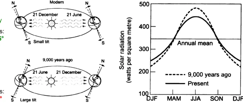
Fig. 5.19: Changes in the Earth's elliptical orbit from the present configuration to 9,000 years ago.(left) Changes in the average solar radiation during the year over the northern hemisphere (right).

The incoming solar energy averaged over the northern hemisphere was ca. 7 % greater in July and correspondingly less in January.

Urquelle:J.E. Kutzbach in „Climate System Modelling“ (1992). Quelle:/ Houghton, J.: „ Global Warming“ (1997), fig 5.19; p.82/

Today:

Perihelion in January Tilt of the earth‘s axis:

23.5°

9000 years ago::

Perihelion in July Tilt of the earth‘s axis:

24.0°

Configuration of the earth‘s orbit 9000 years ago

3.21a Exkursion

(14)

9000 years ago::

Perihelion in July rather than in January as it is now.

Tilt of the earth‘s axis 24.0°

The incoming solar energy averaged over the northern hemisphere was ca. 7 % greater in July and correspondingly less in January.

A different climate for these altered parameters

Model gives a different climate :

When these altered parameters are incorporated into a model a different climate results.

For instance:

• Northem continents are warmer in summer and colder in winter.

• In summer a significantly expanded low pressure region develops over north Africa and south Asia because of the increased land-ocean temperature contrast.

• The summer monsoons in these regions are strengthened and there is increased rainfall.

..in qualitative agreement with paleoclimatic data.

These simulated changes are in qualitative agreement with paleoclimate data.

For example:

• Evidence for lakes and vegetation in the southern Sahara about 1000 km north of the present limits of

vegetation.

Urquelle:J.E. Kutzbach in „Climate System Modelling“ (1992). Quelle:/ Houghton, J.: „ Global Warming“ (1997), fig 5.19; p.82/

(15)

Exkursion

Die Leuchtkraft der Sonne:

kurzzeitige Schwankungen und astronomischer Trend

3.21b

(16)

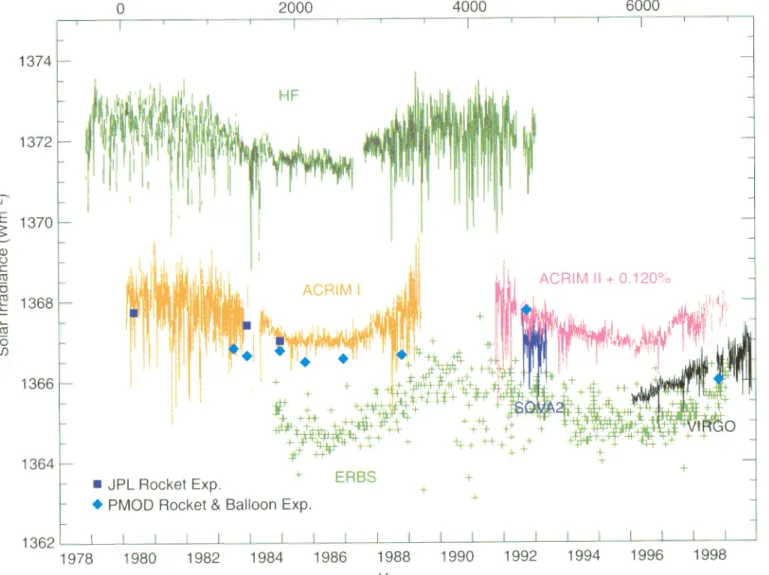
Figure 6.4:

Measurements of TSI made between 1979 and 1999 by satellite, rocket and balloon instruments

::

It is only since the late 1970s, however,

and the advent of space-borne measurements of total solar irradiance (TSI), that it has been clear that the solar “constant” does, in fact, vary.

These satellite instruments suggest a variation in annual mean TSI of the order 0.08%

(or about 1.1 Wm

^-2

) between minimum and maximum of the 11-year solar cycle.

Quelle: IPCC 2001: TAR1 The scientific basis, chap 6.11 , p.380ff /

Variations of the solar „constant“

Measurement uncertainties:

•The absolute calibration of the instruments is much poorer such that, for example, TSI values for solar minimum 1986 to 1987 from the ERB radiometer on Nimbus 7 and the ERBE experiment on NOAA-9 disagree by about 7 Wm

^-2

(Lean and Rind, 1998).

More recent data from ACRIM on UARS, EURECA and VIRGO on SOHO cluster around the ERBE value so absolute uncertainty may be estimated at around 4 Wm

^-2

.

•Although individual instrument records last for a number of years, each sensor suffers

degradation on orbit so that construction of a composite series of TSI from overlapping records

becomes a complex task.

(17)

Figure 6.4: Measurements of total solar irradiance made between 1979 and 1999 by satellite, rocket and balloon instruments

Quelle: IPCC 2001: TAR1 The Scientif ic Basis, chap 6.11, fig 6.4; p.380ff /

(18)

Quelle:Physikalisch Meterologisches Observatorium Davos- World Radiation Center:

ftp://ftp.pmodwrc.ch/pub/data/irradiance/composite/DataPlots/org_comp_d41_61_0505_vg.pdf

Dateii : pmodwrc_Davos_Solarkonstante_Fig1.pdf

Original (Update 2005):

(19)

Quelle: IPCC 2001: TAR1 The Scientif ic Basis, chap 6.11, fig 6.5; p.382 /

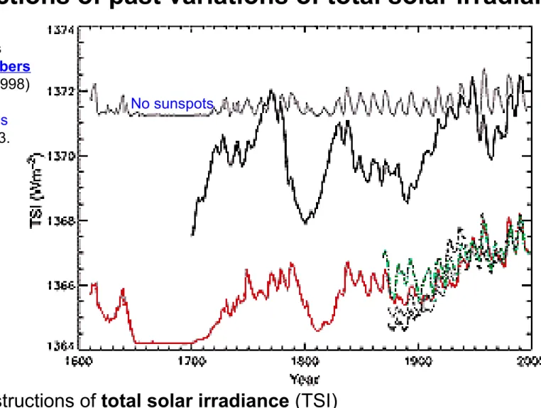
Reconstructions of past variations of total solar irradiance

Fig. 6.5: Reconstructions of total solar irradiance (TSI)

by Lean et al. (1995, solid red curve),

Hoyt and Schatten (1993, data updated by the authors to 1999, solid black curve), Solanki and Fligge (1998, dotted blue curves),

and Lockwood and Stamper (1999, heavy dash-dot green curve);

The grey curve shows group sunspot numbers (Hoyt and Schatten, 1998) scaled to

Nimbus-7 observations for 1979 to 1993.

No sunspots

(20)

Die Sonnenleuchtkraft in der Erdgeschichte

Im Laufe der Erdgeschichte hat sich die Leuchtkraft der Sonne um knapp

+10 % pro Ga

erhöht. [Ga= Giga Jahr] . Diese Entwicklung wird sich in den nächsten fünf Milliarden Jahren fortsetzen.

Dieser Anstieg resultiert aus der wachsenden Wasserstoff-Verbrennungsrate während der Hauptreihen-Entwicklungsphase der Sonne. Ein Stern

befindet sich in dieser Phase, wenn er sich im hydrostatischen Gleichgewicht befindet und in seinem Innern eine stabile Kernfusion läuft.

Wie sich die Leuchtkraft eines Sterns in Abhängigkeit von seiner Masse entwickelt, lässt sich mit heutigen Sternentwicklungsmodellen berechnen (+1_Folie). Die Ergebnisse für die Leuchtkraft als Funktion der effektiven Strahlungstemperaturen werden in einem Hertzsprung-Russell-Diagramm dargestellt (siehe "Das Hertzsprung-Russell- Diagramm", +2_Folie)

und gehen in die Berechnung des Klimamodells ein.

Bounama,C. e.a.: „Auf der Suche nach einer zweiten Erde“; PhiuZ 33 (2002),p.122 -128; p.123

(21)

Hertzsprung-Russell-Diagramm

für Sterne mit 0,8 bis 2,5 M

_S

(M

_S

= Sonnenmasse) [2].

Es wird nur die Entwicklung auf der Hauptreihe dargestellt.

Die aufeinander folgenden Punkte der massenspezifischen Kurven stellen Zeitschritte von 1 [Ga] dar.

Der heutige Entwicklungsstand

unserer Sonne ist durch einen roten Punkt hervorgehoben.

Unsere Sonne: 1,0 M

_S

Leuchtkraft =

absolute Helligkeit

Die Leuchtkraft der Sonne im Laufe von GigaJahren

Die frühe Sonne strahlte 30% weniger Energie

Bounama,C. e.a.: „Auf der Suche nach einer zweiten Erde“; PhiuZ 33 (2002),p.122 -128; Abb.2; p.124

(22)

In einem Hertzsprung-Russell-Dia gramm sind die Ster- ne entsprechend ihrer Spektralklasse und ihrer Leucht- kraft eingetragen.

Der Leuchtkraft entspricht eine absolute Helligkeit,

der Spektralklasse eine effektive Strahlungstemperatur.

Es handelt sich damit um ein Zustandsdiagramm.

Diese Darstellungsform wurde 1913 von dem amerikanischen Astronomen Henry Norris Russell gewählt, nachdem sein dä- nischer Kollege Einar Hertzsprung 1905 entdeckt hatte, dass es unter Sternen gleicher Temperatur Riesen und Zwergsterne gibt.

Das Hertzsprung-Russel'-Diagramm ist nicht gleich- mäßig besetzt. Vielmehr ordnen sich die Sterne in bestimmten Gebieten oder »Ästen" an.

Die Mehrzahl der Sterne liegt auf einem relativ scharf begrenzten Ast. den man als Hauptreihe bezeichnet.

Auch unsre Sonne ist ein Hauptreihenstern.

Sterne entwickeln sich mit der Zeit und damit ändern sich hre Werte für Leuchtkraft und effektive Strah-

lungstemperatur. Daher wandert der Bildpunkt im Hertzsprung-Russell- Diagramm im Laufe der Zeit:

Er legt einenn „Entwicklungsweg" zurück..

Das Hertzsprung-Russell Diagramm

Schematische Darstellung eines

Hertzsprung-Russel'- Diagramms.

( Strahlungstemperatur)

Bounama,C. e.a.: „Auf der Suche nach einer zweiten Erde“; PhiuZ 33 (2002),p.122 -128; p.127 Infokasten

(23)

_1 Der Sonnenvektor oder „wo steht die Sonne“

_11 Zeitgleichung,

_12 Azimut und Sonnenhöhe

_13 Direkte Solare Inzidenz auf geneigte Fläche

_2 Streuung und Absorption der Solarstrahlung

_1 Angström‘s turbidity _2 Linke‘s Trübungsfaktor _3 Parametrisierung [Kasten 95]

_3 Diffuse und direkte Solarstrahlung

_20 Strahlungsgrößen

_21 Anteil der diffusen Strahlung an der Globalstrahlung /Reindl e.a.1990/

_22 Perez-Modell: die anisotrope Himmelsstrahlung /Perez e.a. 1990/

3.22 Solare Einstrahlung

(24)

Wo steht die Sonne

_1 Der Sonnenvektor

_

11 Zeitgleichung,

_

12 Azimut und Sonnenhöhe

_

13 Direkte solare Inzidenz auf geneigte Fläche

3.221

(25)

The earth‘s orbit

(shown with an exaggerated eccentricity )

the mean orbital distance is a = 149,7 [Gm] = 149,7 Mio km and the eccentricity is  = 0.0167

also ca. :: r = a +- 1,7%

cos  = -1  =0 ; cos  =+ 1

r

_a

= r

_Aphelion

=a (1+  ) r

_p

= r

_Perihelion

=a (1-  )

Wdh aus 3.21

Zur Erinnerung: Elliptische Erdbahn. also:

Winkelgeschindigkeit nicht genau gleichförmig

3.2211 Zeitgleichung

(26)

BQuelle: Strahler: „Physical Geography“,2002, Wiley-Verlag, ISBN=0-471-23800-7, Bild3.2,p.37; (ein Buch mit wunderschönen Bildern) IG4e_01_02

The direction of the Earth’s rotation is

counterclockwise or West to East

The direction of the Earth’s rotation is counterclockwise when viewed from above the north pole

or west to east

when viewed with the north pole up.

(27)

viewed from a point over the Earth’s north pole:

Earth and Moon both rotate and revolve in a counterclockwise direction

Alles läuft und dreht sich im mathematisch positivem Sinne

BQuelle: Strahler: „Physical Geography“,2002, Wiley-Verlag, ISBN=0-471-23800-7, Bild3.14,p.54;

(28)

1. Sterntag: die Erde dreht sich einmal um ihre Rotationsache (in einem im Fixsternensystem verankerten Bezugssystem.

Drehrichtung: rechte Handregel

2. Wenn sich die Erde nicht um ihre Achse drehen würde, so gäbe es dennoch einen „Umlauftag“ wegen des Umlaufes um die Sonne und dieser würde genau ein Sonnenjahr dauern.

Diese Rotation durch Umlauf um die Sonne wirkt jedoch gegenläufig zur Eigenrotation . 3. Sonnentag: Die Erde dreht sich einmal um sich selbst (Sterntag) + zusätzlich noch ein

bißchen weiter um den gegenläufigen Dreheffekt des Umlaufes um die Sonne wieder auszugleichen .

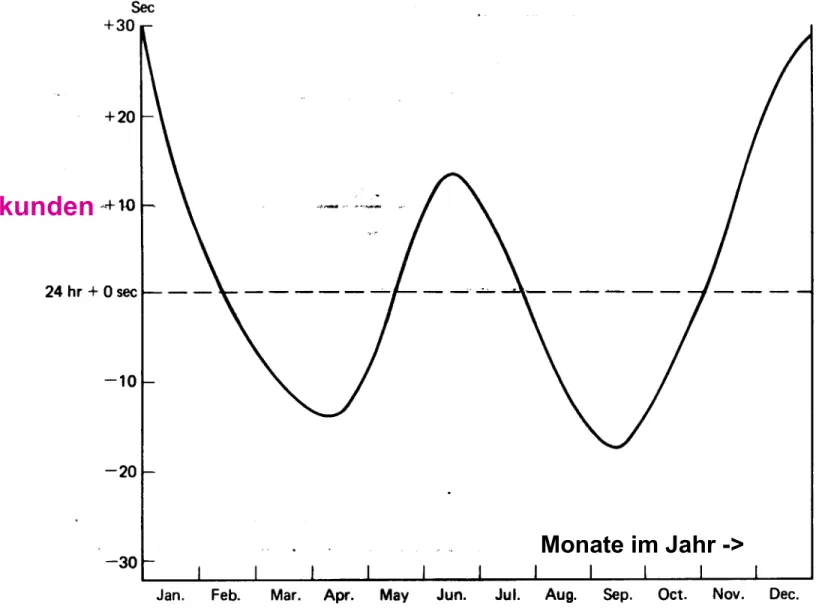
4. Der Umlaufwinkel während eines Sterntages ist allerdings auf der elliptischen Erdumlaufbahn etwas ortsabhängig. Daher ist die Zeitdauer des Sonnentages veränderlich und zwar in einem Bereich von +30sec bis -20 sec um den mittleren Sonnentag.

5. Zeitgleichung = die kumulierten Abweichungen vom mittleren Sonnentag.

Zum Verständnis der Zeitgleichung

(29)

2. Eine Vierteldrehung der Richtung zur Sonne durch Eigenrotation der Erde in 6 h

Sonne

1. Eine Vierteldrehung der Richtung zur Sonne durch ¼ Jahr auf der Umlaufbahn:

Sonne

12 Uhr Position (Start)

6 Uhr Position des roten Pfeiles

12 Uhr (Start)

18 Uhr (6h später)

Veranschaulichung:

DrehRichtung zur Sonne bei Jahresumlauf und bei Eigenrotation der Erde

G.Luther, Uni Saarbrücken

¼ Jahr später

(30)

FIGURE 2.3 The seasonal deviation of the app arent solar day about the mean solar day

Die wahre Tageslänge:

Differenz zur mittleren Tageslänge

^{(=24 h)}

Quelle: Sol Wieder:“An Introduction to Solar Energy for Scientists and Engineers“,Wiley, NewYork 1982, ISBN=0-471-06048-8, Figure 2.3, p.24

Monate im Jahr ->

Sekunden

(31)

Minuten

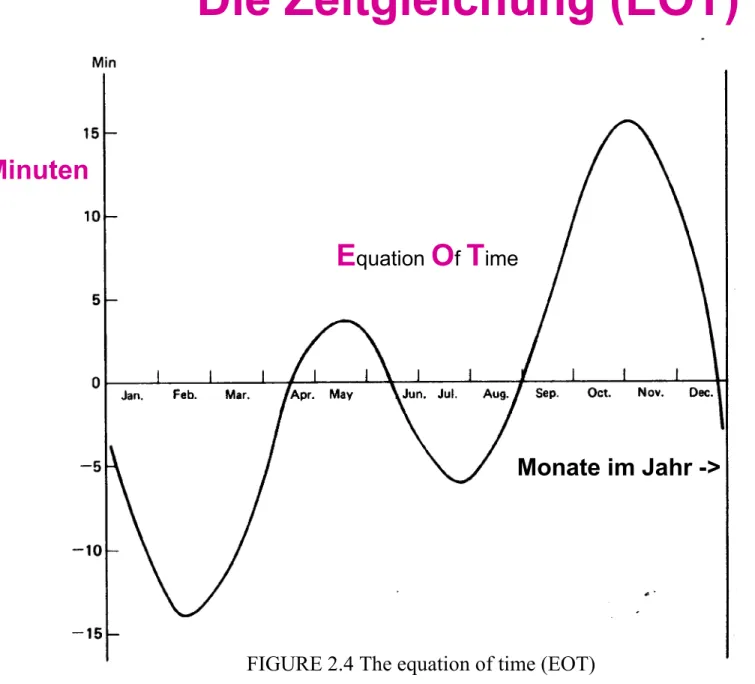
Quelle: Sol Wieder:“An Introduction to Solar Energy for Scientists and Engineers“,Wiley, NewYork 1982, ISBN=0-471-06048-8, Figure 2.4, p.25

FIGURE 2.4 The equation of time (EOT)

Die Zeitgleichung (EOT)

E

^quation

O

^f

T

^ime

Monate im Jahr ->

(32)

Quelle: Sol Wieder:“An Introduction to Solar Energy for Scientists and Engineers“,Wiley, NewYork 1982, ISBN=0-471-06048-8, Table2.1, p.26

Die Zeitgleichung (EOT)

DIN Algorithmus (DIN 5034):

(zitiert nach Quaschning: „Regenerative Energiesysteme“, 2.Auflage, Gl. 2.15, p..53)

Sei

J‘ = 360° * [Tag des Jahres / Zahl der Tage im Jahr] „Tageswinkel imJahr“

EOT in [min] = 0,0066 + 7,3525 *cos( J‘ +85,9°) + 9,9359 * cos ( 2*J‘ + 108,9°) + 0,3387* cos( 3*J‘ + 105,2°)

(33)

Quelle:Quaschning: „ Regenerative Energiesysteme“, 2.Auflage, p..53)

Höhe

und

Azimut

der Sonne

DIN 5034 Algorithmus:

Azimut nach DIN:

0° = Norden (ungewöhnlich)

90° = Osten (Uhrzeigersinn)

3.2212 Azimut und Sonnenhöhe

(34)

Veranschaulichung der scheinbaren Sonnenbewegung - am Nordpol

- am Äquator

- in mittleren Breiten

(35)

Am Nordpol

BQuelle: Strahler: „Physical Geography“,2002, Wiley-Verlag, ISBN=0-471-23800-7, Bild4.9,p.80; (bzw. [IG4e_02_09]

(36)

Am Äquator

the sun’s path across the sky varies in position and height above the horizon seasonally (equator)

BQuelle: Strahler: „Physical Geography“,2002, Wiley-Verlag, ISBN=0-471-23800-7, Bild4.7c,p.79; (bzw. [Fig.2.7c, p.58] )

(37)

Equinoxes - at noon the Sun is 50 degrees above horizon Solstices -

June solstice has a higher angle than the December

solstice

In mittleren Breiten (40 °N)

BQuelle: Strahler: „Physical Geography“,2002, Wiley-Verlag, ISBN=0-471-23800-7, Bild4.7b,p.79; (bzw. [Fig.2.7b, p.58] )

(38)

Urquelle: e.g. Bourges: Climatic Data Handbook for Europe 1992, p.8; Quelle: SolareEinstrahlung.doc

3.2213 Solare Inzidenz auf geneigte Fläche

Sonnenstand und Orientierung des Kollektors

N W



S

Zenith



Normal to Collector plane

Collector azimuth Solar height 

Solar azimuth

Sun

S_vekt

n_vekt

(39)

UrQuelle: z.B. V. Quaschning 2003: Regenerative Energiesysteme (3.A.), p.54, - man beachte jedoch obige Bem. 2.

Sonnenstand und Orientierung des Kollektors

N W



S

Zenith

 Normal to

Collector plane

Collector azimuth Solar height  Solar azimuth

Sun S_vekt n_vekt

s_vekt = Einheitsvektor in Richtung Sonne n_vekt = FlächenNormale (Einheitsvektor) des Kollektors

Sei



= Winkel(s_vekt,n_vekt )

Betrachte Skalarprodukt : s_vekt*n_vekt

 = arccos(s

_vekt

* n

_vekt

)

Darstellung der Vektoren in Cartesichen Koordinaten

und Ausrechnung des Skalarproduktes ergibt:

 = arccos { + cos 

_s

* sin 

_K

* cos( 

_s

- 

_K

) + sin 

_s

* cos 

_K

}

Index: s=Sonne, K=Kollektor



Bem.: 1. Da die Differenz der Azimutwinkel von Kollektor und Sonne gebildet werden ist der Nullpunkt (Süd oder Nord) unerheblich 2. Man achte jedoch auf die Definition des Kollektorazimuts, der hier der Azimut der FlächenNormale ist

3. Wird der Azimutwinkel des Kollektorschenkels, _K‘ = _K +



, genommen, muss der 1.Term

„

-

cos 

_{s ….}

“

heißen.

(40)

Streuung und Absorption der Solarstrahlung

- Optische Dicke



_R

(m) d

er reinen und trockenen Atmosphare ( nur Rayleigh Streuung)

- Linke‘s Trübungsfaktor T_L

- Parametrisierung von T_L(m) [Kasten 95]

3.222

(41)

Einfallende Solarstrahlung und Transmission durch Atmosphäre

Quelle:V. Quaschning 2003: Regenerative Energiesysteme(3.A.), Hanser Verlag München, ISBN=3-446-24983-8, Bild 2.3,p45

Solarkonstante:

I

₀

= 1367 [W/m

²

]

(42)

Extinktionsvorgänge

(Absorption und Streuung)

in der Erdatmosphäre

(schematisch)

1 -> 1‘ : Absorption durch Ozon

1‘ -> 2 : Streuung an Molekülen der Luft (Rayleigh Streuung)

2 -> 3 : Streuung und Absorption an Aerosolpartikeln (Mie-Str.)

3 -> 4 : Absorption durch Wasserdampf

UrQuelle: Fritz Kasten: „Beiträge zum Strahlungsklima –insbesondere SW-Deutschlands“,Manuskript zu Vortrag am 2.6.1987 in Saarbrücken; Fig.1 (red. bearbeitet)

unter wolkenlosem Himmel

(43)

Optische Dicke der Atmosphäre: Linke‘s Trübungsfaktor T

_L

UrQuelle: Fritz Kasten: „Beiträge zum Strahlungsklima –insbesondere SW-Deutschlands“,Manuskript zum Vortrag am 2.6.1987 in Saarbrücken; p.2+3)

1.

Wegen der starken Wellenlängenabhängigkeit von Streuung und Absorption der Solarstrahlung ist die optische Dicke der Atmosphäre eine spektrale Größe:

(



)

.

Bei nicht zu hohen Genauigkeitsansprüchen kann man jedoch mit einer spektral gemittelten optischen Dicke

 rechnen

^.

Bei Vernachlässigung der Mehrfachstreuung lässt sich dann

die Extinktion der direkten Sonnenstrahlung

I

in der Atmosphäre beschreiben durch:

I = I

₀

* exp{-  * m) (1)

(Gesetz von Bouquer-Lambert)

mit der „airmass“ m = relative Länge der durchstrahlten Luftmasse

im Vergleich zum senkrechten (m=1) Einfall.

2.

Aus praktischen Gründen normiert man



auf eine Bezugsgröße



_R, nämlich auf die optische Dicke einer reinen und trockenen Atmosphäre,

in der nur Rayleigh- Streuung an den Molekülen der Luft stattfindet.

Diese „integrale Rayleigh optische Dicke“



_R kann man unter Standardbedingungen berechnen, wobei noch eine Abhängigkeit von der Luftmasse m übrig bleibt:



_R

(m)

3. Die Trübung der Atmosphäre lässt sich dann beschreiben durch den „Linke‘ schen Trübungsfaktor T

_L

mit:  = T

_L

* 

_R

(2)

Aus (1) und (2) folgt dann:

I = I

₀

* exp{- T

_L

* 

_R

* m) (3)

(44)

UrQuelle: Fritz Kasten: „Beiträge zum Strahlungsklima –insbesondere SW-Deutschlands“,Manuskript zum Vortrag am 2.6.1987 in Saarbrücken;Abb. 31)

Trier 1979-1986 :

Der Linke‘sche Trübungsfaktor mit Schwankungsbreite

Die Bestimmung der Trübung erfolgt nur aus Messungen in wolkenlosen Stunden : G (0) und D (0)

Es gilt :

G(0) - D(0) = B(0) = I(0)*sin  mit  = Sonnenhöhe zur Stundenmitte

Bestimmung durch Vergleich mit Gl.(3):

^{I(0) = I}

₀

^{* exp{- T}

_L

**^{* }**

_R

* m) (3)

Die große Schwankungsbreite

rührt von den Luftmassenwechsel her.

(45)

Woher bekommt man die Werte für Rayleigh optische Dicke 

_R

her?

Parametrisierung der Rayleigh optischen Dicke 

_R

Fritz Kasten: „The LinkeTurbidity Factor based on Improved Values of the integral Rayleigh Optical Thickness“; SolarEnergy 56 (1996); p. 239.pdf



_R

(m)

theoretisch berechnet

und

parametriesiert

(equ. 10 ist ok)

(46)

…? Antwort: aus der Parametrisierungsformel (10) von Kasten (1996) :

Fritz Kasten: „The LinkeTurbidity Factor based on Improved Values of the integral Rayleigh Optical Thickness“; SolarEnergy 56 (1996); p. 239.pdf

Neue theoretische Berechnung mit spektraler Integration

(47)

Diffuse und direkte Solarstrahlung

3.223

(48)

Recommendations for units and symbols in Solar Energy

Urquelle: International Journal of Solar Energy , 1984, V 01. 2, pp. 249- 255.

Quelle: e.g. / Palz-Greif 96: European Solar Radiation Atlas , Table A.1.2, p.41+42 /

Empfohlene Symbole:

Unterteilung der Solarstrahlung : G = Global irradiation S = Sunshine duration I = Direct irradiation (direct beam)

D = Diffuse irradiation

subscripts for indicating the time period over which the irradiation is incident : h = hourly; d= daily,

m = monthly mean daily z.B. G_time

further subscripts: 0 = extraterrestríal or astronomical

c = clear sky ; b = bedeckt, overcast ; g = ground In der Meteorologie bezeichnet man als:

Solar radiation = spectral range between 0.29 µm and 4 µm . Umfasst 99% der auf die Erdoberfläche auftreffenden Strahlung )

Terrestrial Radiation = spectral range above 4 µm

Bezeichnung: Irradiance = < power per unit area > = [ W /m² ] = Bestrahlungsstärke Irradiation = < energy per unit area > = [ Wh /m² ] = Einstrahlung

Angaben beziehen sich in der Regel auf die Flächeneinheit

3.2230 Strahlungsgrößen

(49)

Solare Bestrahlungsstärke und Einstrahlung

e.g. / Palz-Greif 96: European Solar Radiation Atlas , Table A.1.2, p.44 /

Direct beam I (irradiance)

Term Symbol Definition Unit

---

direct irradiance

I

direct solar irradiance normal to beam W /m²

I(ß, )

direct irradiance on plane of slope ß and azimuth 

...

Extraterrestrial

I

_{o j} Extraterrestrial solar irradiance normal to beam irradiance on day j

Solar constant

I

_o Annual mean value of the

extraterrestrial normal irradiance Value used 1370 W /m^{2 .} (1367 W/m²)

...

Hourly

I

_h Hourly integral of direct irradiance normal to beam W h /m² direct irradiation

Daily

I

_d Daily integral of direct irradiance normal to beam direct irradiation

Monthly mean

I

_m Monthly mean of daily direct irradiation normal to beam direct irradiation

(50)

Solare Bestrahlungsstärke und Einstrahlung

Diffuse radiation D ( diffuse )

---

Diffuse irradiance

D

Irradiance from the sky W /m²

D(ß, )

Irradiance from the sky and from the ground (for tilted planes)

...

Clear sky

D

_c Irradiance from clear sky diffuse irradiance

Overcast sky

D

_b Irradiance from overcast sky

diffuse irradiance (bewölkt)

...

Hourly

D

_h Hourly integral of irradiance from the sky W h /m²

diffuse irradiation

Daily

D

_d Daily integral of irradiance from the sky diffuse irradiation

Monthly mean

D

_m Monthly mean of daily irradiation from the sky diffuse irradiation

(51)

e.g. / Palz-Greif 96: European Solar Radiation Atlas , Table A.1.2, p.44+45 /

Global radiation G ( global )

---

Global irradiance

G

Global irradiance: Sum of diffuse and direct irradiance W /m² on any receiving plane.

G(ß, )

Global irradiation on plane of slope ß and azimuth  (sum of irradiance from the sun, the sky and the ground)

...

Clear sky

G

_c Global irradiance under clear sky global irradiance

Overcast sky

G

_b Global irradiance under overcast sky ,

G

_b

= D

_b

global irradiance (bedeckt)

...

Hourly

G

_h Hourly integral of global irradiation W h /m²

global irradiation

Daily

G

_d Daily integral of global irradiation global irradiation

Monthly mean

G

_m Monthly mean of daily global irradiation global irradiation

...

Monthly mean

G

_0m Monthly mean of daily extraterrestrial global irradiation extraterrestrial

global irradiation

Solare Bestrahlungsstärke und Einstrahlung

(52)

Irradiance

W/ m²

On

inclined

plane:

W/ m²

 = slope

 = azimuth

hourly Integral Wh/ m²

irradiation

daily Integral Wh/ m²

irradiation

monthly Integral

Wh/ m²

irradiation

Direct beam

direct: I

normal to beam

I( ,  ) Ih Id Im

Diffuse radiation

diffuse: D D( ,  ) D_h D_d D_m Global radiation

global: G G( ,  ) G_h G_d G_m

e.g. / Palz-Greif 96: European Solar Radiation Atlas , Table A.1.2, p.44 / Solare Bestrahlungsstärke und Einstrahlung: Übersicht

(53)

Sehr häufig findet man jedoch eine weniger systematische Bezeichnung zur Unterteilung der Solarstrahlung, z.B. :

G = Global irradianc [W/m^2]

statt I : G

_b

= Direct irradiance (direct beam )

statt D: G

_d

= Diffuse irradiance

(54)

Angles of the location



Latitude, North positive.



Longitude, East of Greenwich positive Angles of collector plane



Azimuth angle of a plane, i.e. the angle between

the projection of the normal on the horizontal plane and true south in northem hemisphere,

(or true north in southem hemisphere).





Inclination angle of a plane with respect to the horizontal plane.

Time and date (Solar hour angle and declination)



Solar hour angle, measured from solar noon: p.m. is positive.



Solar decIination, i.e. the angle between the sun's rays and the equatorial plane.

Angles of the sun



_s Solar elevation, i.e. altitude angle above horizon.



Solar azimuth, measured from true south in northem hemisphere:

west of south positive, east of south negative.



Solar zenith angle, i.e. angle between the centre of the sun's disc and the vertical.



=

 /

2

- 

;



(



,



) Angle of incidence between the sun's rays and an inclined plane.

Geometrie von Sonne und Kollektorebene

(55)

Der mittlere Anteil der diffusen Strahlung an der Globalstrahlung, D_Faktor, kann über statistische Erfahrungswerte geschätzt werden.

Hierbei werden als Parameter benutzt:

kt

_h

= Stundenwert des Klarheitsindexes ,

und

Sin(

_s

) = Sinus der Sonnenhöhe 

_s

(genommen in der StundenMitte)

( wobei kt_h = G_h(0) / I_0h(0) =die horizontale auf die extraterrestrische Strahlung I₀(0) = I₀ *Sin(



_s) normierte Stundensumme der Globalstrahlung ist )

Korrelation nach /Reindl-Duffie- Beckman 1989/:

If kt_h <= 0.3 Then

D_Faktor = 1.02 - 0.254 * kt_h + 0.0123 * Sin(

_s

)

ElseIf kt_h < 0.78 Then

D_Faktor = 1.4 - 1.749 * kt_h + 0.177 * Sin(

_s

)

Else

D_Faktor = 0.486 * kt_h - 0.182 * Sin(

_s

)

End IF

Die geschätzte Diffus-Strahlung beträt dann:

D

_h

(0) = D_Faktor * G

_h

(0)

Bestimmung der diffusen Komponente aus der Globalstrahlung

BQuelle: z.B. V. Quaschning 2003: Regenerative Energiesysteme (3.A.), p.50,

3.2231

(56)

Diffuser Strahlungsanteil (D_Faktor) ,

nach /Reindl-Duffie-Beckman90/

Quelle: V. Quaschning 2003: Regenerative Energiesysteme (3.A.), Bild 3.8, p.51

(57)

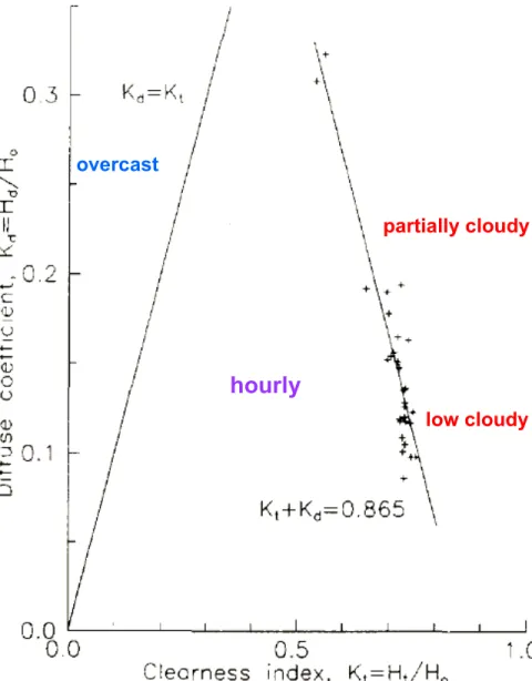
Kd(kt) Darstellung , Perez et.al. 1991

4 Zonen:

- Kd=kt - Übergang - Kd +Kt =C - K

(58)

Vasquez-Ruiz-Perez (1991): „The Roles_of Scattering, Absorption and Air Mass on the Diffuse-to-Global Correlations“; SolarEnergy 47, p181

(59)

Fig. 6. Plot of hourly Kd vs. Kt for the 11 a.m. to 1 p.m. period of all the days of September 1980 for Madrid.

Also plotted is eqn (3)

^K

_t

^{+ K}

_d

= C (3)

fitted for the data.

hourly

Common Shape of Kd-Kt -Curves

overcast

partially cloudy

low cloudy

(60)

Effect of the bimodal

(=clear-cloudy)

behaviour on the Kd vs. Kt relationship

Vasquez-Ruiz-Perez (1991): „The Roles_of Scattering, Absorption and Air Mass on the Diffuse-to-Global Correlations“; SolarEnergy 47, p.181; Fig. 11

K

_d

K

_t

2 3 1 4

Zone 4: periods of unshaded suns in partly cloudy skies.

(seen only in short time measurements)

Zone 2: Overcast sky: K_d = K_t

Zone 1: periods of unshaded suns in low cloudy skies.

50% of light stopped by cloud should be scattered downwards K_t + K_d =C

Zone 3: Übergang

short time m.

(61)

Das Perez Modell

der anisotropen diffusen Himmelsstrahlung

3.2232

(62)

Source:

eine preisgekrönte zusammenfassende Darstellung

Quelle: Perez e.a. / PISMS90/ :“Modeling…Components from Direct and Global Irradiance“.SolarEnergy 44,p271,(1990)

(63)

Quelle: Perez, Richard e.a. / PISMS90/ :“Modeling…Components from Direct and Global Irradiance“.SolarEnergy 44,p271,(1990)

(64)

Wir betrachten zuerst das ursprüngliche „physikalische“ Perez- Modell der Himmels –Halbkugel.

Aus rechnerischen Gründen wurde dieses Modell dann vereinfacht und „abstrakter“.

Quelle: Perez,R. e.a. /PSASS86/:“ Anisotropic hourly-diffuse Radiation Model for SlopingSurfaces“ SolarEnergy 36, p481, (1986).pdf

(65)

Quelle: Perez,R. e.a. /PSASS86/:“ Anisotropic hourly-diffuse Radiation Model for SlopingSurfaces“ SolarEnergy 36, p481, (1986). p.481

The model is composed of three distinct elements:

(

^§

1) Geometrical representation of the sky dome,

(

§

2) Parametric representation of the insolation conditions,

and

(

^§

3) Statistical component linking (1) and (2) .

Der dreifache Pfad des Perez Modells

(66)

Quelle: Perez,R. e.a. /PSASS86/:“ Anisotropic hourly-diffuse Radiation Model for SlopingSurfaces“ SolarEnergy 36, p481, (1986), Fig.1, p.482

(

^§

1) Model geometrical representation of the sky hemisphere.

3 Himmels - Bereiche:

1. Circumsolar Brightening

2. Horizon Brightening

3. main portion (Hintergrund)

1 

^=15°



=6.5°

2 2 2 2

2 2 2

2

Model accounts for the two main zones of anisotropy:

1. Circumsolar Brightening , due to forward scattering by aerosols. Factor

F1

for additional brightening.

2. Horizon Brightening , due primarily to multiple Rayleigh scatterimg

and retroscattering in clear atmospheres. Faktor

F2

for additional brightening.

(67)

L = Radiances originating from the main portion of the dome, **F1 * L = ~ ~ from the circumsolar zone,**

F2 * L = ~ ~ from the horizon zone

 = the half angle of the circular region centered on the sun's position = set at 15 ° for the model studied here.

 = is the horizon band angular thickness, = set at 6.5 ° for the presented model.



= solar incidence angle on the considered plane

(= Winkel zwischen Flächenvektor und Sonnenstrahl) Not indicated in the picture:

angle z' = the solar zenith angle, z, if the circular region is totally visible,

= its average incidence angle, if the circular region is only partially visible.

s = „slope“ angle , the plane‘s tilt angle

Nomenclature:

(68)

Diffuse irradiance from the sky dome

a . Diffuse irradiance Dh on the horizontal plane

**isotropic contribution from the whole semi-sphere = L * { 2 }**

**additional contribution from circumsolar brightening = L(F1 -1) { 2 * c( , z) }** additional contribution from horizon brightening = L(F2 -1) { 2 * d(  ) } thus:

Dh = 2 L * [ 1 + c(, z)* (F1 -1) + d()* (F2 -1) ]

,whereby

c( , z) and d(  )

are the solid angles occupied by the two anisotropic regions,

weighted by the average incidence on the horzontal plane.

(69)

b) Diffuse irradiance Dc on the plane of slope s

**isotropic contribution from the „seen“ sphere = L * { 2 * 0.5*(1+cos(s) )}**

**additional contribution from circumsolar brightening = L(F1 -1) { 2 * a( ,  ) }** additional contribution from horizon brightening = L(F2 -1) { 2 * b( ,s ) } thus:

Dc = 2 L * [ 0.5*(1+cos(s) ) + a(,  **)*(F1 -1) +** b( ,s) * (F2 -1) ]

,whereby

a( , z ) and b(  )

are the solid angles occupied by the two anisotropic regions,

weighted by the average incidence on the slope s.

(70)

Bemerkung:

Was (= welchen Raumwinkel) sieht eine geneigte Fläche bei isotroper Einstrahlung?

s

Vollständiger Halbraum: 2*



Halbseitiger Halbraum (Viertelraum):



Die geneigte Fläche

sieht die (rechte) sonnenseitige Häfte des Halbraumes vollständig und die „schattige“ Hälfte des Halbraumes zum Bruchteil cos(s).

also sieht sie den Raumwinkel: (1 + cos(s)) *



(Vor. Isotrope Einstrahlung, „Lambertstrahler“)

Einschub

s

(71)

Ratio of the diffuse irradiances

a) Diffuse irradiance Dh on the horizontal plane

Dh = 2 L * [ 1 + c(, z)* (F1 -1) + d()* (F2 -1) ] b) Diffuse irradiance Dc on the plane of slope s

Dc = 2 L * [0.5*(1+cos(s) ) + a(,  )*(F1 -1) + b( ) *(F2 -1) ]

c) thus: Dc = Dh * [ 0.5(1+cos(s) ) + a(,  )(F1 -1) + b(,s ) (F2 -1) ] [ 1 + c(, z) (F1 -1) + d()* (F2 -1) ]

From the solar geometry and the slope of the plane the solid angle a, b, c and d can be calculated.

F1

and

F2

must be empirically evaluated from the statistics of measurements of Dc and Dh from different sites and at well defined „Sky conditions“.

The classification of comparable „sky conditions “ is given in the next paragraph (§2).

equ.(4)

(72)

Quelle: Perez,R. e.a. /PSASS86/:“ Anisotropic hourly-diffuse Radiation Model for SlopingSurfaces“ SolarEnergy 36, p481, (1986), p.482

Appendix : Citation of the geometrical parameters:

Equation (6)

The parameter Xh is the fraction of this circular region

which is seen by the horizontal,

and the parameter Xc is the equivalent of Xh for the tilted plane

(73)

(§2) Parametric representation of the insolation conditions

The sky condition parameterization (vorläufig!!):

Considering that the calculation of irradiance on a slope at a given instant requires the knowledge of:

• the normal incidence direct irradiance,

• the horizontal diffuse irradiance, and

• the solar position,

the three following variables are used to describe the actual type of sky condition:

•  = (Dh + l )/Dh, where I is the normal (!) incidence direct radiation

• Dh, horizontal diffuse radiation

• z, solar zenith angle

It is assumed, at this stage of model development, that z, Dh and  are independent quantities defining a 3-dimensional space.

This space is divided into over 200 "sky condition categories," by defining intervals for each of the variables. These are presented in Table I.

(74)

Description of the intervals depicting the sky conditions

Quelle: Perez,R. e.a. /PSASS86/:“ Anisotropic hourly-diffuse Radiation Model for SlopingSurfaces“ SolarEnergy 36, p481, (1986),Table 1,p.483

Vorläufig, nur zum Verständnis, gerechnet wird heute mit einem modifizierten und vereinfachten Modell

Dh  z

(75)

The sky condition~model configuration relationship.

The only undefined terms in equ.(4) are the coefficients F1 and F2.

Zur Erinnerung: Equ.(4)

Dc = Dh * [ 0.5(1+cos(s) ) + a(,  )(F1 -1) + b(,s ) (F2 -1) ] [ 1 + c(, z) (F1 -1) + d()* (F2 -1) ]

These non-dimensional multiplicative factors ,

F1 and F2 ,

set the radiance magnitude in the two anisotropic regions relatively to that in the main portion of the dome.

The degree of anisotropy of the model is a function of these two terms only.

The model can go from an isotropic configuration (F1, F2 = 1)

to a configuration incorporating circumsolar and/or horizon brightening.

(76)

The sky condition~model configuration relationship (Forts).

The magnitude of these coefficients, F1 and F2 , is treated as a function of the three variables describing the sky conditions:

 = (Dh + l )/Dh,

Dh

z = solar zenith angle

At this stage of model development, these are not continuous functions, but matrices corresponding to the

discrete partition of the sky condition space

presented above,

i.e. the

[z, , Dh] intervals

.

(77)

(§3) Statistical component linking (§1) and (&2)

These coefficients , F1 and F2, constitute the statistical/experimental part of the model.

Measurements:

They are obtained through the analysis of hourly--or higher frequency--

data recorded

^with

ground-shielded pyranometers of

different slopes and orientations

.

In order not to bias the model in favor of a specific orientation, measurements are needed

in the four cardinal directions

.

Also one or more sloping, south-facing or sun-tracking measurements are needed.

The analysis consists of

optimizing F1 and F2 for each [z, , Dh] interval

by least square fitting of measured data.

(78)

Die endgültige, vereinfachte und abstraktere Fassung des Perez Modells

(79)

(80)

Tracking PV - modules

Was bringt es , wenn der PV-Modul der Sonne nachgeführt wird.

Vollständige Nachführung muss 2-achsig sein.

Aber bereits eine 1-achsige Nachführung bringt fast den ganzen Vorteil.

3.2233

(81)

Source:

Quelle:Nann,S.: „Potentials for Tracking PV Systems and V-Troughs in Moderate Climates“, SolarEnergy 45, p.385, (1990)

Calculations are based on the Perez model !

(82)

Betrachte: One-axis Tracker

Azimuth tracker with a vertical axis

and fixed inclination  of the module

 S

 N

Azimuth tracker with a North-South axis

and fixed inclination  of the module

Sun

(83)

Yearly Irradiance received for different Trackers

Irradiance during one year relative to the

40° optimum tilted fixed array

(i) for a fixed array with varying inclination,

(ii) an azimuth tracker with a vertical axis and varying inclination of the modules,and

(iii) an azimuth tracker with N-S axis and different angles of inclination of the entire axis.

Based on measurements in

Weihenstephan, Germany

Latitude: 48°N

Inclined axis tracker

Fixed array

Calculated

with the Perez-model

Quelle:Nann,S.: „Potentials for Tracking PV Systems and V-Troughs in Moderate Climates“, SolarEnergy 45, p.385, (1990), Fig1, (redaktionell bearbeitet)

flat vertical



(84)

•Based on hourly monthly means of global and diffuse radiation [15], Fig. 1 shows

the irradiation received by differently oriented surfaces.

In Fig. 1

the irradiance received during one year from the 40” tilted fixed array is compared with:

(i) the amount received, when the tilt angle of the

fixed array

differs from this optimum value.

In the same way the graph shows two

one-axis systems

^with:

(ii) the vertical-axis tracking system with inclination



of the modules varying from 0° to 90°, and

(iii) its tilted tracking axis with tilt angle



varying from 0° to 90°

• From Fig. 1 one can conclude the

optimum angle of inclination 

for modules and axes to receive the highest amount of radiation at Weihenstephan (F.R.G.).

• Applying the Perez model, the surplus of energy due to tracking stems to about

one third from the circumsolar radiation

^.

Original (nearly) description of Fig.1

Quelle:Nann,S.: „Potentials for Tracking PV Systems and V-Troughs in Moderate Climates“, SolarEnergy 45, p.385, (1990),p.386 (redaktionell bearbeitet)

(85)

Mean annual irradiance received by different tracking arrays

Quelle:Nann,S.: „Potentials for Tracking PV Systems and V-Troughs in Moderate Climates“, SolarEnergy 45, p.385, (1990),Table 1,p.387 (redaktionell b.)

Cell

: Irradiance is reduced by transmission-losses, because of reflection losses and absorption losses through the module cover for both diffuse and direct irradiance .

Calculation: with a completed version of the Perez model

and hourly monthly radiation data on a horizontal surface for the years 1979-1986.

The values are relative to the irradiance upon a fixed 40° array

cell

(only solar height angle is tracked) (azimuth tracker)

(azimuth and solar height are tracked) Based on measurements in

Weihenstephan, Germany Latitude: 48°N

(86)

Surplus due to tracking at different sites

Quelle:Nann,S.: „Potentials for Tracking PV Systems and V-Troughs in Moderate Climates“, SolarEnergy 45, p.385, (1990),Table 2,p.387 (redaktionell b.)

Mean surplus:

33.5% 38.7%

(87)

Surplus due to tracking at different sites

Quelle:Nann,S.: „Potentials for Tracking PV Systems and V-Troughs in Moderate Climates“, SolarEnergy 45, p.385, (1990),Table 2 +3,p.387 +388

Table 2. Ratios of annual solar irradiance received by one and two-axes tracking surfaces relative to an optimum tilted fixed array.. All data were calculated with the Perez model including transmission losses.

The type of conversion model applied to transform the original measured data into hourly monthly data

for diffuse and global irradiance on a horizontal surface is defined by Table 3.

Erläuterungen zur Tabelle:

(88)

Conclusions:

1. For the surplus of irradiance by tracking systems ratios of