© F. Enke Verlag Stuttgart Zeitschrift für Soziologie, Jg. 6, Heft 2, April 1977, S. 189-202
Measures o f Social Proximity and their Use in Sociometric Research
RolfjLangeheine
Institut für Soziologie, Christian-Albrechts-Universität Kiel
Maße der sozialen Nähe und ihre Anwendung in der soziometrischen Forschung
I n h a l t : Konzepte sozialer Nähe für Paare von Personen eines Netzwerkes sowie Möglichkeiten zur Quantifizie
rung von Ähnlichkeit, Interaktion bzw. Kohäsion werden diskutiert. Ein Computerprogramm wird vorgestellt, das die Berechnung einer Vielzahl von ,,Proximitätsmaßen“ gestattet. Diese Maße lassen sich mit Hilfe Nichtmetrischer Multidimensionaler Skalierung in einen 2- bzw. 3-dimensionalen euklidischen Raum eskalieren. Schließlich wird an denselben Daten demonstriert, wie sich durch Einsatz des vorhegenden Programms in Verbindung mit Techniken der Nichtmetrischen Multidimensionalen Skalierung und Clusteranalyse Cliquen innerhalb einei Netzwerkes bestim
men lassen.
A b s t r a c t : Concepts of social proximity for pairs of persons within a network as well as possibilities to quantify similarity, interaction and cohesion, respectively, are discussed. A computer program is presented, that allows com
putation of a variety of “proximity measures” . These measures are rescaled into a 2- and 3-dimensional euclidian space by Nonmetric Multidimensional Scaling. Finally, using the same data, it is demonstrated how cliques within a net
work may be identified by combining the program at hand with techniques of Nonmetric Multidimensional Scaling and Cluster Analysis.
1. Introduction
As has been pointed out in some recent articles (cf. ALBA 1975, McFARLAND and BROWN 1973) a renewed interest in social networks can be stated. The main reason for this fact is seen in the possibility of overcoming former deficits in the older technology. According to ALBA (1975) both a language as well as mathematical and computational procedures are available now for adequately attacking measurement and graphical representation of social networks. Nevertheless, a methodological problem still remains, viz., how to determine social proximity of individuals within a network.
2. Concepts of social proximity
Throughout this paper the term “proximity” will be used to denote measures of similarity, associa
tion, closeness or nearness, as well as dissimilarity, farness or distance.
According to McFARLAND and BROWN (1973) there are two basic concepts of social proximity, which are tracable to SOROKIN (1927) and BO- GARDUS (1925, 1933) and may be summarized as follows:
1) Sorokin-type: high proximity should be as
signed to individuals (or groups) being similar
in attributes, pattern of social contacts, pat
tern of attitudes, i.e., proximity is concluded from similarity between persons.
2) Bogardus-type: high proximity should be as
signed to individuals (or groups) being involved in social interactions, or merely approving o f each other.
According to the Sorokin-type persons may be classified as being close to each other whether or not they interact, i.e., persons i and j who both choose persons c and d in a sociometric test and reject persons f and g are said to be close due to an identical choice pattern, irrespective of whether there is a mutual choice between both of them (cf. Tab. 1). The Bogardus-type, on the other hand, requires just the latter condition to be true.
Artificial data used by NOSANCHUK (1963) may clarify this fact. Cliques within his “ideal group” both fulfil the Sorokin- and Bogardus-type definition, whereas cliques of the “chain group”
may be only evaluated by the Sorokin-concept.
It has been ALBA (1975), who furthermore diffe
rentiated the Bogardus-type of social proximity according to social processes occurring. A dis
tinction is made between
a) “diffusion processes” , i.e., processes of flow or diffusion of information, where the process often is one of simple factual information and affectively neutral, and,
190 R. Langeheine: Measures of Social Proximity and their Use in Sociometric Research b) “processes of social cohesion”, characterized
by affectively strong relationships between persons of the network.
Both of these types share common features in that communication (interaction) is involved, which may be direct or indirect, that is, may take place across two or more links of the network.
Generally speaking, there has been relatively little interest in using SOROKIN’s concept in empirical research. Most of the measures of proximity have been heavily influenced by LUCE and PERRY’s (1949) and LUCE’s (1950) definitions of
“cliques” and “n-cliques” . Nevertheless, it may be useful to apply the Sorokin-concept in testing certain social-psychological theories within the scope of interpersonal attraction and perception.
Consequently, decision in favor of any measure of social proximity finally used .should be based on theoretical relevance for the problem under consideration.
3. Quantification of social proximity So far, concepts have been presented, that may provide a theoretical basis for constructing mea
sures of social proximity. The final goal then is to submit these measures to an analysis that will overcome the shortcomings of former approaches, the main disadvantage of which is, that they are relatively arbitrary, cf. the hand-drawn sociogram.
This goal may be achieved by applying procedures of nonmetric multidimensional scaling. We will refer to this topic later on. Different possibilities in constructing measures of social proximity are dealt with first, where it is assumed, that data available are either of type 0/1 (rejection/choice) or —1/0/+1 (rejection/indifference/choice).
A computer program that incorporates most of the measures discussed in this paper is described in the Appendix.
3.1 Proximity measures quantifying the Soro
kin-type similarity
Starting from an N by N matrix C of sociometric choices, where N is the size of the group and co
lumns represent chooser and rows represent cho
sen, a rough measure of proximity may be gained
by computing scalar products for both chooser and chosen. This is simply to perform matrix multiplications C’C and CC’, respectively. The re
sulting figures may be normalized by dividing each cell by N or some function of N (cf. measures 1 and 2 in the Appendix). Starting from either of these matrices MacRAE (1960) proposed to perform what he called “direct factor analysis of socio
metric data”, resulting in chooser and chosen fac
tors, i.e., subgroup membership is inferred from similarity in choices given and received.
While this approach does maximize the sum of the squares of the composite scores of each choo
ser and chosen, BEATON (1966) has proposed to use a modification of TUCKER’s (1958) “inter
battery method of factor analysis” in order to maximize covariance between chooser and chosen sets.
In both the MacRAE and the BEATON approach there will be no numerical contribution to the in
dex of proximity between two persons if they both have a zero relationship to a third person.
Nevertheless, they both do agree in their rejection (0/1 data) or indifference (-1/0/+ 1 data) concer
ning this person. It may be argued therefore, that this fact should be appropriately reflected by a proximity measure. As far as the author knows, no such index has been applied in sociometric research. An index having these properties has been proposed within the Guttman-Lingoes non
metric program series (LINGOES 1970, 1973), i.e., the “common elements product moment correlation” (also labeled “normalized agreement score”), which is simply calculated by counting the number of ‘1,1’ and ‘0,0’ or ‘- 1 , - 1 ’, ‘0,0’
and ‘1,1’ correspondences and dividing by N for possible number of persons. This score, too, may be computed for both chooser and chosen sets (cf. measures 6 and 7 in the Appendix).
Finally, distribution-free correlation methods offer quite a lot of possibilities to compute co
efficients from 2 by 2 or 3 by 3 tables, e.g., the Pearson Phi or Holley-Guilford G-index (cf. text
books on statistics and measures 8 to 11 in the Appendix).
All of the measures treated so far make use of the concept of similarity between persons. The opposite way is possible as well, however, in com
puting euclidian distances between persons i and
R. Langeheine: Measures of Social Proximity and their Use in Sociometric Research 191 j, which are interpretable as measure of dissimi
larity between both of them (cf. measures 3 to 5 in the Appendix).
An aspect common to all of these measures is pattern or vectorial similarity. It should be noted, however, that cliques identified on basis of these measures need not necessarily correspond to cliques evaluated on basis of measures using other concepts. This difference is due to the definition of cliques used, and measures discussed so far do not stress mutuality of choices in contrast to measures dealt with in the following section.
3.2 Proximity measures quantifying the Bogar- dus-type interaction
Basic to all of the following measures are concepts developed by graph theory (cf. COOMBS et al.
1970; HARARY et al. 1965). Any matrix of so
ciometric choices of type 0/1 may be referred to as a graph, where persons are represented by points and relationships between persons are re
presented by lines between these points. If only symmetric relationships are allowed, this graph is called undirected. In directed graphs (or digraphs), nonsymmetric relationships are possible, i.e., per
son i may choose person j, but there must not necessarily be a choice from j to i. Extending this concept to —1/0/+1 data will result in signed graphs.
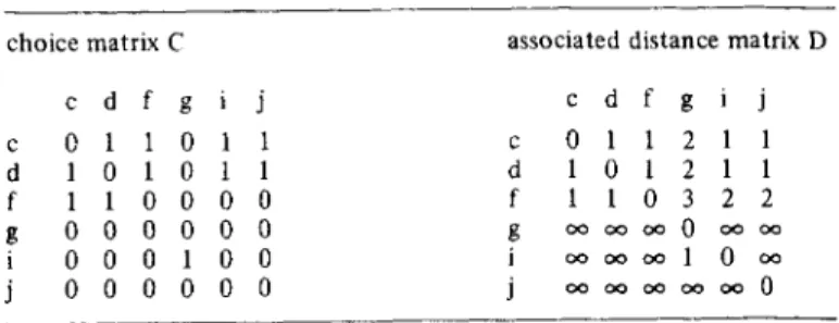
Considering the digraph as per Fig. 1 associated with the choice matrix C of Tab. 1 it may be seen, that person g, e.g., is in direct contact with person i. Though g did not directly choose c and f, for instance, both of them are reachable for g through intermediary links (i, and, i and c, respec
tively). Graph theory does make use of this fact
to define a measure of graph theoretical distance, which simply is the length of the shortest path between two points, or the number of steps of a chain from i to j. Instead of counting the number of steps, the matrix D of distances is achieved by raising C to successively higher powers (max.
N—1) and defining
( min {k: cH> 0 } d i j -
[ °°, if cjj = 0 for k= 1, N—1
k k
where cy refers to the i,j-th entry of C , and djj: =0. From the resulting distance matrix D (see Tab. 1) two facts are obvious:
1) the matrix is nonsymmetric. Possibilities of handling nonsymmetric matrices will be dis
cussed in the Appendix, and,
2) in this example a relatively high number of en
tries has a value °°, which may not be true for empirical data. However, the consequence is that a numerical analysis is impossible for the whole group, i.e., only connected parts of a network may be analyzed. This clearly is a dis
advantage adherent to the path distance mea
sure of proximity as compared with other measures that provide an index for each pair of a group.
FIG. 1: Graph associated with choise matrix C
TAB. 1: Artificial choice matrix C and associated distance matrix D choice matrix C
c d f g i j
c 0 1 1 0 1 1
d I 0 1 0 1 1
f 1 1 0 0 0 0
g 0 0 0 0 0 0
i 0 0 0 1 0 0
j 0 0 0 0 0 0
associated distance matrix D
c d f g i j
c 0 1 1 2 1 1
d 1 0 1 2 1 1
f 1 1 0 3 2 2
g O O O O O O 0 o o o o
i O O O O O O 1 0 O O
oo oo oo
192 Zeitschrift für Soziologie, Jg. 6, Heft 2, April 1977, S. 189-202 The artificial data used here make clear further
more, that different persons can reach others via different paths (cf. paths g-i-c-f and g-i-d-f)- In conceiving a measure of proximity that adequate
ly maps processes of diffusion, this point should be realized. Therefore, “the measure should be constructed so that: (a) the greater the number of paths joining two individuals, the more proxi
mate they are defined to be; (b) the longer the paths joining the two, the less proximate they are defined to be” (ALBA 1975: 17). Both of these criteria are satisfied in measures developed by HUBBELL (1965) and ALBA and KADUSHIN (1970), using all powers of the weighted choice matrix (cf. measures 12 to 14 in the Appendix).
Originally, these measures go back to KATZ (1953), who proposed this concept in developing a refined status index. One disadvantage specific to these measures is what has been called the problem of “redundant chains” by LUCE and PERRY (1949) or “doubling back” by COLEMAN (1964), i.e., the same element may be part of a chain more than once (cf. chain i-c-d-f-c-d in Fig. 1). This results in counting the same connec
tions more than once. COLEMAN (1964) has de
vised an approximate method for eliminating such redundant chains. His method, however, errs in the opposite direction in that it counts too few chains. Another point to be mentioned is, that the weights used in computing measures of dyadic association are not free of arbitrariness. But, ac
cording to HUBBELL (1965), different values will not substantially alter the order of appea- rence of cliques. In fact, if one chooses the sum of each persons weights to be .5 as proposed by HUBBELL, further computations are based on a clear rationale, and a solution of the mathema
tical system will exist, provided each person has given at least one choice.
Comparing the characteristics of a diffusion pro
cess with those of a process o f social cohesion, ALBA (1975) comes to the conclusion, that all of the measures just mentioned do not apply to a cohesion process, since “criteria for a measure of social proximity in a diffusion process result from the independence of transmission probabilities”
(ALBA 1975: 19). In a cohesion process, on the other hand, “transmission across any one link is not statistically independent of transmission across other links” (ALBA 1975: 18). A family of SIMMEL-measures (referring to SIMMEL’s (1908) contributions to the theory o f informal
social groups) has been constructed therefore, starting from the following basic ideas:
1) each person has an interpersonal environment (i.e., those persons i is in contact with), and, 2) the overlap of interpersonal environments common to persons i and j may serve as an indicator of the strength of cohesive forces between both of them.
Some further assumptions in finally defining these measures are:
1) relationships are symmetric,
2) persons may be linked directly or indirectly, but
3) the number of indirect links should be limited to some specific distance “n”, i.e., the “social neighborhood of radius n ”, depending on pro
perties of the network or kind of communica
tion under consideration.
The three SIMMEL-measures finally defined are different in the way they are normalized. Common to all of them is the term in the numerator, i.e., the number of persons being within the social neighborhood of both i and j at radius “n” . In the case of SIMMELl the maximum number of elements in the smaller of the two social neigh
borhoods is taken to be the denominator. SIM- MEL2 (cf. measure 16 in the Appendix) uses the number of people in the combined social neighbor
hoods of i and j, and, SIMMEL3, finally, takes the number of people in the network (ALBA 1975;
ALBA and GUTMANN 1972, 1974).
ALBA (1975) argues, that the SIMMEL-measures have the following advantages in comparison to those measures based on the weighted choice matrix:
1) there is a sound theoretical basis that makes these measures suitable especially to quantify processes of cohesion, and,
2) due to the mathematical operations necessary, the SIMMEL-measures are considerably faster to compute, especially in the case of large groups.
Comparing the features of these indices with some
R. Langeheine: Measures of Social Proximity and their Use in Sociometric Research 193 others on data provided by LAUMANN and
PAPPI (1973), SIMMEL2 turned out to be the best predictor of social distance between indivi
duals as judged from several criteria (ALBA 1975).
Nevertheless, it should be kept in mind, that the distance used in determining the number of indi
viduals within each person’s neighborhood is arbi
trary, as mentioned too by ALBA (1975). May
be, results turn out to be different to a more or less degree whether “n ” is set to 2 or 3, for in
stance. A further disadvantage may be seen in the fact, that only symmetric relationships are ana
lyzed. If the aim of an analysis, e.g., is to construct a new seating arrangement for a school class, it seems quite necessary to take into consideration TAB. 2: G-L SSA-I of 36 Proximity Measures
negative reationships as well. Another difficulty will arise with isolates in this specific case, since one cannot simply drop them from the analysis.
Normally, isolates at least choose anyone of the network. But this relationship will be converted to be nonexisting if only symmetric ones are used.
4. Proximity of proximity measures Throughout section 3 it has been argued that different measures of proximity are expected to map different aspects of a network. That is, these measures should be more or less correlated, de
pending on the concepts used to define two mea-
Variable Data Dimension
Type 1 2
1 chosen scalar products 2 chooser scalar products 3 chosen euclidian distances 4 chooser euclidian distances 5 chosen/chooser sym. euclid. dist.
6 chosen common elements 7 chooser common elements 8 HUBBELL minimum 9 HUBBELL arithmetic mean 10 HUBBELL geometric mean 11 chosen scalar products 12 chooser scalar products 13 chosen euclidian distances 14 chooser euclidian distances 15 chosen/chooser sym. euclid. dist.
16 chosen common elements 17 chooser common elements 18 chosen G-index
19 chooser G-index 20 HUBBELL minimum 21 HUBBELL arithmetic mean 22 HUBBELL geometric mean 23 chosen scalar products 24 chooser scalar products 25 chosen euclidian distances 26 chooser euclidian distances 27 chosen/chooser sym. euclid. dist.
28 chosen common elements 29 chooser common elements 30 chosen G-index
31 chooser G-index 32 HUBBELL minimum 33 HUBBELL arithmetic mean 34 HUBBELL geometric mean 35 SIMMEL2 “ n”=3
36 SIMMEL2 “ n”=3
All 0.812 -0.061
,,
0.681 -0.846,,
-1.000 0.031,,
-0.704 0.524,,
-0.893 0.262,,
0.748 -0.139,,
0.855 -0.764,,
0.588 -0.694,,
0.651 -0.597,,
0.651 -0.5930/1 0.276 -0.762
,,
0.377 -1.000,,
-0.866 -0.494,,
-0.753 0.308-0.915 -0.221
0.870 0.387
1.000 -0.356
0.859 0.395
>> 0.862 0.387
0.516 -0.530
,,
0.549 -0.6890.524 -0.569
MC 0.331 -0.817
0.331 -0.798 -0.770 -0.467 -0.773 -0.472 -0.836 -0.374
0.879 0.541
0.875 0.541
t 0.868 0.540
0.857 0.537
0.598 -0.368 0.545 -0.435 0.561 -0.430 0.438 -0.780
>> 0.414 -0.751
194 Zeitschrift für Soziologie, Jg. 6, Heft 2, April 1977, S. 189-202 sures. Relationships between measures may be
examined either “through a priori mathematical means” or by “a posteriori. .. determining their intercorrelations in an empirical situation”. Since the first approach is quite difficult “because of .. . complicated definitions” (ALBA 1975: 34) the a posteriori approach is used here (cf. LANGE- HEINE et al., 1975, for discussion of this problem within individual index analysis, another topic in sociometry). The strategy is nearly identical to that applied by ALBA (1975).
Starting from a 26 by 26 choice matrix of data type —1/0/+1 (students, choice criterion: seat mate, cf. LANGEHEINE et al. (1975)) as many proximity measures as possible are computed using
a) —1/0/+1 data, full information (labeled ALL from now),
b) 0/1 data, —1 set to 0 (labeled 0/1), and c) 0/1 data, mutual choices retained only
(labeled MC).
Thus, as well relationships between different measures may be examined (starting from same data) as relationships between same measures (starting from different data). The 36 variables used are listed in Tab. 2
The first step of the analysis was to compute these 36 proximity matrices. In order to examine the similarity of these matrices they have been correlated (product-moment) using as a unit for correlation between two matrices the respective proximity values of a pair of persons. That is, cor
relations are performed overN(N—1)/2 = 325 pairs of persons of each group. The resulting correlation matrix has been submitted to the G—L SSA—I
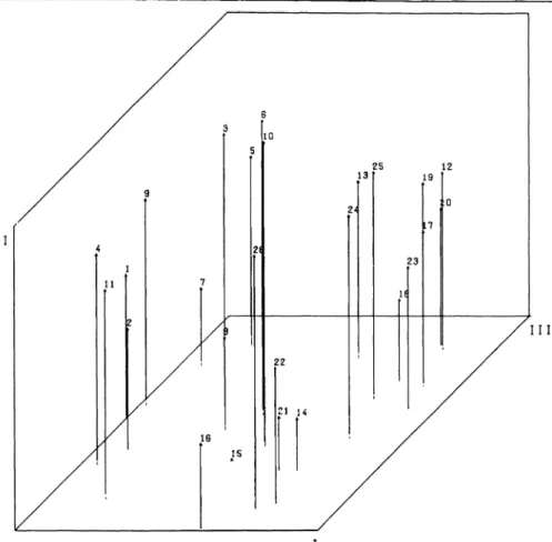
TAB. 3: Fit of 2 -4 dimensional SSA-I solutions 36 proximity measures
nonmetric multidimensional scaling routine (LINGOES 1965, 1973). As can be seen from Tab. 3, the fit is sufficient in favor of the 2-di
mensional solution, though there is an improve
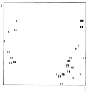
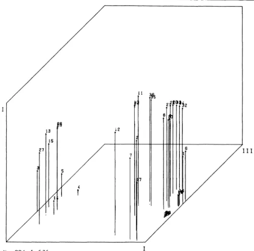
ment in fit with 3 dimensions. Therefore, both the 2- and 3-dimensional solution are presented in Figs. 2 and 3, respectively.
FIG. 2: 2-dim. SSA-I of 36 prox. meas.
Clearly, the first dimension separates euclidian distances from the rest of the measures. As to the second dimension, it may be labeled “chosen vs.
chooser ’. There is a regular pattern for those variables available for both chosen and chooser in that (cf. 2-dimensional solution) chosen measures are found more on top of the space, whereas chooser measures lie more at the bottom (vari
ables 1 vs. 2, 6 vs. 7, 11 vs. 12, 16 vs. 17). The opposed direction for euclidian distance measures is in line with this (variables 3,13 vs. 4,14). It may be noted, that some of the variables should have been discarded from the analysis since there is a chosen/chooser 1.0 correlation with MC-data, naturally.
Dimension Iterations
G-L coefficient of alienation
Kruskal’s stress
2 55 .111 .099
3 63 .067 .061
4 45 .046 0.41
Some specific results are more interesting, how
ever. First, it can be seen, that the proposal of symmetrizing nonsymmetric matrices (simpli
fied LINGOES approach) will yield measures, that lie about in between the respective chosen and chooser measures (variables 5,15). This ap
proach might be useful too with other measures
R. Langeheine: Measures of Social Proximity and their Use in Sociometric Research 195
FIG. 3: 3-dim. SSA-I of 36 prox. meas.
where information is at hand for both chosen and chooser and the interest is in a combination of both. Second, all of the HUBBELL measures are very close to each other, irrespective of whe
ther the minimum, arithmetic mean or geometric mean is used (variables 8,9,10; 20,21,22; 32,33, 34) and irrespective of information retained with raw data (ALL, 0/1, MC). Thus, it might indeed suffice to perform an analysis with the symmetric choice matrix only. This would allow a more par
simonious technique in gathering data. Third, as to SIMMEL2, according to this network it really makes no difference whether one decides for a distance of “n” = 2 or 3 to determine individual i’s social neighborhood (variables 35 and 36).
Forth, and this seems to be a bit surprising, SIMMEL2 turns out to be most close to MC and 0/1 scalar products (variables 23, 24, 11). This clearly is in conflict with properties assigned to the respective measures (Bogardus- vs. Sorokin-
type). If one examines, however, formulas accor
ding to which SIMMEL2 is computed, one will reveal, that this result is not that unexpected. In
deed, the essential term in the final SIMMEL2 formula is Sjj, which, put in matrix form, is R’R, where R is the reachability matrix (cf. Appendix).
R ’R differs from C’C only in that successive powers are utilized. Thus, sy is the degree of simi
larity in reachability pattern for persons i and j.
Sixth, it may be noted, that scalar products and common elements are relatively close to each other in case of ALL data (variables 1,6; 2,7) but not so with 0/1 and MC data. Therefore, with these measures, it makes quite a difference how much information is retained from the original choice matrix. Seventh, finally, the G-indices (variables 18, 19, 30, 31) are relatively indepen
dent of the other measures. This is due to the fact, that the strength of a relationship between persons i and j is essentially determined by 0,0
196 Zeitschrift für Soziologie, Jg. 6, Heft 2, April 1977, S. 189-202 correspondences, i.e., rejections in case of 0/1
data and even more with MC data.
The question to be raised now is: How general are these results? So far, no conclusive answer can be given, since only a single network has been analyzed. This study is exploratory in character, therefore. Further studies have to be performed using a larger number of networks. Only then an answer can be given to whether there is a regular and generalizable pattern for a set of sociometric proximity measures.
5. Identification o f cliques by dimensional analysis
The final goal in computing measures of social proximity is to submit these to some sort of ana
lysis in order to detect cliques. Different techni
ques have been proposed, among others cluster analysis (ALBA and GUTMANN 1972, 1974;
BOCK and HUSAIN 1950; HUBBELL 1965;
PEAY 1974, 1975), factor analysis (BEATON 1966; BOCK and HUSAIN 1952;MacRAE 1960;
WRIGHT and EVITTS 1961) and multidimen
sional scaling (ALBA and GUTMANN 1972, 1974; COLEMAN 1970; GLEASON 1969;
TOWNES 1969). Comparative studies using these and other techniques have been performed by NOSANCHUK (1963) and LANKFORD (1974).
LANKFORD (1974: 289) has pointed out that the factor analytic approach as well as multidi
mensional scaling have several advantages:
“ 1) it employs the matrix as a whole (not as seperate rows and columns)” (vs. rearranging the whole matrix), and
“2) the position of an individual in relation to all the subgroups of cliques may be describ
ed (overlapping and isolates possible)” . According to McFARLAND and BROWN (1973), however, we must assume, that the proximity measures presented in this paper do not satisfy the properties of metrics. Nonmetric multidimensio
nal scaling is the method of choice, therefore, constructing “a dimensional representation whose dimensions are interval scales, from only the rank order of the interpoint distances” (McFARLAND and BROWN 1973: 243).
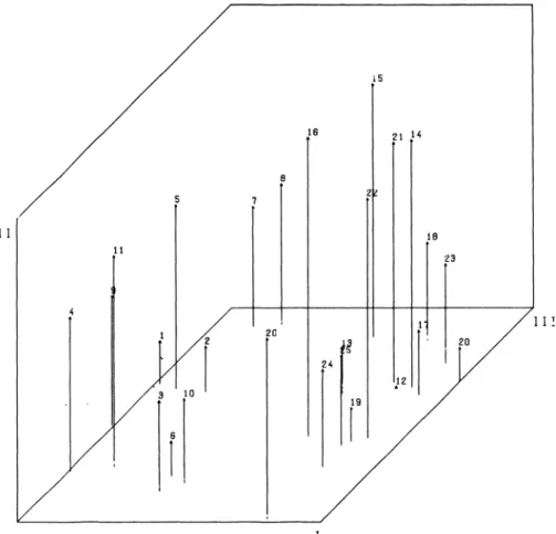
Two of such analyses will be reported here using a) the HUBBELL minimum measure and b) the HUBBELL geometric mean measure (ALL data used are those from the previous section).
Remembering the second argument given by LANKFORD it is proposed to submit the proxi
mity matrix to a nonmetric multidimensional sca
ling analysis and not to the partitioning technique applied by HUBBELL (1965).
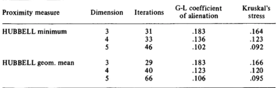
Both of the matrices have been run through the G -L S S A -I (LINGOES 1965, 1973). Solutions have been obtained from 3 to 5 dimensions. As judged from the fit measures (cf. Tab. 4), 4-di
mensional solutions are acceptable. Only 3-dimen
sional solutions are presented in Figs. 4 and 5, however.
According to the results from the previous sec
tion we would expect the solutions to be relative
ly similar. Comparison by visual inspection will confirm this. Nevertheless, determining which cliques are present is not quite easy even from the 3-dimensional representations. It is proposed
TAB. 4: Fit of 3 -5 dimensional SSA-I solutions. Proximity measures: HUBBELL minimum and HUBBELL geo
metric mean
Proximity measure Dimension Iterations G-L coefficient of alienation
Kruskal’s stress
HUBBELL minimum 3 31 .183 .164
4 33 .136 .123
5 46 .102 .092
HUBBELL geom. mean 3 29 .183 .166
4 40 .123 .120
5 66 .106 .095
R. Langeheine: Measures of Social Proximity and their Use in Sociometric Research 197
FIG. 4: 3-dimensional SSA-I solution HUBBELL minimum
therefore, to apply some clustering procedure to the SSA—I solutions in order to get interpretative support. The procedure used here is the hierarchi
cal MAXMIN clustering (LINGOES 1968). Accor
ding to the statistics provided by the program, one can realize a maximum mean (inter-) cluster distance for both HUBBELL minimum and geo
metric mean entering at level 4 and 5, respective
ly. Therefore, decision in favor of 3 cliques, 1 pair and 2 isolates seems to be optimal for HUBBELL minimum (level 3, cf. Tab. 5). In the case of HUB
BELL geometric mean one should decide for 5 cliques and 2 isolates (level 4, cf. Tab. 5). Since cluster analysis does not provide a unique solution, however, final decision in favor of any partitio
ning may be based on extra-statistical considera
tions, such as number of clusters desired, meaning
fulness etc. (LINGOES 1968). 3-dimensional MAXMIN solutions are reported only, since minor changes in clique structure resulted from cluster
ing in 4 dimesnions. Thus, the main differences between HUBBELL minimum and geometric mean solutions are as follows: First, HUBBELL geometric mean does more clearly seperate boys (1—11) and girls (12—26). At level 7 there is each a boy and a girl clique, a phenomenon well known in sociometry as “sex cleavage” (cf. dimension I).
In the HUBBELL minimum solution 3 boys (3, 6, 10) are members of the girl clique at the final le
vel. In fact, these 3 are the only boys having mu
tual choices with girls (19, 24, 25). Second, girl 26 is an outsider with no choices received. This is more clearly reflected by HUBBELL geometric mean. However, these results are not sufficient to support the hypothesis, that stronger cohesive forces will be reflected by the HUBBELL geo
metric mean measure as compared with the mini
mum measure.
The reader familiar with techniques of dimensio-
198 Zeitschrift für Soziologie, Jg. 6, Heft 2, April 1977, S. 189-202
FIG. 5: 3-dimensionai SSA-I solution HUBBELL geometric mean
nal analysis will probably expect some specifica
tions of the latent characteristics underlying the dimensions extracted, that is: According to what characteristics are members of one clique more proximate or less distant to each other than those of another clique? No such information is avai
lable from the proximity data. Therefore, the analysis performed is purely ‘internal’ (SHEPARD
1972), since the aim is to reveal the structure of the network. As to the latent characteristics these may be identified by relating the spatial represen
tation to ‘external’ variables. Dimension I, e.g., can be clearly associated with sex, but no answer can be given here as to the other dimensions, since further external variables are not available.
Appendix: MSP — A FORTRAN-IV program computing different measures of social proximity
The program takes both data of type 0/1 and
—1/0/+1 as input. If the concept underlying a specific measure allows for 0/1 or symmetric data only, transformation will be performed automati
cally. In addition, an option is provided to 1) leave input data unchanged, or, 2) set -1 in input data to 0, or,
3) retain mutual (symmetric) choices only.
Consequently, different sources of information may be used to examine a network, or, the same basic data may be started with to compare a net
work using, e.g., the HUBBELL and SIMMEL measures.
R. Langeheine: Measures of Social Proximity and their Use in Sociometric Research 199 TAB. 5: MAXMIN cluster analysis of 3-dimensional SSA-I solutions
Proximity persons level mean current
measure dist. criterion
0 0 0 0 0 0 1 0 0 0 1 2 1 2 2 1 1 1 1 2 2 1 1 1 2 2 7 8 1 2 9 4 1 5 3 6 0 6 4 1 2 6 5 7 2 0 3 8 3 9 4 5 g e o m e t r i c ---
mean ---
1 1
2 1
3 1
4 1
5 1
6 1
7 1
.352 .476
.390 .595
.423 .714
.444 .833
.451 .952
.434 1.071
.409 1.301
0 0 0 0 0 0 1 0 0 0 1 2 1 2 2 1 1 1 1 2 2 1 1 1 2 2 7 8 1 2 9 4 1 5 3 6 0 6 4 1 2 6 5 7 2 0 3 9 8 3 4 5
minimum 1 1.303 .452
2 1.342 .565
3 1.354 .678
4 1.424 1.017
5 1.339 1.243
the respective level mean dist.: mean inter-cluster distance entering at
current criterion: radius defined at the respective level
$: note change in position
In case of the Sorokin-type similarity measures each a column (chooser) or a row (chosen) solu
tion is available optionally, the resulting matrices of which are identical for symmetric data only.
Nonsymmetric proximity matrices will normally result with graph theoretical distances and the HUBBELL index. Different possibilities of de
fining symmetric proximity measures are dealt with when listing the measures provided by the program. Starting with the choice matrix C, where cü: =0 by definition and columns=chooser and rows=chosen,these measures are:
1) chosen mean scalar products: X = ^ CC 2) chooser mean scalar products: Y = ^ C’C 3) chosen euclidian distances:
xij = ^ J / cik- cjk) 2 ) 1/2
4) chooser euclidian distances:
yi J - R <! , (ck i - ‘ kj)2)1/2
5) chosen/chooser symmetrized euclidian distances:
N
z r kV x ik xj k H y w V ’
where X and Y are chosen and chooser eucli
dian distances. A more refined approach has been originally proposed by LINGOES within the Guttman-Lingoes nonmetric program series as an alternative to averaging the corresponding cells of a nonsymmetric matrix (cf. steps of the analysis in LINGOES (1973: 86—87)). Since distance axioms do not allow negative distances, the lowest negative value will be added to all coefficients to make them greater/equal zero, if an entry of the resulting matrix Z turns out to be less zero.
6) chosen common elements product moment 1 N
correlation: x4j = - j bijk),
where by :=1 if cik=Cjk, otherwise by:=0 by definition.
7) chooser common elements product moment
200 Zeitschrift für Soziologie, Jg. 6, Heft 2, April 1977, S. 189-202
correlation: = I b.jk),
where by: = 1 if c ^ p c ^ , otherwise b y :=0 by definition.
8) chosen Phi-Pearson, and, 9) chooser Phi-Pearson,
both of which are computed for 0/1 data only according to formula:
((a+b) (c+d) (a+c) (b+d))*^
where a,b,c and d refer to the frequencies f( 1,1), f(l,0 ), f(0 ,l) and f(0,0), counted for rows and columns of C, respectively. How
ever, if the requirements in computing 4> are not met, Yates’ correction or even other co
efficients may be more adequate (cf. LIE- NERT 1973).
10) chosen G-Index, and 11) chooser G-Index
G-indices, too, are computed for 0/1 data only according to formula:
= (a+d) - (b+g)
Sij N
where I is the identity matrix. Correspon
ding to each pair of group members i,j there are two entries in Y, i.e., y-. and y.-, where normally. HUBBELL pro
posed to use Jthe smaller of these values my = min(yy,yjj) in detecting cliques, since my does indicate the lower bound of association between both of them.
It is proposed here, however, to make use of the full information available by com
puting either arithmetic or geometric means for each pair i,j. In the case of geo
metric means, especially, it is assumed, that a relationship is stronger if y-. and y~
are more equal each other (cf., Yy” Yji=
will result in both .4 for arithmetic and geometric mean. With y~=.6 and y.*=.2, on the other hand, the resulting values are .4 and .35, respectively). The following three HUBBELL measures are therefore offered by the program:
12) my = minCyjj, yjj), or yii + yii 13) rnjj = —=2— - , o r , 14) my = (yy yji)1^2- using frequencies a to d as stated above.
12-14) HUBBELL indices of dyadic association.
Basic to three different measures obtainable from the HUBBELL input—output model (HUBBELL 1965) are the following steps in computation:
a) normalize the choice matrix C to obtain the weighted choice matrix W, where
If, in the latter case, any one yy turns out to be negative, all values of Y are reset to yjj = yy + I min(yij) | + .001 .
15) Graph theoretical distances.
As to computation of the distance matrix see section 3.2. The full series of up to N - l powers is used. If two persons are not reach
able, their entry is set to N.
Wy = cij
N 2 2
k = l ckj
b) obtain Y, the matrix of association indi
ces searched for, by using all powers of W, i.e.,
Y = I+W+W2+W3+ . . .
= ( I - W T 1,
16) SIMMEL2.
This measure may be computed for a speci
fied value of “n ” , the distance allowed to de
fine the social neighborhood of radius “n”
around person i. That is, the reachability ma
trix R is defined first for i ^ j [ 0, if Cy = 0 for k= 1 ,n ry : = j
I 1 otherwise
R. Langeheine: Measures of Social Proximity and their Use in Sociometric Research 201 and rjj: = 0. Then, the intersection of the
neighborhoods of any two persons i and j is simply the sum of persons both i and j reach in common:
N
sij = k? ! rikrjk '
Aditionally, both i and j are within this inter
section if they both reach each other. Hence, if rij=rji =^= 0, then ssjj: = 2, otherwise ssy: = 0 by definition.
The term (sy+ssy) is divided by the number of persons in the combined social neighbor
hoods of i and j. Number of persons reach
able by i and j, respectively, are nr.
N i ^ rik 1 k= 1 lk
N and nr. = 2 r-v ,
J k= 1 Jic
^o that, finally SIMMEL2;;
S-- + SS-.
1J 1J 1J nri + nrj ~~ sij
The program is available from the author at a charge covering costs.
References
ALBA, R.D., 1975: “The intersection of social circles” : A new measure of social proximity in networks.
Paper presented at the 1975 American Sociological Association meetings in San Francisco.
ALBA, R.D., M.P. GUTMANN, 1972: SOCK: A socio- metric analysis system. Behavioral Science 17, 326- 327.
ALBA, R.D., M.P. GUTMANN, 1974: SOCK: A socio
metric analysis system. Bureau of Applied Social Research, Columbia University.
ALBA, R.D., C. KADUSHIN, 1970: Sociometric clique identification. Bureau of Applied Social Research, Columbia University.
BEATON, A., 1966: An inter-battery factor analytic approach to clique analysis. Sociometry 29, 135-145.
BOCK, R.D., S.Z. HUSAIN, 1950: An adaptation of Holzinger’s B-coefficient for the analysis of socio
metric data. Sociometry 13, 146-153.
BOCK, R.D., S.Z. HUSAIN, 1952: Factors of the tele:
A preliminary report. Sociometry 15, 206-219.
BOGARDUS, E.S., 1925: Measuring social distance.
Journal of Applied Sociology 9, 299-308.
BOGARDUS, E.S., 1933: A social distance scale. Socio
logy and Social Research 17, 265-271.
COLEMAN, J.S., 1964: Introduction to mathematical sociology. New York: The Free Press.
COLEMAN, J.S., 1970: Clustering in N dimensions by use of a system of forces. Journal of Mathematical Sociology 1, 1-47.
COOMBS, C.H., R.M. DAWES, A. TVERSKY, 1970:
Mathematical Psychology. Englewood Cliffs:
Prentice-Hall.
GLEASON, T.C., 1969: Multidimensional scaling of sociometric data. Doctoral dissertation. Ann Arbor:
The University of Michigan.
HARARY, F., R.Z. NORMAN, D. CARTWRIGHT, 1965: Structural models: An introduction to the theory of directed graphs. New York: J. Wiley and Sons.
HUBBELL, C.H., 1965: An input-output approach to clique identification. Sociometry 28, 377-399.
KATZ, L., 1953: A new status index derived from sociometric analysis. Psychometrika 18, 39-43.
LANGEHEINE, R., E. HÖRNER, K. KUCHNER, M.
VOGES, 1975: Anwendung soziometrischer Techni
ken zur Erstellung einer neuen Sitzordnung in Schul
klassen. Ein Beitrag zur Hochschuldidaktik. Kiel:
C.A.U.S.A. 1. Christian-Albrechts-Universität Sozio
logische Arbeitsberichte.
LANKFORD, P.M., 1974: Comparative analysis of clique identification methods. Sociometry 37, 287-305.
LAUMANN, E.O., F.U. PAPPI, 1973: New directions in the study of community elites. American Sociologi
cal Review 38, 212-229.
LIENERT, G.A., 1973: Verteilungsfreie Methoden in der Biostatistik. Meisenheim: A. Hain.
LINGOES, J.C., 1965: An IBM-7090 program for Guttman-Lingoes smallest space analysis-I. Behav
ioral Science 10, 183-184.
LINGOES, J.C., Ä968: The multivariate analysis of qualitative data. Multivariate Behavioral Research 3,61-94.
LINGOES, J.C., 1970: An IBM 360/67 program for Guttman-Lingoes smallest space analysis -PI. Be
havioral Science 15, 536-540.
LINGOES, J.C., 1973: The Guttman-Lingoes nonmetric program series. Ann Arbor: Mathesis Press.
LUCE, R.D., 1950: Connectivity and generalized cliques in sociometric group structure. Psychome
trika 15, 169-190.
LUCE, R.D., A.D. PERRY, 1949: A method of matrix analysis of group structure. Psychometrika 14, 9 5 - 116.
McFARLAND, D.D., D J. BROWN, 1973: Social dis
tance as a metric: A systematic introduction to smallest space analysis. In: Laumann, E. O.: Bonds of pluralism: The form and substance of urban social networks. New York: J. Wiley and Sons.
MacRAE, D. jr., 1960: Direct factor analysis of socio
metric data. Sociometry 23, 361-371.
NOSANCHUK, T.A., 1963: A comparison of several sociometric partitioning techniques. Sociometry 26, 112-124.
PEAY, E.R., 1974: Hierarchical clique structures. Socio
metry 37, 54-65.
PEAY, E.R., 1975: Nonmetric grouping: Clustersand cliques. Psychometrika 40, 297-313.
SHEPARD, R.N., 1972: A taxonomy of some principal types of data and of multidimensional methods for
202 Zeitschrift für Soziologie, Jg. 6, Heft 2, April 1977, S. 189-202 their analysis. In: SHEPARD, R.N., A.K. ROMNEY,
S.B. NERLOVE (eds.): Multidimensional scaling, Vol. I. New York: Seminar Press.
SIMMEL, G., 1908: Soziologie. Leipzig: Duncker und Humblot.
SOROKIN, P.A., 1927: Social mobility. (Retitled
“Social and cultural mobility” and reprinted in 1959).
New York: The Free Press.
TOWNES, B.D., 1969: Nonmetric multidimensional scaling of sociometric data. Doctoral dissertation.
Washington: The University of Washington.
TUCKER, L.R., 1958: An inter-battery method of fac
tor analysis. Psychometrika 23, 111-136.
WRIGHT, B., M.S. EVITTS, 1961: Direct factor analysis in sociometry. Sociometry 24, 82-98.
Anschrift des Verfassers:
Dipl.- Psych. ROLF LANGEHEINE Ahlmannstr. 15
2300 Kiel 1