To be published by SIAM in 2000.

(1)

MATLAB Guide1

Desmond J. Higham and Nicholas J. Higham Version of June 27, 2000

To be published by SIAM in 2000.

Not for distribution

1c D. J. Higham and N. J. Higham, 2000

(2)

(3)

(4)

List of Figures

1.1 MATLAB desktop at start of tutorial. . . 2

1.2 Basic 2D picture produced by^plot. . . 8

1.3 Histogram produced by^hist. . . 8

1.4 Growth of a random Fibonacci sequence. . . 9

1.5 Plot produced by^collatz.m. . . 11

1.6 Plot produced by^collbar.m. . . 13

1.7 Mandelbrot set approximation produced by^mandel.m. . . 14

1.8 Phase plane plot from^ode45. . . 15

1.9 Removal process for the Sierpinski gasket. . . 17

1.10 Level 5 Sierpinski gasket approximation from^gasket.m. . . 17

1.11 Sierpinski gasket approximation from^barnsley.m. . . 18

1.12 3D picture produced by^sweep.m. . . 19

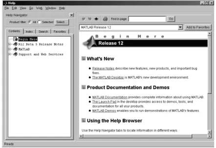
2.1 Help Browser. . . 26

2.2 Workspace Browser. . . 28

2.3 Array Editor. . . 28

7.1 Histogram produced by^rouldist. . . 69

7.2 MATLAB Editor/Debugger. . . 74

8.1 Simplex-y plots. Left: default. Right: nondefault. . . 78

8.2 Two nondefaultx-y plots. . . 79

8.3 ^loglogexample. . . 80

8.4 Using^{axis off}. . . 81

8.5 Use of^ylim(right) to change automatic (left)y-axis limits. . . 82

8.6 Epicycloid example. . . 83

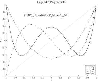
8.7 Legendre polynomial example, using^legend. . . 84

8.8 Bezier curve and control polygon. . . 86

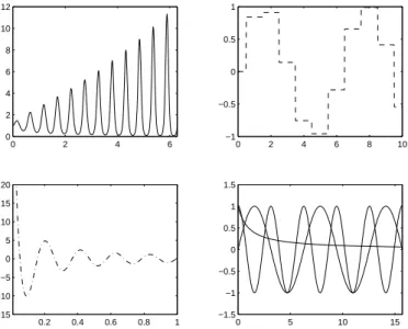
8.9 Example with^subplotand^fplot. . . 87

8.10 First 5 (upper) and 35 (lower) Chebyshev polynomials, plotted using fplotand^chebyin Listing 7.4. . . 88

8.11 Irregular grid of plots produced with^subplot. . . 89

8.12 3D plot created with^plot3. . . 90

8.13 Contour plots with^ezcontour(upper) and ^contour(lower). . . 91

8.14 Contour plot labelled using^clabel. . . 92

8.15 Surface plots with^meshand^meshc. . . 93

8.16 Surface plots with^surf,^surfcand ^waterfall. . . 94

8.17 3D view of a 2D plot. . . 95

8.18 Fractal landscape views. . . 97

8.19 ^surfcplot of matrix containing NaNs. . . 98

8.20 Riemann surface forz¹⁼³. . . 98 xi

(9)

xii List of Figures

8.21 2D bar plots. . . 100

8.22 3D bar plots. . . 101

8.23 Histograms produced with^hist. . . 102

8.24 Pie charts. . . 103

8.25 Area graphs. . . 103

8.26 From the 1964 Gatlinburg Conference on Numerical Algebra. . . 105

10.1 Koch curves created with function^koch. . . 133

10.2 Koch snowake created with function^koch. . . 133

11.1 Left: least squares polynomial t of degree 3. Right: cubic spline. Data is from 1=(x+ (1^;x)²). . . 137

11.2 Interpolating a sine curve using^interp1. . . 139

11.3 Interpolation with^griddata. . . 140

11.4 Plot produced byezplot('x-tan(x)',[-pi,pi]), grid. . . 141

12.1 Integration of ^humpsfunction by^quad. . . 147

12.2 Fresnel spiral. . . 147

12.3 Scalar ODE example. . . 150

12.4 Pendulum phase plane solutions. . . 152

12.5 Rossler system phase space solutions. . . 153

12.6 Pursuit example. . . 155

12.7 Pursuit example, with capture. . . 156

12.8 Chemical reaction solutions. Left: ^ode45. Right: ^ode15s. . . 158

12.9 Zoom of chemical reaction solution from^ode45. . . 158

12.10 Sti ODE example, with Jacobian information supplied. . . 161

12.11 Water droplet BVP solved by^bvp4c. . . 165

12.12 Liquid crystal BVP solved by^bvp4c. . . 168

12.13 Skipping rope eigenvalue BVP solved by^bvp4c. . . 170

12.14 Black{Scholes solution with^pdepe. . . 174

12.15 Reaction-diusion system solution with^pdepe. . . 176

15.1 Wathen matrix (left) and its Cholesky factor (right). . . 193

15.2 Wathen matrix (left) and its Cholesky factor (right) with symmetric reverse Cuthill{McKee ordering. . . 193

15.3 Wathen matrix (left) and its Cholesky factor (right) with symmetric minimum degree ordering. . . 193

16.1 profile plotfor^membraneexample. . . 198

17.1 Hierarchical structure of Handle Graphics objects. . . 202

17.2 Left: original. Right: modied by^setcommands. . . 203

17.3 Straightforward use of ^subplot. . . 205

17.4 Modied version of Figure 17.3 postprocessed using Handle Graphics. 205 17.5 One frame from a movie. . . 208

17.6 Animated gure upon completion. . . 209

17.7 Default (upper) and modied (lower) settings. . . 210

17.8 Word frequency bar chart created by^wfreq. . . 212

17.9 Example with superimposed Axes created by script^garden. . . 214

17.10 Diagram created by^{sqrt ex}. . . 214

(10)

List of Figures xiii

18.1 cellplot(testmat). . . 225

19.1 ^taylortoolwindow. . . 234

20.1 Approximate Brownian path. . . 243

20.2 Numerical bifurcation diagram. . . 246

(11)

(12)

List of Tables

1 Versions of MATLAB. . . xx

2.1 ^10*exp(1)displayed in several output formats. . . 24

2.2 MATLAB directory structure (under Windows). . . 25

2.3 Command line editing keypresses. . . 27

2.4 Information and demonstrations. . . 29

4.1 Arithmetic operator precedence. . . 37

4.2 Elementary and special mathematical functions. . . 38

5.1 Elementary matrices. . . 40

5.2 Special matrices. . . 42

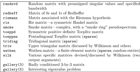
5.3 Matrices available through^gallery. . . 43

5.4 Matrices classied by property. . . 44

5.5 Elementary matrix and array operations. . . 47

5.6 Matrix manipulation functions. . . 51

5.7 Basic data analysis functions. . . 55

6.1 Selected logical^is*functions. . . 58

6.2 Operator precedence. . . 59

8.1 Options for the^plotcommand. . . 78

8.2 Some commands for controlling the axes. . . 81

8.3 Some of the TEX commands supported in text strings. . . 85

8.4 2D plotting functions. . . 89

8.5 3D plotting functions. . . 97

9.1 Iterative linear equation solvers. . . 122

12.1 MATLAB's ODE solvers. . . 160

18.1 Multidimensional array functions. . . 221

19.1 Calculus functions. . . 234

19.2 Linear algebra functions. . . 237

B.1 Application toolboxes marketed by The MathWorks. . . 259

xv

(13)

(14)

List of M-Files

1.1 Script M-le^rfib.m. . . 10

1.2 Script M-le^collatz.m. . . 11

1.3 Script M-le^collbar.m. . . 13

1.4 Script M-le^mandel.m. . . 14

1.5 Function M-le^lorenzde.m. . . 15

1.6 Script M-le^lrun.m. . . 15

1.7 Function M-le^gasket.m. . . 16

1.8 Script M-le^barnsley.m. . . 18

1.9 Script M-le^sweep.m. . . 19

7.1 Script^rouldist. . . 68

7.2 Function^maxentry. . . 70

7.3 Function^flogist. . . 70

7.4 Function^cheby. . . 71

7.5 Function^sqrtn. . . 72

7.6 Function^marks2. . . 73

8.1 Function^land. . . 95

10.1 Function^{fd deriv}. . . 127

10.2 Function^poly1err. . . 128

10.3 Function^companb. . . 130

10.4 Function^moments. . . 130

10.5 Function^koch. . . 132

12.1 Functions^fox2and ^events. . . 156

12.2 Function^rcd. . . 162

12.3 Function^lcrun. . . 167

12.4 Function^skiprun. . . 169

12.5 Function^bs. . . 173

12.6 Function^mbiol. . . 175

14.1 Script ^fibthat generates a runtime error. . . 184

16.1 Script ^ops. . . 199

17.1 Script ^wfreq. . . 212

17.2 Script ^gardento produce Figure 17.9. . . 213

17.3 Script ^{sqrt ex}. . . 215

20.1 Script^bif1. . . 245

20.2 Script^bif2. . . 246 xvii

(15)

(16)

Preface

MATLAB¹ is an interactive system for numerical computation. Numerical analyst Cleve Moler wrote the initial Fortran version of MATLAB in the late 1970s as a teaching aid. It became popular for both teaching and research and evolved into a commercial software package written in C. For many years now, MATLAB has been widely used in universities and industry.

MATLAB has several advantages over more traditional means of numerical computing (e.g., writing Fortran or C programs and calling numerical libraries):

It allows quick and easy coding in a very high-level language.

Data structures require minimal attention; in particular, arrays need not be declared before rst use.

An interactive interface allows rapid experimentation and easy debugging.

High-quality graphics and visualization facilities are available.

MATLAB M-les are completely portable across a wide range of platforms.

Toolboxes can be added to extend the system, giving, for example, specialized signal processing facilities and a symbolic manipulation capability.

A wide range of user-contributed M-les is freely available on the Internet.

Furthermore, MATLAB is a modern programming language and problem solving envi- ronment: it has sophisticated data structures, contains built-in debugging and prol- ing tools, and supports object-oriented programming. These factors make MATLAB an excellent language for teaching and a powerful tool for research and practical problem solving. Being interpreted, MATLAB inevitably suers some loss of e- ciency compared with compiled languages, but this can be mitigated by using the MATLAB Compiler or by linking to compiled Fortran or C code using MEX les.

This book has two purposes. First, it aims to give a lively introduction to the most popular features of MATLAB, covering all that most users will ever need to know.

We assume no prior knowledge of MATLAB, but the reader is expected to be familiar with the basics of programming and with the use of the operating system under which MATLAB is being run. We describe how and why to use MATLAB functions but do not explain the mathematical theory and algorithms underlying them; instead, references are given to the appropriate literature.

The second purpose of the book is to provide a compact reference for all MATLAB users. The scope of MATLAB has grown dramatically as the package has been devel- oped (see Table 1), and even experienced MATLAB users may be unaware of some of the functionality of the latest version. Indeed the documentation provided with

1MATLAB is a registered trademark of The MathWorks, Inc.

xix

(17)

xx Preface Table 1. Versions of MATLAB.

Year Version Notable features

1978 Classic MATLAB Original Fortran version.

1984 MATLAB 1 Rewritten in C.

1985 MATLAB 2 30% more commands and functions, typeset documentation.

1987 MATLAB 3 Faster interpreter, color graphics, high- resolution graphics hard copy.

1992 MATLAB 4 Sparse matrices, animation, visualization, user interface controls, debugger, Handle Graphics, Microsoft Windows support.

1997 MATLAB 5 Proler, object-oriented programming, multidimensional arrays, cell arrays, structures, more sparse linear algebra, new ordinary dierential equation solvers, browser-based help.

2000 MATLAB 6 MATLAB desktop including Help Browser, matrix computations based on LAPACK with optimized BLAS, function handles, ^eigs interface to ARPACK, boundary value problem and partial dierential equation solvers, graphics object transparency, Java support.

Handle Graphics is a registered trademark of The MathWorks, Inc.

MATLAB has grown to such an extent that the introductory Using MATLAB [56]

greatly exceeds this book in page length. Hence we believe that there is a need for a manual that is wide-ranging yet concise. We hope that our approach of focus- ing on the most important features of MATLAB, combined with the book's logical organization and detailed index, will make MATLAB Guide a useful reference.

The book is intended to be used by students, researchers and practitioners alike.

Our philosophy is to teach by giving informative examples rather than to treat every function comprehensively. Full documentation is available in MATLAB's online help and we pinpoint where to look for further details.

Our treatment includes many \hidden" or easily overlooked features of MATLAB and we provide a wealth of useful tips, covering such topics as customizing graphics, M-le style, code optimization and debugging.

The main subject omitted is object-oriented programming. Every MATLAB user benets, perhaps unknowingly, from its object-oriented nature, but we think that the typical user does not need to program in an object-oriented fashion. Other areas not covered include Graphical User Interface tools, MATLAB's Java interface, and some of the more advanced visualization features.

We have not included exercises; MATLAB is often taught in conjunction with particular subjects, and exercises are best tailored to the context.

(18)

Preface xxi We have been careful to show complete, undoctored MATLAB output and to test every piece of MATLAB code listed. The only editing we have done of output has been to break over-long lines that continued past our right margin|in these cases we have manually inserted the continuation periods \^..." at the line break.

MATLAB runs on several operating systems and we concentrate on features com- mon to all. We do not describe how to install or run MATLAB, or how to customize it|the manuals, available in both printed and online form, should be consulted for this system-specic information.

A Web page has been created for the book, at

http://www.siam.org/books/ot75

It includes

All the M-les used as examples in the book.

Updates relating to material in the book.

Links to various MATLAB-related Web resources.

What This Book Describes

This book describes MATLAB 6 (Release 12), although most of the examples work with at most minor modication in MATLAB 5.3 (Release 11). If you are not sure which version of MATLAB you are using type ^ver or ^version at the MATLAB prompt. The book is based on a prerelease version of MATLAB 6, and it is possible that some of what we say does not fully reect the release version; any corrections and additions will be posted on the Web site mentioned above.

All the output shown was generated on a Pentium III machine running MATLAB under Windows 98.

How This Book Is Organized

The book begins with a tutorial that provides a quick tour of MATLAB. The rest of the book is independent of the tutorial, so the tutorial can be skipped|for example, by readers already familiar with MATLAB.

The chapters are ordered so as to introduce topics in a logical fashion, with the minimum of forward references. A principal aim was to cover M-les and graphics as early as possible, subject to being able to provide meaningful examples. Later chapters contain material that is more advanced or less likely to be needed by the beginner.

Using the Book

Readers new to MATLAB should begin by working through the tutorial in Chapter 1.

Although it is designed to be read sequentially, with most chapters building on material from earlier ones, the book can be read in a nonsequential fashion by following cross-references and making use of the index. It is dicult to do serious MATLAB computation without a knowledge of arithmetic, matrices, the colon notation, oper- ators, ow control and M-les, so Chapters 4{7 contain information essential for all users.

Experienced MATLAB users who are upgrading from versions earlier than version 6 should refer to Appendix A, which lists some of the main changes in recent releases.

(19)

xxii Preface

Acknowledgments

We are grateful to a number of people who oered helpful advice and comments during the preparation of the book:

Penny Anderson, Christian Beardah, Tom Bryan, Brian Duy, Cleve Moler, Damian Packer, Harikrishna Patel, Larry Shampine, Francoise Tisseur, Nick Trefethen, Jack Williams.

Once again we enjoyed working with the SIAM sta, and we thank particularly Vickie Kearn, Michelle Montgomery, Deborah Poulson, Lois Sellers, Kelly Thomas, Marianne Will, and our copy editor, Beth Gallagher.

For those of you that have not experienced MATLAB, we would like to try to show you what everybody is excited about ...

The best way to appreciate PC-MATLAB is, of course, to try it yourself.

| JOHN LITTLE and CLEVE MOLER, A Preview of PC-MATLAB (1985) In teaching, writing and research, there is no greater clarier than a well-chosen example.

| CHARLES F. VAN LOAN, Using Examples to Build Computational Intuition (1995)

(20)

Chapter 1 A Brief Tutorial

The best way to learn MATLAB is by trying it yourself, and hence we begin with a whirlwind tour. Working through the examples below will give you a quick feel for the way that MATLAB operates and an appreciation of its power and exibility.

The tutorial is entirely independent of the rest of the book|all the MATLAB features introduced are discussed in greater detail in the subsequent chapters. Indeed, in order to keep this chapter brief, we have not explained all the functions used here.

You can use the index to nd out more about particular topics that interest you.

The tutorial contains commands for you to type at the command line. In the last part of the tutorial we give examples of script and function les|MATLAB's versions of programs and functions, subroutines, or procedures in other languages. These les are short, so you can type them in quickly. Alternatively, you can download them from the Web site mentioned in the preface on p. xxi. You should experiment as you proceed, keeping the following points in mind.

Upper and lower case characters are not equivalent (MATLAB is case sensitive).

Typing the name of a variable will cause MATLAB to display its current value.

A semicolon at the end of a command suppresses the screen output.

MATLAB uses both parentheses,⁽⁾, and square brackets,^[], and these are not interchangeable.

The up arrow and down arrow keys can be used to scroll through your previous commands. Also, an old command can be recalled by typing the rst few characters followed by up arrow.

You can type ^{help topic}to access online help on the command, function or symbol ^topic.

You can quit MATLAB by typing ^exitor^quit.

Having entered MATLAB, you should work through this tutorial by typing in the text that appears after the MATLAB prompt, ^>>, in the Command Window. After showing you what to type, we display the output that is produced. We begin with

>> a = [1 2 3]

a =

1 2 3

1

(21)

2 A Brief Tutorial

Figure 1.1. MATLAB desktop at start of tutorial.

This means that you are to type \a = [1 2 3]", after which you will see MATLAB's output \^{a =}" and \¹ ² ³" on separate lines separated by a blank line.

See Figure 1.1. (To save space we will subsequently omit blank lines in MATLAB's output. You can tell MATLAB to suppress blank lines by typingformat compact.) This example sets up a 1-by-3 array^a(a row vector). In the next example, semicolons separate the entries:

>> c = [4; 5; 6]

c = 4 5 6

A semicolon tells MATLAB to start a new row, so^cis 3-by-1 (a column vector). Now you can multiply the arrays^aand^c:

>> a*c ans =

32

Here, you performed an inner product: a 1-by-3 array multiplied into a 3-by-1 array.

MATLAB automatically assigned the result to the variable ^ans, which is short for answer. An alternative way to compute an inner product is with the^dotfunction:

>> dot(a,c) ans =

32

Inputs to MATLAB functions are specied after the function name and within parentheses. You may also form the outer product:

>> A = c*a

(22)

A Brief Tutorial 3

A =

4 8 12

5 10 15

6 12 18

Here, the answer is a 3-by-3 matrix that has been assigned to^A.

The product^a*ais not dened, since the dimensions are incompatible for matrix multiplication:

>> a*a

??? Error using ==> *

Inner matrix dimensions must agree.

Arithmetic operations on matrices and vectors come in two distinct forms. Matrix sense operations are based on the normal rules of linear algebra and are obtained with the usual symbols⁺, ^-, ^*, ^/ and^{^}. Array sense operations are dened to act elementwise and are generally obtained by preceding the symbol with a dot. Thus if you want to square each element of ^ayou can write

>> b = a.^2 b =

1 4 9

Since the new vector^bis 1-by-3, like^a, you can form the array product of it with^a:

>> a.*b ans =

1 8 27

MATLAB has many mathematical functions that operate in the array sense when given a vector or matrix argument. For example,

>> exp(a) ans =

2.7183 7.3891 20.0855

>> log(ans) ans =

1 2 3

>> sqrt(a) ans =

1.0000 1.4142 1.7321

MATLAB displays oating point numbers to 5 decimal digits, by default, but always stores numbers and computes to the equivalent of 16 decimal digits. The output format can be changed using the^formatcommand:

>> format long

>> sqrt(a) ans =

1.00000000000000 1.41421356237310 1.73205080756888

>> format

(23)

4 A Brief Tutorial The last command reinstates the default output format of 5 digits. Large or small numbers are displayed in exponential notation, with a power of 10 scale factor pre- ceded by^e:

>> 2^(-24) ans =

5.9605e-008

Various data analysis functions are also available:

>> sum(b), mean(c) ans =

14 ans =

5

As this example shows, you may include more than one command on the same line by separating them with commas. If a command is followed by a semicolon then MATLAB suppresses the output:

>> pi ans =

3.1416

>> y = tan(pi/6);

The variable ^pi is a permanent variable with value . The variable ^ans always contains the most recent unassigned expression evaluated without a semicolon, so after the assignment to^y,^ansstill holds the value.

You may set up a two-dimensional array by using spaces to separate entries within a row and semicolons to separate rows:

>> B = [-3 0 1; 2 5 -7; -1 4 8]

B =

-3 0 1

2 5 -7

-1 4 8

At the heart of MATLAB is a powerful range of linear algebra functions. For example, recalling that^cis a 3-by-1 vector, you may wish to solve the linear system^{B*x = c}. This can be done with the backslash operator:

>> x = B\c x =

-1.3717 1.3874 -0.1152

You can check the result by computing the Euclidean norm of the residual:

>> norm(B*x-c) ans =

0

(24)

A Brief Tutorial 5 The eigenvalues of ^Bcan be found using^eig:

>> e = eig(B) e =

-2.8601

6.4300 + 5.0434i 6.4300 - 5.0434i

Here,ⁱis the imaginary unit,^p^;1. You may also specify two output arguments for the function^eig:

>> [V,D] = eig(B) V =

0.9823 -0.0400 - 0.0404i -0.0400 + 0.0404i

-0.1275 0.7922 0.7922

0.1374 -0.1733 - 0.5823i -0.1733 + 0.5823i D =

-2.8601 0 0

0 6.4300 + 5.0434i 0

0 0 6.4300 - 5.0434i

In this case the columns of ^Vare eigenvectors of^Band the diagonal elements of^Dare the corresponding eigenvalues.

The colon notation is useful for constructing vectors of equally spaced values. For example,

>> v = 1:6 v =

1 2 3 4 5 6

Generally,^m:n generates the vector with entries^m, ^m+1, ...,ⁿ. Nonunit increments can be specied with ^m:s:n, which generates entries that start at ^mand increase (or decrease) in steps of ^sas far asⁿ:

>> w = 2:3:10, y = 1:-0.25:0 w =

2 5 8

y =

1.0000 0.7500 0.5000 0.2500 0

You may construct big matrices out of smaller ones by following the conventions that (a) square brackets enclose an array, (b) spaces or commas separate entries in a row and (c) semicolons separate rows:

>> C = [A,[8;9;10]], D = [B;a]

C =

4 8 12 8

5 10 15 9

6 12 18 10

D =

-3 0 1

2 5 -7

-1 4 8

1 2 3

(25)

6 A Brief Tutorial The element in rowⁱand column ^jof the matrix ^C(where ⁱand ^jalways start at 1) can be accessed as^C(i,j):

>> C(2,3) ans =

15

More generally,C(i1:i2,j1:j2)picks out the submatrix formed by the intersection of rowsⁱ¹to ⁱ²and columns ^j1to^j2:

>> C(2:3,1:2) ans =

5 10

6 12

You can build certain types of matrix automatically. For example, identities and matrices of 0s and 1s can be constructed with^eye,^zerosand^ones:

>> I3 = eye(3,3), Y = zeros(3,5), Z = ones(2) I3 =

1 0 0

0 1 0

0 0 1

Y =

0 0 0 0 0

Z =

1 1

Note that for these functions the rst argument species the number of rows and the second the number of columns; if both numbers are the same then only one need be given. The functions ^randand^randnwork in a similar way, generating random entries from the uniform distribution over [0;1] and the normal (0;1) distribution, respectively. If you want to make your experiments repeatable, you should set the

stateof the two random number generators. Here, they are set to²⁰:

>> rand('state',20), randn('state',20)

>> F = rand(3), G = randn(1,5) F =

0.7062 0.3586 0.8468 0.5260 0.8488 0.3270 0.2157 0.0426 0.5541 G =

1.4051 1.1780 -1.1142 0.2474 -0.8169

Single (closing) quotes act as string delimiters, so^'state'is a string. Many MATLAB functions take string arguments.

By this point several variables have been created in the workspace. You can obtain a list with the^whocommand:

(26)

A Brief Tutorial 7

>> who

Your variables are:

A F Y b w

B G Z c x

C I3 a e y

D V ans v

Alternatively, type ^whos for a more detailed list showing the size and class of each variable, too.

Like most programming languages, MATLAB has loop constructs. The following example uses a^forloop to evaluate the continued fraction

1 + 1

1 + 11 + 1

;

which approximates the golden ratio, (1 +^p5)=2. The evaluation is done from the bottom up:

>> g = 2;

>> for k=1:10, g = 1 + 1/g; end

>> g g =

1.6181

Loops involving^whilecan be found later in this tutorial.

The^plotfunction produces two-dimensional (2D) pictures:

>> t = 0:0.005:1; z = exp(10*t.*(t-1)).*sin(12*pi*t);

>> plot(t,z)

Here,^plot(t,z)joins the points^t(i),z(i)using the default solid linetype. MATLAB opens a gure window in which the picture is displayed. Figure 1.2 shows the result.

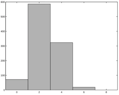
You can produce a histogram with the function^hist:

>> hist(randn(1000,1))

Here,^histis given 1000 points from the normal (0,1) random number generator. The result is shown in Figure 1.3.

You are now ready for more challenging computations. A random Fibonacci sequence^fxn^gis generated by choosingx1 andx2 and setting

xn+1=xnxn^;1; n2:

(27)

8 A Brief Tutorial

0 0.1 0.2 0.3 0.4 0.5 0.6 0.7 0.8 0.9 1

−0.8

−0.6

−0.4

−0.2 0 0.2 0.4 0.6 0.8

Figure 1.2. Basic 2D picture produced by ^plot.

−4 −3 −2 −1 0 1 2 3 4

0 50 100 150 200 250

Figure 1.3. Histogram produced by ^hist.

(28)

A Brief Tutorial 9

0 100 200 300 400 500 600 700 800 900 1000

10⁰ 10¹⁰ 10²⁰ 10³⁰ 10⁴⁰ 10⁵⁰ 10⁶⁰

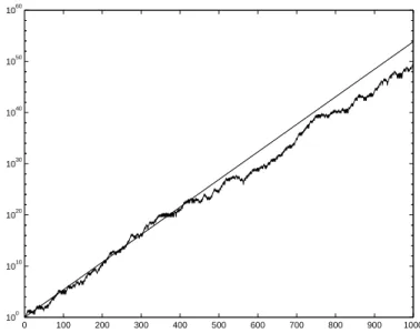
Figure 1.4. Growth of a random Fibonacci sequence.

Here, the indicates that + and ^; must have equal probability of being chosen.

Viswanath [82] analyzed this recurrence and showed that, with probability 1, for largenthe quantity^jxn^jincreases like a multiple ofcⁿ, wherec= 1:13198824:::(see also [17]). You can test Viswanath's result as follows:

>> clear

>> rand('state',100)

>> x = [1 2];

>> for n = 2:999, x(n+1) = x(n) + sign(rand-0.5)*x(n-1); end

>> semilogy(1:1000,abs(x))

>> c = 1.13198824;

>> hold on

>> semilogy(1:1000,c.^[1:1000])

>> hold off

Here,^clearremoves all variables from the workspace. The^forloop stores a random Fibonacci sequence in the array ^x; MATLAB automatically extends ^x each time a new element^x(n+1)is assigned. The^semilogy function then plots ⁿon the x-axis against^abs(x)on they-axis, with logarithmic scaling for they-axis. Typing^{hold on} tells MATLAB to superimpose the next picture on top of the current one. The second

semilogyplot produces a line of slope^c. The overall picture, shown in Figure 1.4, is consistent with Viswanath's theory.

The MATLAB commands to generate Figure 1.4 stretched over several lines. This is inconvenient for a number of reasons, not least because if a change is made to the experiment then it is necessary to reenter all the commands. To avoid this diculty you can employ a script M-le. Create an ASCII le named^rfib.midentical to List- ing 1.1 in your current directory. (Typing^editcalls up MATLAB's Editor/Debugger;

pwddisplays the current directory and^lsor^dirlists its contents.) Now type

>> rfib

(29)

10 A Brief Tutorial Listing 1.1. Script M-le^rfib.m.

%RFIB Random Fibonacci sequence.

rand('state',100) % Set random number state.

m = 1000; % Number of iterations.

x = [1 2]; % Initial conditions.

for n = 2:m-1 % Main loop.

x(n+1) = x(n) + sign(rand-0.5)*x(n-1);

end

semilogy(1:m,abs(x))

c = 1.13198824; % Viswanath's constant.

hold on

semilogy(1:m,c.^(1:m)) hold off

at the command line. This will reproduce the picture in Figure 1.4. Running^rfibin this way is essentially the same as typing the commands in the le at the command line, in sequence. Note that in Listing 1.1 blank lines and indentation are used to improve readability, and we have made the number of iterations a variable, ^m, so that it can be more easily changed. The script also contains helpful comments|

all text on a line after the ^%character is ignored by MATLAB. Having set up these commands in an M-le you are now free to experiment further. For example, changing

rand('state',100)torand('state',101)generates a dierent random Fibonacci sequence, and adding the linetitle('Random Fibonacci Sequence')at the end of the le will put a title on the graph.

Our next example involves the Collatz iteration, which, given a positive integer x1, has the formxk+1=f(xk), where

f(x) =

3x+ 1; ifxis odd, x=2; ifxis even.

In words: if x is odd, replace it by 3x+ 1, and if x is even, halve it. It has been conjectured that this iteration will always lead to a value of 1 (and hence thereafter cycle between 4, 2 and 1) whatever starting value x1 is chosen. There is ample computational evidence to support this conjecture, which is variously known as the Collatz problem, the 3x+ 1 problem, the Syracuse problem, Kakutani's problem, Hasse's algorithm, and Ulam's problem. However, a rigorous proof has so far eluded mathematicians. For further details, see [47] or type \Collatz problem" into your favorite Web search engine. You can investigate the conjecture by creating the script M-le^collatz.mshown in Listing 1.2. In this le a^whileloop and an^ifstatement are used to implement the iteration. The^inputcommand prompts you for a starting value. The appropriate response is to type an integer and then hit return or enter:

>> collatz

Enter an integer bigger than 2: 27

Here, the starting value ²⁷has been entered. The iteration terminates and the re- sulting picture is shown in Figure 1.5.

(30)

A Brief Tutorial 11

Listing 1.2. Script M-le^collatz.m.

%COLLATZ Collatz iteration.

n = input('Enter an integer bigger than 2: ');

narray = n;

count = 1;

while n ~= 1

if rem(n,2) == 1 % Remainder modulo 2.

n = 3*n+1;

else n = n/2;

end

count = count + 1;

narray(count) = n; % Store the current iterate.

end

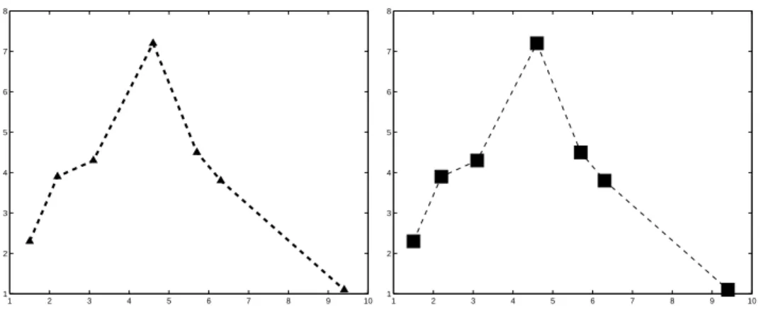
plot(narray,'*-') % Plot with * marker and solid line style.

title(['Collatz iteration starting at ' int2str(narray(1))],'FontSize',16)

0 20 40 60 80 100 120

0 1000 2000 3000 4000 5000 6000 7000 8000 9000 10000

Collatz iteration starting at 27

Figure 1.5. Plot produced by ^collatz.m.

(31)

12 A Brief Tutorial To investigate the Collatz problem further, the script^collbarin Listing 1.3 plots a bar graph of the number of iterations required to reach the value 1, for starting values 1;2;:::;29. The result is shown in Figure 1.6. For this picture, the function

gridadds grid lines that extend from the axis tick marks, and ^title, ^xlabeland

ylabeladd further information.

The well-known and much studied Mandelbrot set can be approximated graphi- cally in just a few lines of MATLAB. It is dened as the set of pointscin the complex plane for which the sequence generated by the mapz^7!z²+c, starting with z=c, remains bounded [65, Chap. 14]. The script^mandelin Listing 1.4 produces the plot of the Mandelbrot set shown in Figure 1.7. The script contains calls to^linspaceof the formlinspace(a,b,n), which generate an equally spaced vector ofⁿvalues between

aand^b. The^meshgridand^complexfunctions are used to construct a matrix^Cthat represents the rectangular region of interest in the complex plane. The^waitbarfunc- tion plots a bar showing the progress of the computation and illustrates MATLAB's Handle Graphics (the variable^his a \handle" to the bar). The plot itself is produced by^contourf, which plots a lled contour. The expressionabs(Z)<Z maxin the call to^contourfdetects points that have not exceeded the threshold^{Z max}and which are therefore assumed to lie in the Mandelbrot set. You can experiment with^mandelby changing the region that is plotted, via the^linspacecalls, the number of iterations

it max, and the threshold ^{Z max}.

Next we solve the ordinary dierential equation (ODE) system dtyd ¹⁽t) = 10(y2(t)^;y1(t));

dtyd ²⁽t) = 28y1(t)^;y2(t)^;y1(t)y3(t); dtyd ³⁽t) =y1(t)y2(t)^;8y3(t)=3:

This is an example from the Lorenz equations family; see [74]. We take initial condi- tionsy(0) = [0;1;0]^T and solve over 0t50. The M-le^lorenzdein Listing 1.5 is an example of a MATLAB function. Given^tand^y, this function returns the right- hand side of the ODE as the vector^yprime. This is the form required by MATLAB's ODE solving functions. The script ^lrunin Listing 1.6 uses the MATLAB function

ode45to solve the ODE numerically and then produces the (y1;y3) phase plane plot shown in Figure 1.8. You can see an animated plot of the solution by typing^lorenz, which calls one of MATLAB's demonstrations (type ^{help demos} for the complete list).

Now we give an example of a recursive function, that is, a function that calls itself. The Sierpinski gasket [64, Sec. 2.2] is based on the following process. Given a triangle with vertices Pa, Pb and Pc, we remove the triangle with vertices at the midpoints of the edges, (Pa +Pb)=2, (Pb +Pc)=2 and (Pc +Pa)=2. This removes the \middle quarter" of the triangle, as illustrated in Figure 1.9. Eectively, we have replaced the original triangle with three \subtriangles". We can now apply the middle quarter removal process to each of these subtriangles to generate nine subsubtriangles, and so on. The Sierpinski gasket is the set of all points that are never removed by repeated application of this process. The function ^gasketin Listing 1.7 implements the removal process. The input arguments ^Pa, ^Pband ^Pcdene the vertices of the triangle and^levelspecies how many times the process is to be applied. If ^levelis nonzero then ^gasketcalls itself three times with^levelreduced by 1, once for each

(32)

A Brief Tutorial 13 Listing 1.3. Script M-le^collbar.m.

%COLLBAR Collatz iteration bar graph.

N = 29; % Use starting values 1,2,...,N.

niter = zeros(N,1); % Preallocate array.

for i = 1:N count = 0;

n = i;

while n ~= 1

if rem(n,2) == 1 n = 3*n+1;

else n = n/2;

end

count = count + 1;

end

niter(i) = count;

end

bar(niter) % Bar graph.

grid % Add horizontal and vertical grid lines.

title('Collatz iteration counts','FontSize',16)

xlabel('Starting value','FontSize',16) % Label x axis.

ylabel('Number of iterations','FontSize',16) % Label y axis.

0 5 10 15 20 25 30

0 20 40 60 80 100 120

Collatz iteration counts

Starting value

Number of iterations

Figure 1.6. Plot produced by ^collbar.m.

(33)

14 A Brief Tutorial

Listing 1.4. Script M-le^mandel.m.

%MANDEL Mandelbrot set.

h = waitbar(0,'Computing...');

x = linspace(-2.1,0.6,301);

y = linspace(-1.1,1.1,301);

[X,Y] = meshgrid(x,y);

C = complex(X,Y);

Z_max = 1e6; it_max = 50;

Z = C;

for k = 1:it_max Z = Z.^2 + C;

waitbar(k/it_max) end

close(h)

contourf(x,y,abs(Z)<Z_max,1)

title('Mandelbrot Set','FontSize',16)

−2 −1.5 −1 −0.5 0 0.5

−1

−0.8

−0.6

−0.4

−0.2 0 0.2 0.4 0.6 0.8 1

Mandelbrot Set

Figure 1.7. Mandelbrot set approximation produced by^mandel.m.

(34)

A Brief Tutorial 15 Listing 1.5. Function M-le^lorenzde.m.

function yprime = lorenzde(t,y)

%LORENZDE Lorenz equations.

% YPRIME = LORENZDE(T,Y).

yprime = [10*(y(2)-y(1))

28*y(1)-y(2)-y(1)*y(3) y(1)*y(2)-8*y(3)/3];

Listing 1.6. Script M-le^lrun.m.

%LRUN ODE solving example: Lorenz.

tspan = [0 50]; % Solve for 0 <= t <= 50.

yzero = [0;1;0]; % Initial conditions.

[t,y] = ode45('lorenzde',tspan,yzero);

plot(y(:,1),y(:,3)) % (y_1,y_3) phase plane.

xlabel('y_1','FontSize',14)

ylabel('y_3 ','FontSize',14,'Rotation',0,'HorizontalAlignment','right') title('Lorenz equations','FontSize',16)

−200 −15 −10 −5 0 5 10 15 20

5 10 15 20 25 30 35 40 45 50

y1 y3

Lorenz equations

Figure 1.8. Phase plane plot from^ode45.

(35)

16 A Brief Tutorial Listing 1.7. Function M-le^gasket.m.

function gasket(Pa,Pb,Pc,level)

%GASKET Recursively generated Sierpinski gasket.

% GASKET(PA, PB, PC, LEVEL) generates an approximation to

% the Sierpinski gasket, where the 2-vectors PA, PB and PC

% define the triangle vertices.

% LEVEL is the level of recursion.

if level == 0

% Fill the triangle with vertices Pa, Pb, Pc.

fill([Pa(1),Pb(1),Pc(1)],[Pa(2),Pb(2),Pc(2)],[0.5 0.5 0.5]);

hold on else

% Recursive calls for the three subtriangles.

gasket(Pa,(Pa+Pb)/2,(Pa+Pc)/2,level-1) gasket(Pb,(Pb+Pa)/2,(Pb+Pc)/2,level-1) gasket(Pc,(Pc+Pa)/2,(Pc+Pb)/2,level-1) end

of the three subtriangles. When ^levelnally reaches zero, the appropriate triangle is drawn. The following code generates Figure 1.10.

>> level = 5;

>> Pa = [0;0];

>> Pb = [1;0];

>> Pc = [0.5;sqrt(3)/2];

>> gasket(Pa,Pb,Pc,level)

>> hold off

>> title(['Gasket level = ' num2str(level)],'FontSize',16)

>> axis('equal','off')

(Figure 1.9 was generated in the same way with ^{level = 1}.) In the last line, the call to ^axismakes the units of the x- and y-axes equal and turns o the axes and their labels. You should experiment with dierent initial vertices^Pa,^Pband^Pc, and dierent levels of recursion, but keep in mind that setting^levelbigger than 8 may overstretch either your patience or your computer's resources.

The Sierpinski gasket can also be generated by playing Barnsley's \chaos game"

[64, Sec. 1.3]. We choose one of the vertices of a triangle as a starting point. Then we pick one of the three vertices at random, take the midpoint of the line joining this vertex with the starting point and plot this new point. Then we take the midpoint of this point and a randomly chosen vertex as the next point, which is plotted, and the process continues. The script ^barnsley in Listing 1.8 implements the game.

Figure 1.11 shows the result of choosing 1000 iterations:

>> barnsley

Enter number of points (try 1000) 1000

Try experimenting with the number of points,ⁿ, the type and size of marker in the

plotcommand, and the location of the starting point.

(36)

A Brief Tutorial 17

Gasket level = 1

Figure 1.9. Removal process for the Sierpinski gasket.

Gasket level = 5

Figure 1.10. Level 5 Sierpinski gasket approximation from ^gasket.m.

(37)

18 A Brief Tutorial

Listing 1.8. Script M-le^barnsley.m.

%BARNSLEY Barnsley's game to compute Sierpinski gasket.

rand('state',1) % Set random number state.

V = [0, 1, 0.5; 0, 0, sqrt(3)/2]; % Columns give triangle vertices.

point = V(:,1); % Start at a vertex.

n = input('Enter number of points (try 1000) ');

for k = 1:n

node = ceil(3*rand); % node is 1, 2 or 3 with equal prob.

point = (V(:,node) + point)/2;

plot(point(1),point(2),'.','MarkerSize',15) hold on

end

axis('equal','off') hold off

Figure 1.11. Sierpinski gasket approximation from^barnsley.m.

(38)

A Brief Tutorial 19

Listing 1.9. Script M-le^sweep.m.

%SWEEP Generates a volume-swept 3D object.

N = 10; % Number of increments - try increasing.

z = linspace(-5,5,N)';

radius = sqrt(1+z.^2); % Try changing SQRT to some other function.

theta = 2*pi*linspace(0,1,N);

X = radius*cos(theta);

Y = radius*sin(theta);

Z = z(:,ones(1,N));

surf(X,Y,Z) axis equal

−4

−2 0

2 4

−5 0

5

−5 0 5

Figure 1.12. 3D picture produced by ^sweep.m.

(39)

20 A Brief Tutorial We nish with the script^sweepin Listing 1.9, which generates a volume-swept three-dimensional (3D) object; see Figure 1.12. Here, the commandsurf(X,Y,Z)cre- ates a 3D surface where the height^Z(i,j)is specied at the point(X(i,j),Y(i,j))

in thex-y plane. The script is not written in the most obvious fashion, which would use two nested ^forloops. Instead it is vectorized. To understand how it works you will need to be familiar with Chapter 5 and Section 21.4. You can experiment with the script by changing the parameter^Nand the function that determines the variable

radius: try replacing^sqrtby other functions, such as^log,^sinor^abs.

If you are one of those experts who wants to see something from MATLAB right now and would rather read the instructions later, this page is for you.

| 386-MATLAB User's Guide (1989) Do not be too timid and squeamish about your actions.

All life is an experiment.

The more experiments you make the better.

| RALPH WALDO EMERSON

(40)

Chapter 2 Basics

2.1. Interaction and Script Files

MATLAB is an interactive system. You type commands at the prompt (^>>) in the Command Window and computations are performed when you press the enter or return key. At its simplest level, MATLAB can be used like a pocket calculator:

>> (1+sqrt(5))/2 ans =

1.6180

>> 2^(-53) ans =

1.1102e-016

The rst example computes (1 +^p5)=2 and the second 2^;⁵³. Note that the second result is displayed in exponential notation: it represents 1:110210^;¹⁶. The variable

ansis created (or overwritten, if it already exists) when an expression is not assigned to a variable. It can be referenced later, just like any other variable. Unlike in most programming languages, variables are not declared prior to use but are created by MATLAB when they are assigned:

>> x = sin(22) x =

-0.0089

Here we have assigned to ^x the sine of 22 radians. The printing of output can be suppressed by appending a semicolon. The next example assigns a value to^ywithout displaying the result:

>> y = 2*x + exp(-3)/(1+cos(.1));

Commas or semicolons are used to separate statements that appear on the same line:

>> x = 2, y = cos(.3), z = 3*x*y x =

2 y =

0.9553 z =

5.7320

>> x = 5; y = cos(.5); z = x*y^2

21

(41)

22 Basics

z =

3.8508

Note again that the semicolon causes output to be suppressed.

MATLAB is case sensitive. This means, for example, that ^x and ^X are distinct variables.

To perform a sequence of related commands, you can write them into a script M- le, which is a text le with a^.mlename extension. For example, suppose you wish to process a set of exam marks using the MATLAB functions ^sort, ^mean, ^median and ^std, which, respectively, sort into increasing order and compute the arithmetic mean, the median and the standard deviation. You can create a le, say^marks.m, of the form

%MARKS

exmark = [12 0 5 28 87 3 56];

exsort = sort(exmark) exmean = mean(exmark) exmed = median(exmark) exstd = std(exmark)

The^%denotes a comment line. Typing

>> marks

at the command line then produces the output

exsort =

0 3 5 12 28 56 87

exmean = 27.2857 exmed =

12 exstd =

32.8010

Note that calling ^marksis entirely equivalent to typing each of the individual commands in sequence at the command line. More details on creating and using script les can be found in Chapter 7.

Throughout this book, unless otherwise indicated, the prompt^>> signals an example that has been typed at the command line and it is immediately followed by MATLAB's output (if any). A sequence of MATLAB commands without the prompt should be interpreted as forming a script le (or part of one).

To quit MATLAB type^exitor^quit.

2.2. More Fundamentals

MATLAB has many useful functions in addition to the usual ones found on a pocket calculator. For example, you can set up a random matrix of order 3 by typing

>> A = rand(3) A =

0.9501 0.4860 0.4565 0.2311 0.8913 0.0185 0.6068 0.7621 0.8214

(42)

2.2 More Fundamentals 23 Here each entry of Âis chosen independently from the uniform distribution on the interval [0;1]. Theînvcommand invertsÂ:

>> inv(A) ans =

1.6740 -0.1196 -0.9276 -0.4165 1.1738 0.2050 -0.8504 -1.0006 1.7125

The inverse has the property that its product with the matrix is the identity matrix.

We can check this property for our example by typing

>> ans*A ans =

1.0000 0.0000 -0.0000 0.0000 1.0000 0.0000 0.0000 -0.0000 1.0000

The product has 1s on the diagonal, as expected. The o-diagonal elements, displayed as plus or minus^0.0000, are, in fact, not exactly zero. MATLAB stores numbers and computes to a relative precision of about 16 decimal digits. By default it displays numbers in a 5-digit xed point format. While concise, this is not always the most useful format. The^formatcommand can be used to set a 5-digit oating point format (also known as scientic or exponential notation):

>> format short e

>> ans ans =

1.0000e+000 7.4485e-017 -8.9772e-017 1.3986e-017 1.0000e+000 9.7172e-018 7.4159e-017 -7.9580e-017 1.0000e+000

Now we see that the o-diagonal elements of the product are nonzero but tiny|

the result of rounding errors. The default format can be reinstated by typing^format

short, or simply^format. The^formatcommand has many options, which can be seen by typing help format. See Table 2.1 for some examples. All the MATLAB output shown in this book was generated with format compactin eect, which suppresses blank lines.

Generally,^{help foo}displays information on the command or function named^foo. For example:

>> help sqrt

SQRT Square root.

SQRT(X) is the square root of the elements of X. Complex results are produced if X is not positive.