Extracting Risk-Neutral Probability Distributions from Option Prices Using Trading Volume as a Filter

IHS Economics Series Working Paper 104

September 2001

Extracting Risk-Neutral Probability Distributions from Option Prices Using Trading Volume as a Filter

Dominique Y. Dupont

Impressum Author(s):

Dominique Y. Dupont Title:

Extracting Risk-Neutral Probability Distributions from Option Prices Using Trading Volume as a Filter

ISSN: Unspecified

2001 Institut für Höhere Studien - Institute for Advanced Studies (IHS) Josefstädter Straße 39, A-1080 Wien

E-Mail: o ce@ihs.ac.atffi Web: ww w .ihs.ac. a t

All IHS Working Papers are available online: http://irihs. ihs. ac.at/view/ihs_series/

This paper is available for download without charge at:

https://irihs.ihs.ac.at/id/eprint/1367/

Extracting Risk-neutral Probability Distributions from Option Prices Using Trading Volume as a Filter

Dominique Y. Dupont

104

Reihe Ökonomie

Economics Series

104 Reihe Ökonomie Economics Series

Extracting Risk-neutral Probability Distributions from Option Prices Using Trading Volume as a Filter

Dominique Y. Dupont

September 2001

Contact:

Dominique Y. Dupont EURANDOM – TUE P.O. Box 513

NL-5600 MB Eindhoven The Netherlands (: +31 / 40 / 247 8123 fax: +31 / 40 / 247 8190 email: dupont@eurandom.tue.nl

Founded in 1963 by two prominent Austrians living in exile – the sociologist Paul F. Lazarsfeld and the economist Oskar Morgenstern – with the financial support from the Ford Foundation, the Austrian Federal Ministry of Education and the City of Vienna, the Institute for Advanced Studies (IHS) is the first institution for postgraduate education and research in economics and the social sciences in Austria. The Economics Series presents research done at the Department of Economics and Finance and aims to share “work in progress” in a timely way before formal publication. As usual, authors bear full responsibility for the content of their contributions.

Das Institut für Höhere Studien (IHS) wurde im Jahr 1963 von zwei prominenten Exilösterreichern – dem Soziologen Paul F. Lazarsfeld und dem Ökonomen Oskar Morgenstern – mit Hilfe der Ford- Stiftung, des Österreichischen Bundesministeriums für Unterricht und der Stadt Wien gegründet und ist somit die erste nachuniversitäre Lehr- und Forschungsstätte für die Sozial- und Wirtschafts- wissenschaften in Österreich. Die Reihe Ökonomie bietet Einblick in die Forschungsarbeit der Abteilung für Ökonomie und Finanzwirtschaft und verfolgt das Ziel, abteilungsinterne

Abstract

This paper introduces a new technique to infer the risk-neutral probability distribution of an asset from the prices of options on this asset. The technique is based on using the trading volume of each option as a proxy of the informativeness of the option. Not requiring the implied probability distribution to recover exactly the market prices of the options allows us to weight each option by a function of its trading volume. As a result, we obtain implied probability distributions that are both smoother and should be more reflective of fundamentals.

Keywords

Implied risk-neutral probability distribution, implied-tree method

JEL Classifications

G13, G14

Comments

Contents

1 Current Methods to Compute Risk-Neutral Probability

Distributions 2

1.1 Definitions ... 2 1.2 Retrieving risk-neutral distributions when there are as many states of the world as

traded assets ... 3 1.3 Retrieving risk-neutral distributions when there are more states of the world than

traded assets ... 5

2 A New Non-Parametric Method to Compute Risk-Neutral

Probability Distributions from the Prices of Traded Assets 7

3 Early Exercise 10

4 Application 12

4.1 Data ... 12 4.2 Results ... 14

5 Conclusion 18

Appendix 20

A Retrieving risk-neutral distributions when there are as many marketable assets as states of the world ... 20 B More states than marketable assets ... 21

References 22

Tables and Figures 24

Trading activity in derivatives products, whether on organized exchanges or on over-the-counter (OTC) markets has increased dramatically in the past fteen years and derivatives have become a mainstay of nancial mar- kets.

Standard, plain-vanilla contracts are very liquid and trading data on exchange-traded products are publicly available. Derivatives prices can be used to extract information on the probability distributions of the underly- ing assets because the payos of derivatives contracts depend on the future values of the underlying assets. This information is of use not only to deriva- tives traders but also to a wider public, including holders of the underlying securities and policy makers.

Dierent instruments are used to infer dierent characteristics of the dis- tribution of the underlying asset. Quotes on futures contracts give some in- formation on the market's expectations of the underlying asset price; option prices provide a measure of the dispersion of the asset price around its mean, the implied volatility, which can be used to gauge the degree of uncertainty prevalent in the markets.

If the Black-Scholes theory were true, the implied volatility would be constant across strikes and would suce to describe the whole distribution of the underlying asset. In practice, implied volatilities are not constant across strikes. Fortunately, combinations of options can yield information about the distribution of the underlying asset without the need for a priori assumptions. Bates (1991) devises a technique using option prices to estimate the skewness of the distribution of the underlying asset. If quotes on European options were available for a continuum of strike prices, one could use the method of Breeden and Litzenberger (1978) to retrieve the entire probability density function (thereafter, "pdf") of a given asset.

In this case, the implied probability distribution would subsume the Bates skewness measure.

In practice, strike prices, or strikes for short, are available only at discrete intervals. If one assumes that all possible future values of the underlying as- set coincide with the available strikes, the probability distribution of the asset could be uniquely recovered from the available option prices. Alterna- tively, the researcher could assume that the asset can take values other than the available strikes and strive to obtain a distribution consistent with the observed option prices. Because multiple distributions are consistent with the option prices in that case, some additional selection criteria is needed.

The researcher may conjecture a functional form for the implied pdf and choose the parameters to replicate as well as possible the market prices of the options, or, alternatively, use non-parametric methods. Whatever the techniques used to construct them, implied probability distributions have become popular analysis tools. Some economists, like Campa et al. (1997), Melick and Thomas (1997, 1998), and Soderling and Svensson (1997) use

1

The notional amount of interest rate, currency, and equity futures and options has increased almost twentyfold between 1986 and 1997 (IMF, 1998). More recent data point to a 30-percent increase in the notional amount of OTC derivatives between June 1998 and June 2000 (BIS, 2000)

2

The implied volatility of an option at a given strike is the volatility at which the price

of the option assigned by the Black-Scholes (1973) formula coincides with the market price

of the option.

option-based probability distributions to gauge the immediate market im- pact of some particular event (Table 1). Others, like Rubinstein (1994), Jackwerth and Rubinstein (1996), and Stutzer (1996) use option prices to compare implied probability distributions across longer time horizons, for ex- ample several years before and after the crash of 1987, or to build time-series of some characteristics of the distribution, like skewness and kurtosis.

Current non-parametric approaches typically try to force the probability distribution to perfectly replicate the market prices of the options. Instead, we choose to only impose a non-replication cost in the objective function and trade o increased smoothness of the implied pdf against lower goodness of t with the market prices of the options. The advantage of this method is that one can weight each option price by a proxy of its informativeness. We select trading volume as such a proxy because there are strong economic arguments to think that asset prices contain more information when these assets are more actively traded.

1 Current Methods to Compute Risk-Neutral Prob- ability Distributions

The following section introduces a simple two-period framework to review the concept of risk-neutral distribution and presents several methods designed to retrieve such probability distributions from option prices.

1.1 Denitions

Risk in the economy is generated by the random payo of a single asset, S , which can take n possible values in the second period and is referred to as the

"underlying asset." Agents can trade several assets in the rst period that all pay out in the second period: m European call options on the underlying asset, a forward contract on the same asset, and a riskless bond. Each of the realizations of S denes a "state of the world." There is no transaction costs or restrictions to trade, and the market is free of arbitrage. We assume without loss of generality that the options are calls; prices of European puts can always be translated into equivalent call prices using the put-call parity.

The following theorem presents a well-known result in nancial economics.

Theorem 1

If market prices are arbitrage-free, there exists a probability distribution, P, such that, if ( x ) is the price of a claim paying out x in the last period,

( x ) = E ^P [ e

^r x ] (1) where is the time between the two periods, r is the (xed) interest rate, and E ^P [ ] denotes the expectation against P . This probability distribution is called "risk-neutral."

Proof:

Call x i the realization of asset x when S = S i , z i the random variable

that pays $1 when S = S i and $0 otherwise ( z i is the "state-contingent

claim" for the i ^th state), and let p i = e ^r ( z i ). Then, because the function is linear and x =

ⁿ _i

x i z i ,

( x ) =

ⁿ

i

e

^r x i p i : (2)

The p i 's are positive because is assumed to admit no arbitrage opportu- nities and they sum up to 1 because the riskless bond, which pays $1 in every state and is worth by denition e

^r can be replicated by holding all contingent claims. Hence, the p i 's dene a probability distribution, P , and ( x ) = E ^P [ e

^r x ].

In the following, we review several techniques to construct (risk-neutral) probability distributions consistent with the prices of selected assets.

Notations: C ( K j ) is the price of a call option struck at K j , j = 1 ;::: ;m , and F is the forward price of the underlying asset.

Corollary: A series of non-negative scalars p i , i = 1 ;:::;n , denes a risk- neutral probability distribution consistent with the prices of the traded assets if and only if

8

<

: P

n

i

p i e

^r max(0 ;S i

K j ) = C ( K j ) ;

P

n i

p i S i = F;

P

n i

p i = 1 : ⁽³⁾

Eq. (3) denes a system of m + 2 equations in n unknowns (the p i 's) and is equivalent to the matrix equality

M : P = Q (4)

where P = ( p i ) _ni

, Q gathers the m + 2 terms in the right-hand side of the equation, and M is a m + 2

n matrix obtained from the left-hand side of the equation.

The "risk-neutral" distribution combines characteristics of the "real- world" probability distribution and the market participants' appetite for risk. Nonetheless, quotes on derivative instruments taken at two moments in time can give information on the evolution of the real-world probability distribution of the underlying asset if attitudes toward risk are assumed to remain constant in the interval.

If there are as many derivatives assets as states of the world, the risk- neutral probability distribution is unique and can be inferred from the option prices in an intuitive manner. If there are more states of the world than derivatives, the researcher can use parametric or non-parametric methods to pin down one risk-neutral probability distribution.

1.2 Retrieving risk-neutral distributions when there are as many states of the world as traded assets

Setting the number of states of the world equal to the number of assets

( n = m + 2) and ignoring the positivity constraint on the risk-neutral prob-

abilities, one can easily recover the unique risk-neutral probability distribu- tion. Assume that the spacing between two strike prices is constant and equal to . Dene the possible realizations of S as follows

8

<

:

S

= K

;

S i = K i

for i = 2 ;:::;m + 1 ;

S m

= K m + : ⁽⁵⁾

With n = m + 2, the system dened in Eq. (3) admits a unique and simple solution. The implied probabilities of states in the heart of the distribution match those obtained using the "buttery spread" strategy of Breeden and Litzenberger (1978). More precisely, if K i is not the lowest or the highest strike, a trader can replicate the claim paying out $1 when S = K i and nothing otherwise by taking a long position in 1 = calls struck at K i

and K i

, and a short position in 2 = calls struck at K i (see Appendix). The procedure is illustrated graphically in Figure 1. The risk-neutral probability of the state " S = K i " is

P ( S = K i ) = p i

= e ^r ( C ( K i

)

2 C ( K i ) + C ( K i

)) = : (6) The probability in the tails of the distribution dened in Eq. (4) can be recovered using a simple trading strategy and the fact that probabilities sum up to 1.

P ( S

K m ) = p m

+ p m

= e ^r ( C ( K m

)

C ( K m )) = ; P ( S

K

) = p

+ p

= 1

^m _i

p i : ⁽⁷⁾ Taking into account the underlying asset and the riskless bond enables us to extend the range of the distribution beyond the lowest and the highest strikes.

The density function at S = K is f ( K ) = P ( S = K ) = and hence f ( K ) = e ^r

C ( K

)

2 C ( K ) + C ( K + )

=

: (8) f ( K ) is the nite-dierence approximation of e ^{r @}

_@K ^C

^K

. More generally, as shown in Breeden and Litzenberger (1978), if S takes a continuum of possible values and each of those is the strike price of a call option, the risk-neutral probability density function away from the boundaries of the distribution is

f ( K ) = e ^r @

C ( K )

@K

: (9)

No positivity constraint need to be imposed on the probability density func- tions dened in Eqs. (8) and (9) because the price of an option is a con- vex function of the strike.

However, option prices observed in the market are not always convex in their strikes because of transaction costs or non- synchronous trading.

3

This is the case when the underlying price process is a one-dimensional diusion and

in some stochastic-volatility models (Bergman et al., 1996).

In the present framework, one can replicate the payos of the contingent claims, and hence of any asset, by forming portfolios of the options: the market is "complete" and a unique risk-neutral distribution is inferred from option prices. In practice, m is given and the researcher decides n , that is, makes markets complete by constraining the possible realizations of the underlying asset. The fewer the strike prices, the more constraining this approach is.

Alternatively, we can consider that there are more states than traded assets and construct a risk-neutral probability distribution consistent with the prices of the traded options.

1.3 Retrieving risk-neutral distributions when there are more states of the world than traded assets

Creating more states than traded assets enables one to rene the grid of the support of the probability distribution and to extend the tails of the distribution farther away from the lowest and highest strikes. With more states than assets, markets are incomplete and multiple risk-neutral distri- butions can t the option prices. In other words, when n > m +2, there are more unknowns than equations in the linear system dened by Eq. (3) and the system admits multiple solutions. One needs some additional criteria to pin down a unique probability distribution. One solution is to impose a functional form for the probability distribution and to estimate its param- eters using the option data. Alternatively, one can choose non-parametric methods, which can deliver implied distributions that perfectly match the option prices observed in the market. Even though not all non-parametric methods aim at perfectly replicating the market prices of derivatives, their extra exibility allows a closer t with market prices.

Non-parametric methods

One such method consists in minimizing the Euclidean distance between the distribution that ts the option prices, P , and an initial distribution, P

. This is based on the "implied-tree method" of Rubinstein (1994).

The implied-trees of Rubinstein (1994) and Jackwerth and Rubinstein (1996) only require the option prices obtained from the risk-neutral pdf to be between the bid and ask prices observed in the market. When only closing or settlement prices are available, the implied-tree procedure typically constrains the pdf to exactly recover the market prices of the options (Campa et al., 1998).

Mathematically, the objective is to min _p

i

n

X

i

( p i

p

_i )

(10)

subject to the constraints of Eq. (3) and

p i

0 for i = 1 ;:::;n: (11)

4

The original article by Rubinstein used binomial trees. However, the method is called

"implied trees" even if no tree is used.

Eq. (3) imposes m + 2 conditions on the n risk-neutral probabilities p i 's.

Consequently, the n -dimensional vector P can be expressed as a linear func- tion of n

m

2 of its components and of the prices of the marketed assets.

Using this relation and the rst-order conditions implied in Eq. (10) while ignoring the non-negativity constraints on the p i 's, one can easily solve for P as a linear function of the price of the marketed assets (see Appendix).

The quadratic distance function in Eq. (10) can be replaced by the

\entropy" criterion function of Stutzer (1996), and Buchen and Kelly (1997):

min _p

i

n

X

i

p i log( p i =p

_i ) : (12)

Eq. (12) guarantees the positivity of the risk-neutral probabilities. Using Eq. (12) or using Eq. (10) with p i

0 result in a non-linear optimization problem requiring the use of numerical solution techniques. For the sake of computational simplicity, we use the quadratic distance function without imposing positivity of the risk-neutral probabilities.

Parametric methods

An alternative to these non-parametric methods is to impose a exible but parametric form on the probability distribution and determine its parame- ters by maximizing the t of the option prices implied by the probability distribution to the prices observed in the market. (The objective function to minimize typically is the sum of the square dierences between the option prices implied by the distribution and those observed in the market.) The additional structure provided by parametric methods may reduce the risk of overtting the data but option prices based on the risk-neutral probability distribution fail to coincide exactly with those observed in the market. How- ever, the researcher can improve the t by allowing more exibility in the parametric function (at the cost of an increase in the numerical complexity of the optimization problem).

Melick and Thomas (1997) assume that the price of the underlying asset follows a mixture of N lognormals, that is, that the risk-neutral density function g is dened by

g ( t ) =

^N

i

i g i ( t ) ; (13)

where

g i ( t ) = 1

2 i t ^exp

"

1 2

log( t )

i ) i

2

#

; (14)

and

N

i

i = 1 : (15)

5

When such constraints are imposed, perfect replication of the option prices is not

guaranteed.

The more lognormal distributions are included, the better the t with the observed option prices but the more dicult the estimation procedure may be. Numerical diculties seem to limit the choice of N to 2 to 3 in practice.

Anecdotally, a change-of-regime model where the asset price at maturity fol- lows distribution g i with probability i yields the density function of Eq. (13) but reference to this model is not necessary and the mixture-of-distribution method can be seen in its own right as a way to obtain a parametric proba- bility distribution that closely matches options prices.

Soderling and Svensson (1997) point out that the mix-of-distribution approach sometimes generates implied pdfs with sharp spikes, and that the loss function (the minimization of which yields estimates of the parameters) is often very at. This could cause the implausibly large changes in the shape of the pdfs between consecutive days observed by Clews et al. (2000).

Jackwerth (1999) conrms that the mixture-of-distribution method tends to overt the data when many distributions are used in the mix. Even if the overall shape of the distribution is roughly stable across short periods of time, individual distributions in the mix can change drastically, which invalidates the use of the method in estimating a change-of-regime model.

2 A New Non-Parametric Method to Compute Risk- Neutral Probability Distributions from the Prices of Traded Assets

The method introduced below is both an extension and a simplication of implied trees. The implied-tree method above forces the risk-neutral proba- bility distribution to exactly replicate the option prices. However, one may not wish to match all quoted options prices exactly if some poorly reect eco- nomic fundamentals. This paper innovates by substituting a penalty for not matching the option prices instead of the obligation of recovering them ex- actly. Not tting the option prices perfectly allows us to weight each option price by its trading volume, which we use as a proxy for the informativeness of the option's price. In other words, highly traded options are assumed to contain more information than low-volume options.

Trading volume is typically very unequally distributed across strike prices.

Clews et al. (2000) note that at- and near-the-money options account for most of trading volume in options on Financial Times Share 100 Index (FTSE 100) and on short-term sterling interest-rate futures. Recent data on options on Eurodollar, Standard and Poors 500 Index (S&P 500) futures re- veals the same pattern. Exchanges typically publish daily settlement prices for options that have not been traded on the day. Such quotes are model based and should not be used to construct implied probability distributions.

It is also doubtful whether prices of options with very low trading volume are meaningful.

Economic motivations for using trading volume as a lter

There are several reasons to weight each option by its trading volume. The

equilibrium price of an asset averages the dierent values assigned to the

asset by the participating traders. Intuitively, if buying and selling orders contain some noise, the latter should have a lesser impact on highly traded options because the idiosyncratic components of the order ow are averaged across a larger pool of traders. This should lead us to give more weight to high-volume options, following the example of generalized least-squares re- gressions, which deal with variables that are means of other random variables by weighting each observation by the size of the sample it averages.

Another reason to use trading volume to discriminate among the dier- ent options is that quotes on high-volume options are more likely to corre- spond to simultaneous transactions. Transaction volume typically displays a U-shape pattern across the trading day (Jain and Joh, 1988). Since set- tlement prices of exchange-traded derivatives most often coincide with their prices at the close, quotes on high-volume options are likely to correspond to transactions occurring during the peak-volume time at the end of the trading session. Put another way, options with low cumulative trading vol- ume on the day are more likely to have stopped trading during the relative low-activity period in the middle of the day. Scaling down the importance of low-volume options adapts end-of-day data to a technique, risk-neutral probability inference, that assumes that all option prices are determined simultaneously.

One justication for using trading volume to discriminate among options on the same underlying asset is grounded in economic theory: Models de- veloped by Human (1992) and Blume, Easley, and O'Hara (1994) suggest that trading volume is higher when the agents' information about the true value of the traded asset is more precise. Although the lack of reliable in- dicator of the precision of traders' information hinders the testing of this proposition, other predictions of these models are clearly borne out by the data. For example, there is strong empirical support for the positive cor- relation between trading volume and the absolute dierence of the price of an asset predicted by both these models, as documented by Karpo (1987), and Gallant, Rossi, and Tauchen (1992). Using a general-equilibrium econ- omy where dierently-informed agents exchange productive capital, Hu- man (1992) obtains a strong relationship between the transaction volume of capital and a measure of its informativeness about the future state of the economy. Blume, Easley, and O'Hara (1994) investigate the informational role of trading volume in a noisy rational-expectations exchange economy where the precision of the private signals observed by the traders is random.

The equilibrium trading volume is an increasing function of the precision of the private signals and conveys information not revealed by the equilibrium price. Dupont (1997) uses a noisy rational-expectations framework where the precision of the informed traders' signals is deterministic but the sig- nals' correlation structure is richer than that in Blume, Easley, and O'Hara (1994). The mean trading volume and the informativeness of the equilib- rium market price, measured by its correlation with the true value of the traded asset, display very similar patterns to changes in the precision of the informed traders' private signals or in the correlation between their signals.

Both the mean trading volume and the informativeness of the market price

are increasing in the precision of the private signals and decreasing in the

correlation between those signals. The latter pattern conrms the conclu- sion of Shalen (1993) whose model generates a positive relation between the dispersion of the traders' beliefs.

A simple method to use trading volume as a lter

The method presented in this paper weights every option by a function of its trading volume. To simplify, we neglect the early exercise clause of the (American) options used and do not impose non-negativity constraints on the implied probabilities. As shown in the next section, the early-exercise feature does not seem to have much impact on the prices of options that are not very far in the money. Ignoring positivity constraints allows us to solve the optimization problem in closed form, using only linear algebra, because the loss function is quadratic and the constraints linear in the implied prob- abilities, so that the implied probabilities are linear in the option prices. In contrast, Jackwerth and Rubinstein (1997) impose positivity constraints on the implied probabilities and use an advanced algorithm (Broyden-Fletcher- Goldfarb-Shanno) to compute them. Even those who prefer to use non-linear optimization techniques to guarantee non-negative probabilities may be in- terested in having a simpler, faster procedure ready, especially if they have to recover implied probabilities daily or on demand.

The option prices can be weighted by their trading volume or a function of their trading volume. We impose that options with zero volume be given zero weight. We experiment with two specications. Let _si be the weight allocated to the option struck at K i by specication s and V ( i ) be the trading volume of this option.

_i = V ( i ) =

^m _k

V ( k ) ;

_i = log(1 + V ( i )) =

^m _k

log(1 + V ( k )) : ⁽¹⁶⁾ The second specication gives high-volume options less predominance than the rst. One could also exclude options whose trading volume is below a threshold.

Moreover, we fully use the exibility oered by the non-parametric char- acter of the implied-tree method. For example, we choose dierent distribu- tions to build the initial p

_i 's probabilities. In the heart of the distribution, that is, for prices above the minimum strike and below the maximum strike, the p

_i 's are generated by a lognormal distribution with a volatility that min- imizes the average square deviation between the asset prices implied by the distribution and the asset prices observed in the market. In contrast, the p

_i 's in the tails of the distribution, are generated by a lognormal distribu- tion with a higher volatility. The increase in the volatility of the lognormal distribution which serves as a reference in the estimation of the implied risk- neutral distribution matches the observation that implied volatilities tend to be higher for strikes prices further away from the center of the distribution.

We also impose a quadratic smoothness criteria on the implied probabili-

ties. Using this smoothness criteria, we can dispense with imposing that the

implied probabilities be close to initial probabilities in the heart of the distri-

bution for the options on Eurodollar futures (but not for those on S&P 500

futures). However, it is still advisable to impose closeness to a well-behaved

distribution in the tails. A major advantage of implied-tree methods over parametric approaches is that the user can easily tailor the method to his own needs.

The new objective function is ( P ) =

_i

_I ( p i

p

_i )

+

^m _j

j

n

i

p i e

^r max(0 ;S i

K j )

C ( K j )

+

ⁿ _i

p i S i

F +

ⁿ _i

p i

1

+ (1

)

ⁿ _i

( p i

2 p i + p i

)

; ⁽¹⁷⁾ where the i 's are the weights on the constraints, I indexes the p i 's for which a cost of deviating from the initial probabilities p

_i 's is imposed, and the i 's are the weights on the prices of the options observed in the market.

To express Eq. (17) in matrix form, write S

= Diag( I [ i

I ]) ;

= Diag(

;:::; m ; 1 ; 1) ; ⁽¹⁸⁾ and let R the matrix so that P

RP =

ⁿ _i

( p i

2 p i + p i

)

. The objective function becomes

( P ) =

( P

P

)

S

( P

P

) +

( M P

Q )

( MP

Q ) + (1

) P

RP;

(19) where the matrices M and Q follow from Eq. (4). The solution is, assuming invertibility of the relevant matrix,

P =

S

+

M

M + (1

) R

(

S

P

+

M

Q ) : (20)

3 Early exercise

In this section, we review the impact of the early-exercise feature on the prices of American-style options and the special character of options that are very far in the money.

Many options traded on nancial exchanges can be exercised at any time before expiry. Melick and Thomas (1997) take this early-exercise feature into account by letting the model price of the option be a weighted average of the upper and lower bounds on American options and by making the weight a parameter of the objective function. As an alternative, Pirkner, Weigend, and Zimmermann (1999) combine the mixture-of-distribution method and implied binomial trees to capture the path-dependency generated by the early-exercise clause. Clews et al. (2000) use the mixture-of-distribution technique but adjust for the early exercise premium using the method de- veloped by Barone-Adesi and Whaley (1987).

6

The underlying asset is now assumed to be a futures contract, so that the prices of

American and European calls dier. In contrast, these prices coincide when the underlying

asset is a stock that pays no dividend.

However, recent research suggests that the early-exercise feature of traded options could be ignored. Soderling and Svensson (1997) compare the im- plied pdfs obtained using the method of Melick and Thomas (1997) to those obtained using the mixture-of-distribution technique while treating Ameri- can options as though they were European options. They report that the two pdfs are indistinguishable to the eye and that "the correction for American- style is not important, at least not compared to pricing errors (which possibly reect some other type of misspecication)" [p. 405].

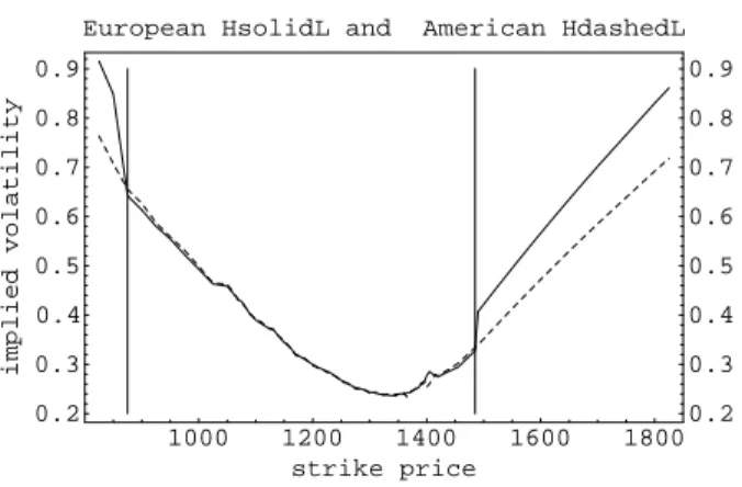
To gauge the impact of the early exercise feature on option prices, we computed the implied volatilities of options on S&P 500 index futures traded on the Chicago Mercantile Exchange (CME) neglecting and taking account of the Americanness of these options (Figure 2). Except for options very far in-the-money, the implied volatilities are identical across the two methods.

We show below why far-in-the-money options should be treated dierently than other options (or excluded entirely).

Since American-style options can be exercised at any time, no-arbitrage lower bounds on their values are immediate. If F t is the price of the under- lying asset (a futures contract), C t ( F t ;K ) the price of a call option struck at K , and P t ( F t ;K ) the price of a put option struck at K , then

C t ( F t ;K )

F t

K;

P t ( F t ;K )

K

F t : ⁽²¹⁾ The right-hand side of Eq. (21) represent the payment obtained from exercis- ing the option when it is cash-settled or the net prot of exercising the option and taking a counterbalancing trade in the underlying asset otherwise. Little information about the future realizations of the underlying asset value can be inferred from options whose prices coincide with their lower bounds. For example, assume the underlying asset follows a geometric Brownian motion, as in Black-Scholes. If the theoretical price of an American call coincides with the market price of the option for a volatility when the market price hits its lower bound, any volatility lower than will also be consistent with the observed option price.

This relates to the trade-o faced by the holder of an in-the-money Amer- ican call option. He can either exercise it immediately and pocket the dif- ference between the underlying asset price and the strike price or wait for the underlying asset price to reach even higher levels. When the price of an American option reaches its lower bound, investors are indierent between exercising and selling the option. Let's study further the case when exer- cising the option becomes optimal and the price of the option consequently reaches its lower bound.

First, holding constant the volatility of the asset, exercising the option is more attractive the higher the realization of the asset price compared to the strike. As a result, the price of an American option is more likely to hit its lower bound when the option is far in the money.

7

If the price of such an option, a call for example, were above its lower bound when

exercising the option is the optimal strategy, traders would realize arbitrage prots by

writing calls (which would be immediately exercised) and booking a prot of

(

)

per option.

Second, holding constant the price of the underlying asset and lowering its volatility decreases the likelihood that the asset price attains even higher levels in the future. This tilts the balance toward exercising the option.

Moreover, when the volatility reaches the level that makes exercising the option the best alternative, any volatility lower than this threshold will re- sult in the same outcome. Consequently, only upper bounds on the implied volatility can be inferred from American options whose prices equal their lower bounds.

The overvaluation of the implied volatility linked with neglecting the early exercise clause of American options tends to be the highest when the option's price reaches its lower bound. Solving for the implied volatility of an American-style option while ignoring its early-exercise clause should bias the volatility estimate upwards because, all things equal, an American option is more valuable than a European option. When the early-exercise clause is ignored, the dierence between theses two values shows up in the implied volatility. However, as shown in Figure 2, the eect is small when the option price is strictly above its lower bound and, because the implied volatilities are only numerically-obtained approximations, they are sometimes slightly lower when the early-exercise clause is ignored.

Even if some information can be extracted from options whose price equal their lower bounds, they should not be handled in the same way as options with prices strictly above their lower bounds. We decide to exclude lower-bound option prices entirely because they typically do not correspond to any transactions (trading volume for such options is zero). Using the buttery spread on such data would be particularly misleading. When it coincides with its lower bound, the option price is linear in the strike; the buttery spread (which is determined by the curvature of the option price as a function of the strike) would aect a zero probability of the underlying asset value reaching the strike.

4 Application

In this section, we present the data used in the paper and the impact of weighting the market price of each option by its trading volume when ex- tracting implied probability distributions.

4.1 Data

We use daily, publicly available, data on Eurodollar and S&P 500 futures

and options maturing in March 2001 and traded on the Chicago Mercantile

Exchange (CME) on February 28, 2001. End-of-day quotes have some clear

disadvantages compared to intraday data. Prices of options with dierent

strikes may correspond to transactions occurring at dierent times over the

day. The implied-pdf procedure assumes that all prices are simultaneously

determined and the lack of information about actual transaction times makes

the validity of this assumption hard to assess. CME also makes available

intraday trading information updated every ten to twenty minutes. However,

these data yield a snapshot of trading activity at a point in time and much

work would be necessary to reconstitute an approximate history of market activity over the day. In contrast, Jackwerth and Rubinstein (1997) use transaction-by-transaction data on the S&P 500 index options traded on the Chicago Board Options Exchange (CBOE). Their rich data set also allows them to distinguish whether the trade occurred at the bid or at the ask, a distinction we cannot make with end-of-day data. (CME intraday data sometimes indicate whether the transaction price is a bid or an ask.) However, end-of-day data are much more available than high-frequency data and answer the practical need for daily implied pdfs in banking or regulatory institutions.

We exclude options with prices equal to their lower bounds. When calls and puts are both available for the same strike, we select the option with the highest trading volume. One should not use multiple options for the same strike when attempting to perfectly replicate the option prices. If the market prices of the put and the call verify the put-call parity, then the price of one can be deduced from the other and the prices of the underlying asset and the riskless bond, so that only one option contains information. If the prices of the put and the call options at the same strike fail to verify the put-call parity, no risk-neutral probability distribution can price simultaneously the underlying asset, the riskless bond and the two options.

Including prices of calls and puts with the same strike is possible when attempting to only approximate the option prices, as is the case in the volume-weighted implied trees introduced above. However, including multiple same-strike options on Eurodollar futures does not have any distinguishable impact on implied pdfs, possibly because departure from the put-call parity is minimal and trading volumes of out-the-money options are typically much lower than that of in-the-money option with the same strikes.

Eurodollar futures and options are quoted according to the International Money Market (IMM) conventions and a simple transformation of the data is necessary before computing implied volatilities or implied probability distri- butions. A Eurodollar futures contract pays out 100 minus the spot three- month Eurodollar rate at expiry expressed in percentage points and the Eurodollar futures rate is dened as 100 minus the corresponding futures price. (Futures and options contracts used in the paper mature simulta- neously, at which time the Eurodollar spot and futures rates coincide.) We need to transform options based on futures prices to options based on futures rates because the Eurodollar implied volatilities pertain to the volatility of the Eurodollar rate. A call on a Eurodollar futures contract struck at K translates into a put on the Eurodollar futures rate struck at 100

K .

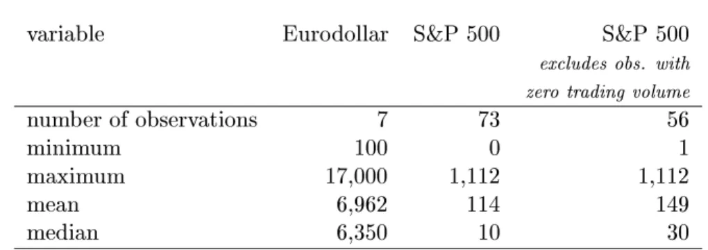
Table 2 presents some summary statistics on the trading volume for op- tions on the S&P 500 and the Eurodollar March futures traded on February 28, 2001.

The number of options and the average trading volume per op-

8

The put-call parity holds exactly for European options and only approximately for American options. However, our pdf-extraction technique treats all options as if they were European-style, so that, including multiple same-strike options in the data set could still result in numerical failure when the American option prices do not verify the put-call parity.

9

This day is chosen as an example. The trading volume patterns that day are fairly

tion greatly dier across underlying assets. The S&P 500 futures support the most options (73), about ten times as many as the Eurodollar futures (7). The average trading volume, in number of contracts, is higher for op- tions on the Eurodollar than on the S&P 500 futures (but the average price of options on Eurodollar futures is lower than that of options on S&P 500 futures). Trading activity is low or nil for many options on S&P 500 futures.

About 23 per cent of the options on S&P 500 futures have zero volume, and, in total, about half of the options have trading volumes of 10 contracts or less, a trading volume more than 10 times lower than the mean. In contrast, none of the options on Eurodollar futures used in the paper has zero volume.

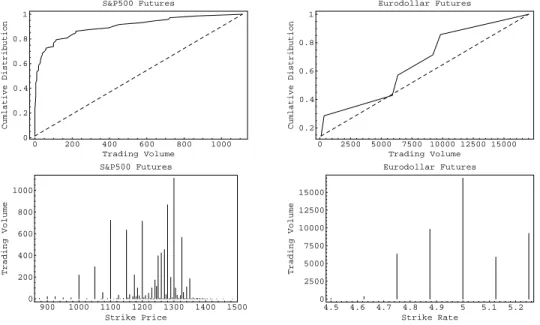
Figure 3 shows the cumulative distribution of trading volume and the trading volume per strike for options on S&P 500 futures and Eurodollar futures. The distance between the distribution function and the diagonal line (which joins the lowest to the highest trading volumes) measures the concentration of the trading volume because the cumulative distribution function of a uniformly distributed random variable would coincide with the diagonal line. Extreme volumes dominate the distribution of trading volume on S&P 500 futures options whereas that on Eurodollar futures options is more balanced.

Although, low volumes tend to be more frequent at strikes farther away from the heart of the distribution, low volumes can occur at any strike (as shown by the options on S&P 500 futures) and strikes in the tail of the distribution can support high trading volumes (as shown by the options on Eurodollar futures). This conrms the idea of this paper that one should take into account trading volume option by option and not merely select options according to their moneyness.

4.2 Results

The following section presents the results of extracting risk-neutral proba- bility distributions alternatively striving to perfectly replicate the market prices of the derivatives on the underlying asset and being satised with only an approximate t, a choice that allows the use of the options' trading volumes to weight their prices.

Implied pdf perfectly replicating the option prices

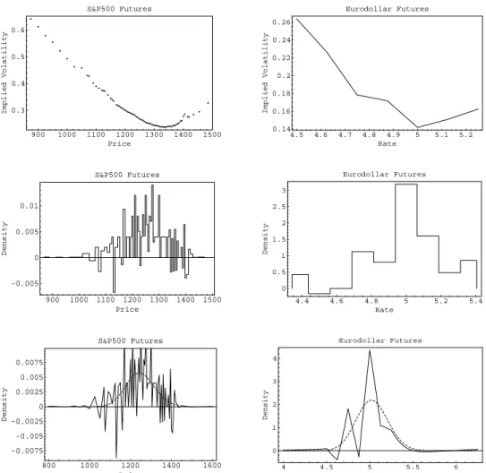
Figure 4 shows the implied volatilities and the implied probability distri- butions using the buttery-spread method and the implied-tree method ob- tained from options on S&P 500 and Eurodollar futures. The high proportion of zero-volume quotes in S&P 500 futures options does not seem to aect the overall smoothness of the smile, suggesting that zero-volume quotes may be the results of interpolating the smile or the option prices.

The implied probability distributions in Figure 4 are designed to per- fectly match the market prices of the options and no positivity constraint is

representative of those on other days. Statistics below pertain to data excluding options

whose prices coincide with their lower bounds and options with a lower trading volume

than options with identical strike and maturity.

imposed. The implied pdf obtained using the buttery method on the S&P 500 futures options shows multiple local peaks and troughs and is sometimes negative. The implied probabilities are negative when a triplet of consecutive option prices is not convex in the strike price. Hence, the implied buttery distribution would not perfectly replicate the market prices of the options if positivity constraints were imposed. Introducing more states of the world than derivatives assets and letting the probability distribution be close to a reference probability distribution while striving to match exactly the option prices|the principle behind the implied-tree method|does not improve the shape of the implied pdf obtained from options on S&P 500 futures. Every spike in the buttery-spread pdf is matched by a spike in the implied-tree pdf of similar or greater magnitude (the vertical axis in the graph in the lower panel is truncated). Imposing positivity constraints, if possible, would only hide the basic fact that some triplets of option prices are not convex in the strike price.

Using the buttery method to construct the implied probability distribu- tion yields better results when dealing with options on Eurodollar futures.

However, the implied-tree method assigns negative implied probabilities to regions where the buttery-spread probabilities were positive. Imposing non- negativity constraints would address this problem. The advantage of the implied-tree method is that it allows extending the support of the distribu- tion further in the tails. In the buttery-spread framework, the probabili- ties of the lowest and the highest possible values of the underlying asset are qualitatively dierent from the other implied probabilities because these two probabilities measure the probability mass in the tails. In this regard, the pickup in the implied pdf at both ends of the Eurodollar rate range suggests that the Eurodollar rate at expiry is likely to equal values outside this range.

The implied-tree method spreads the probability mass over a greater range of values of the Eurodollar rate and yields longer and thinner tails. In this region, the constraint that the implied pdf be close to a reference pdf sig- nicantly aects the implied probability distribution because of the relative paucity of option data in the tails.

Alternative to the implied-tree method

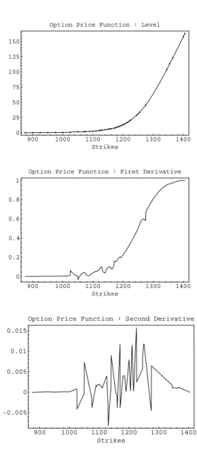
Instead of implied trees, one could use the method of Breeden and Litzen- berger (1978), summarized in Eq. (9), on previously smoothed option prices.

Figure 5 shows the result of tting a smooth function through the prices of

all put options on the S&P 500 futures and taking the rst and the second

derivatives of this function. As shown in the upper panel, the interpolation

scheme delivers an apparently increasing and convex function. However, as

shown in the lower panels, deviations from monotonicity and convexity that

are barely visible in the top panel translate into slight bumps in the rst

derivative and much sharper spikes in the second derivative. Choosing a

cubic spline for the option-price function like in Figure 5|an interpolat-

ing function that is cubic on the segments between two strikes and passes

smoothly through the market prices of the options| results in linear second

derivatives and coincides with the buttery spread in the heart of the distri-

bution. Choosing a higher order for the polynomial interpolating function often results in even more pronounced swings in the second derivatives. In- creasing the order of the interpolating polynomial may allow the imposition of smoothness conditions on the second derivative of the price function at every strike but typically causes the second derivative function to behave erratically between some strikes.

Shimko (1993) and Campa et al. (1997) t the implied volatilities using a polynomial function of the strike price. We do not apply their methods to our data because the volatility smile obtained from options on the S&P 500 futures is even less smooth than the put price function in Figure 5.

More generally, interpolation schemes that work well on data set of small size and good quality may deliver less acceptable results when applied to more numerous and lower-quality data. One may suspect that some options on S&P 500 futures with consecutive strikes correspond to transactions that occurred at dierent times over the trading day. A way of improving the quality of our end-of-day data would be to lter out options that most likely traded at a dierent time than the others. Trading volume can be used as such a lter when no information on transaction time is available.

The undesirable behavior of the pdf also seems to be due more to the constraint of replicating the price of every option than to the selected in- terpolation scheme. To remedy this, one could smooth the prices of the options using a spline with fewer knot points than option prices and obtain the implied pdf by taking the second derivative of this function (and scaling results by exp(

r )). The procedure is simple but the resulting pdf depends on the order of the polynomial used and on the choice of knot points. Those willing to forgo the perfect replication of the market prices of the options may prefer the method outlined in the paper (where a non-matching cost replaces the requirement to perfectly recover the option prices) because of the greater transparency between the parameters (the weight aected to the non-matching cost, etc.) and the resulting pdf.

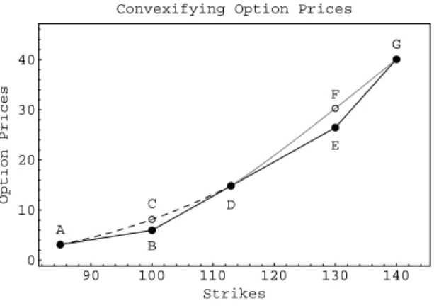
Deleting from the data the observations that cause the price of the op- tions not to be convex in the strike price, or slightly modifying the data to convexify the option prices, would guarantee the non-negativity of the implied probabilities when the buttery spread is used and diminish the likelihood of negative probabilities when the implied tree method is cho- sen. However, as shown in Figure 6, there is no unique way to select the data to make the call price a convex function of the strike price because the buttery-spread based implied probability at any point in the asset-price range depends on the price of three options. In Figure 6, the prices of the put options, represented by the dots joined by the solid line, do not dene a convex function of the strikes, because a line joining points B and E would pass below D. This can be remedied by pulling down D, shifting up B or E, for example towards C and F, respectively, or deleting B or E altogether and using A or G instead in the buttery spread. Each of these choices results in a dierent implied probability distribution.

Implied pdf imperfectly replicating the option prices

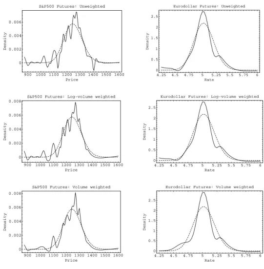
The eect of not requiring the implied distribution to perfectly match the market prices of the options and of weighting each option price by a func- tion of its trading volume is shown in Figure 7. The upper panels show the implied probability distribution when only an approximate t with the option prices is acceptable and every option price has the same weight. The constraint that the implied pdf replicate the market prices of the option is more signicantly lessened for options on S&P 500 futures than for those on Eurodollar futures to insure a relatively smooth pdf for the S&P 500.

The weight on the cost of non matching (

in equation (19)) is 0.5 for the S&P 500 futures options but 0.98 for Eurodollar futures options. However, weights on the non-matching cost are not directly comparable across dier- ent types of assets. For example, there are more options on the S&P 500 futures than on the Eurodollar futures, and hence relatively more probable discrepancies between the market prices of the options and those implied by the pdf. Even with the lessened matching constraint, the pdf obtained from the S&P 500 futures options is fairly erratic. Using trading volume to weight each option price smoothes some of the wiggles, especially when the level of the trading volume is used instead of its logarithm. The pdf obtained from options on Eurodollar futures is hardly aected by weighting each option by the logarithm of its trading volume but is signicantly smoother when the level of the trading volume is chosen.

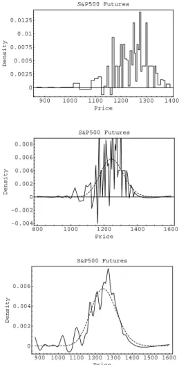
The two weighting schemes used aect options with zero trading volume a zero weight. Figure 8 shows the implied pdfs based on options on S&P 500 futures excluding zero-volume options while aecting the same weight to all remaining options, whatever their trading volumes. The implied pdfs are computed using the buttery spread method, the implied-tree method im- posing a perfect match with the option prices, and the implied-tree method requiring only a partial match with those prices (the weight on the non- matching cost is unchanged). Methods with perfect match results in wiggly and sometimes negative pdfs while relaxing this constraint improves the smoothness of the implied pdf. Weighting each observation by its trading volume improves further the smoothness of the pdf.

The improvement in the overall smoothness of the implied probability distribution does not come at signicant costs for the t between the implied distribution and the market prices of the derivatives. For options on the Eurodollar futures, the mean absolute deviation between the prices implied by the distribution and those observed in the market is about $11 when a lognormal distribution is tted to the option prices, $4 when the implied-tree with imperfect matching but no volume-weighting is used, and $5 when the volume-weighting scheme is used. The respective gures for options on S&P 500 futures are $633, $7 and $9.

10

Options and futures used in the paper are quoted in "points" and 1 point is worth

$25 for derivatives on the Eurodollar and $2.5 for those on the S&P 500 index. The mean

prices are $54 for options on the Eurodollar futures and $2,257 for options on the S&P

500 futures. The sample excludes options whose prices equal their lower bounds or with

zero trading volume. When both a call and a put option are traded at a given strike, the

option with the highest trading volume is selected.

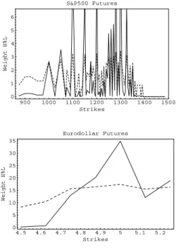
The weighting scheme as bandwidth

As shown in Figure 7, choosing the logarithm or, alternatively, the level of the trading volume of each option signicantly impacts the implied pdf.

Weighting the option prices by the logarithm of the trading volume has roughly the same result as not weighting the option prices at all for options on Eurodollar futures but has a signicant eect for options on the S&P 500 futures. Figure 9 shows the weights on the options for both underlying as- sets. Choosing to weight the option prices by the logarithm of their trading volume limits the inuence of high trading volumes. It nearly aects each option on Eurodollar futures the same weight but preserves some variation across weighted traded volumes for options on S&P 500 futures, while still signicantly reducing the weight of highly traded options. Figure 9 suggests that it is advisable to graph the weight given to each option by potential weighting schemes before computing implied pdfs. As shown in Figure 10, which displays the relative weights as functions of the option's trading vol- ume when the weights are based on the level and on the logarithm of trading volume, the weights based on the logarithm of the trading volume atten out as soon as trading volume increases away from zero so that this weight- ing scheme diers little from not weighting the options. (Trading volume is assumed to be uniformly distributed across strikes, so that the cumulative probability distribution of the trading volume is the 45-degree line.) The volume-based weighting scheme plays a role somewhat similar to that of the bandwidth in a kernel regression. Favoring options with high trading vol- ume reduces the eective number of options used to compute the implied pdf; weighting options more equally includes less relevant data.

5 Conclusion

The paper presents a new way of inferring the probability distribution of an asset from the prices of derivatives based on this asset. The approach recognizes that market prices of options and futures are inherently noisy and introduces two changes. First, instead of requiring that the implied proba- bility distribution perfectly replicate the market prices of the derivatives, the new procedure only imposes a cost of non-matching those prices. Second, it uses trading volume as an indicator of how relevant the price data are and weight each option by a function of its trading volume.

The user selects such a function according to how much he wants to fa- vor high-volume options against low-volume options in the weighting scheme.

Comparing the implied probability distributions obtained with the new method to those obtained using the buttery-spread or the implied-tree methods re- veals signicant improvements in the degree of smoothness of the distribu- tions with a minimal deterioration of the t between the derivatives prices obtained from the implied probability distributions and the corresponding market prices.

Although we only use the trading volume-weighting scheme to implied

trees, the method can be applied to any other technique mapping market

quotes on derivatives contracts to the risk-neutral probability distribution of

the underlying asset. Computational changes are minimal and trading vol-

ume data are as easily available as price data. Users of parametric methods

do not even need to consider the appropriate weight on the non-matching

cost to be able to use trading volume to weight option prices because para-

metric methods typically cannot replicate observed option prices. (In con-

trast, when perfect replication of the option prices is possible, one needs to

loosen the matching constraint for a weighting scheme on the option prices

to make any dierence.) Weighting each option by its trading volume could

reduce the problems linked with overtting the data and produce implied

probability distributions that are both smoother and more reective of fun-

damentals.

Appendix

A Retrieving risk-neutral distributions when there are as many marketable assets as states of the world

Setting the number of states of the world equal to the number of assets and ignoring the positivity constraint on the risk-neutral probabilities, one can easily recover the (unique) risk-neutral probability distribution. From Eq.

(5), it follows that

8

<

:

S i = S

+ ( i

1) for i = 1 :::;n;

K j = K

+ ( j

1) for j = 1 :::;m;

S i

K j = ( i

1

j ) : ⁽²²⁾ Consequently, Eq. (3) is equivalent to

8

<

:

P

m i

( i

1) p i = ( F

S

) = ;

P

m

i

max(0 ;i

1

j ) p i = e ^r C ( K j ) = ;

P

m i

p i = 1 : ⁽²³⁾

Eq. (23) is equivalent to

A:P = Z (24)

with the components of A and Z given by

8

>

>

>

>

<

>

>

>

>

:

a j;i = max(0 ;i

j ) for j = 1 ;:::;m + 1 ;i = 1 ;:::;m + 2 ; a m

;i = 1 for i = 1 ;:::;m + 2 ;

z

= ( F

S

) = ;

z j = e ^r C ( K j

) = for j = 2 ;:::;m + 1 ; z m

= 1 :

(25) A

= B with the components of B equal to 0 except

8

>

>

<

>

>

:

b

;

=

1 ; b

;

= 1 ; b

;m

= 1 ;

b i;i

= 1 ; b i;i =

2 ; b i;i

= 1 for i = 2 ;:::;m;

b m

;m = 1 ; b m

;m

=

2 ;

b m

;m

= 1 : ⁽²⁶⁾

To prove that B :A is the identity matrix, let c i;j =

^m _k

b i;k a k;j and show that c i;j = 1 if i = j and 0 otherwise.

1. Case 2

i

m :

For 2

i

m , b i;m

= 1 if i = 1 and b i;m

= 0 if i

2 and for k

m + 1, a k;j = max(0 ;j

k ). Hence,

c i;j =

^m _k

b i;k a k;j ;

= max(0 ;j

i + 1)

2max(0 ;j

i ) + max(0 ;j

i

1) :

(27)