Text categorization with support vector machines

UNIVERSITAT DORTMUND

Fachbereich Informatik Lehrstuhl VIII

Kunstliche Intelligenz

Text Categorization with Support Vector

Machines: Learning with Many Relevant Features

LS{8 Report 23

Thorsten Joachims

Dortmund, 27. November, 1997 Revised: 19. April, 1998

Universitat Dortmund

Fachbereich Informatik University of Dortmund

Computer Science Department

Forschungsberichte des Lehrstuhls

(KI) Research Reports of the unit no.

(AI)

Fachbereich Informatik Computer Science Department

der Universitat Dortmund of the University of Dortmund

ISSN 0943-4135 Anforderungen an:

Universitat Dortmund Fachbereich Informatik Lehrstuhl

D-44221 Dortmund

ISSN 0943-4135 Requests to:

University of Dortmund Fachbereich Informatik Lehrstuhl

D-44221 Dortmund e-mail: reports@ls8.informatik.uni-dortmund.de

ftp: ftp-ai.informatik.uni-dortmund.de:pub/Reports

www: http://www-ai.informatik.uni-dortmund.de/ls8-reports.html

Machines: Learning with Many Relevant Features

LS{8 Report 23

Thorsten Joachims

Dortmund, 27. November, 1997 Revised: 19. April, 1998

Universitat Dortmund

Fachbereich Informatik

Abstract

This paper explores the use of Support Vector Machines (SVMs) for learning text classi-

ers from examples. It analyzes the particular properties of learning with text data and

identies, why SVMs are appropriate for this task. Empirical results support the theoret-

ical ndings. SVMs achieve substantial improvements over the currently best performing

methods and they behave robustly over a variety of dierent learning tasks. Furthermore,

they are fully automatic, eliminating the need for manual parameter tuning.

1

1 Introduction

With the rapid growth of online information, text categorization has become one of the key techniques for handling and organizing text data. Text categorization is used to classify news stories [Hayes and Weinstein, 1990] [Masand et al., 1992], to nd interesting information on the WWW [Lang, 1995] [Balabanovic and Shoham, 1995], and to guide a users search through hypertext [Joachims et al., 1997]. Since building text classiers by hand is dicult and time consuming, it is desirable to learn classiers from examples.

In this paper I will explore and identify the benets of Support Vector Machines (SVMs) for text categorization. SVMs are a new learning method introduced by V. Vap- nik [Vapnik, 1995] [Cortes and Vapnik, 1995] [Boser et al., 1992]. They are well founded in terms of computational learning theory and very open to theoretical understanding and analysis.

After reviewing the standard feature vector representation of text (section 2.1), I will identify the particular properties of text in this representation in section 2.3. I will ar- gue that support vector machines are very well suited for learning in this setting. The empirical results in section 5 will support this claim. Compared to state-of-the-art meth- ods, SVMs show substantial performance gains. Moreover, in contrast to conventional text classication methods SVMs will prove to be very robust, eliminating the need for expensive parameter tuning.

2 Text Classication

The goal of text categorization is the classication of documents into a xed number of predened categories. Each document d can be in multiple, exactly one, or no category at all. Using machine learning, the objective is to learn classiers from examples which do the category assignments automatically. This is a supervised learning problem. To facilitate eective and ecient learning, each category is treated as a separate binary classication problem. Each such problem answers the question, whether a document should be assigned to a particular category or not.

2.1 Representing Text

The representation of a problem has a strong impact on the generalization accuracy of a learning system. Documents, which typically are strings of characters, have to be trans- formed into a representation suitable for the learning algorithm and the classication task.

IR research suggests that word stems work well as representation units and that their or- dering in a document is of minor importance for many tasks. The word stem is derived from the occurrence form of a word by removing case and ection information [Porter, 1980]. For example \computes", \computing", and \computer" are all mapped to the same stem \comput". The terms \word" and \word stem" will be used synonymously in the following.

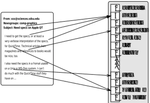
This leads to an attribute-value representation of text. Each distinct word w

corre-

sponds to a feature with TF ( w

;d ), the number of times word w

occurs in the document

d , as its value. Figure 1 shows an example feature vector for a particular document. To

2 2 TEXT CLASSIFICATION

graphics baseball specs

references hockey car clinton

unix space quicktime computer .. . 0 3 0 1 0 0 0

1 0 2 0

From: xxx@sciences.sdsu.edu Newsgroups: comp.graphics Subject: Need specs on Apple QT

I need to get the specs, or at least a

for QuickTime. Technical articles from

be nice, too.

have on ...

very verbose interpretation of the specs,

on a Unix or MS-Dos system. I can’t do much with the QuickTime stuff they I also need the specs in a fromat usable magazines and references to books would

Figure 1: Representing text as a feature vector.

avoid unnecessarily large feature vectors words are considered as features only if they oc- cur in the training data at least 3 times and if they are not \stop-words" (like \and", \or", etc.).

Based on this basic representation it is known that scaling the dimensions of the feature vector with their inverse document frequency IDF ( w

) [Salton and Buckley, 1988] leads to an improved performance. IDF ( w

) can be calculated from the document frequency DF ( w

), which is the number of documents the word w

occurs in.

IDF ( w

) = log

n DF ( w

)

(1) Here, n is the total number of training documents. Intuitively, the inverse document frequency of a word is low if it occurs in many documents and is highest if the word occurs in only one. To abstract from dierent document lengths, each document feature vector

~d

is normalized to unit length.

2.2 Feature Selection

In text categorization one is usually confronted with feature spaces containing 10000 di- mensions and more, often exceeding the number of available training examples. Many have noted the need for feature selection to make the use of conventional learning meth- ods possible, to improve generalization accuracy, and to avoid \overtting" (e.g. [Yang and Pedersen, 1997][Moulinier et al., 1996]).

The most popular approach to feature selection is to select a subset of the available fea-

tures using methods like DF-thresholding [Yang and Pedersen, 1997], the

-test [Sch}utze

et al., 1995], or the term strength criterion [Yang and Wilbur, 1996]. The most commonly

used and often most eective [Yang and Pedersen, 1997] method for selecting features is

the information gain criterion. It will be used in this paper following the setup in [Yang

and Pedersen, 1997]. All words are ranked according to their information gain. To select

a subset of f features, the f words with the highest mutual information are chosen. All

other words will be ignored.

2.3 Why Should SVMs Work Well for Text Categorization? 3

0 20 40 60 80 100

0 1000 2000 3000 4000 5000 6000 7000 8000 9000

Precision/Recall-Breakeven Point

Features ranked by Mutual Information

Bayes Random

Figure 2: Learning without using the \best" features.

2.3 Why Should SVMs Work Well for Text Categorization?

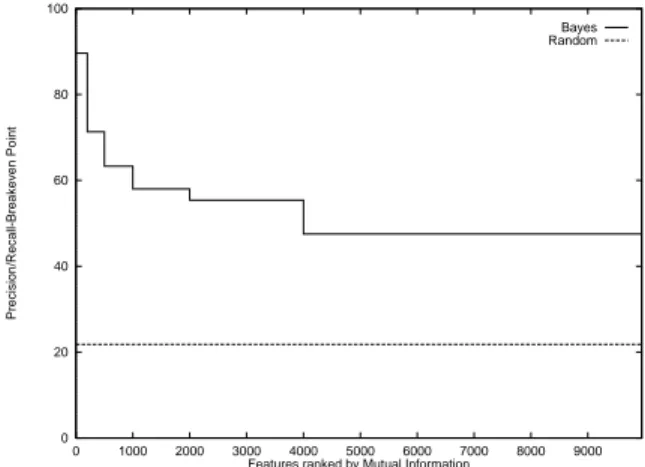
To nd out what methods are promising for learning text classiers, we should nd out more about the properties of text.

High dimensional input space: When learning text classiers on has to deal with very many (more than 10000) features. Since SVMs use overtting protection which does not necessarily depend on the number of features, they have the potential to handle these large feature spaces.

Few irrelevant features: One way to avoid these high dimensional input spaces is to assume that most of the features are irrelevant. Feature selection tries to determine those. Unfortunately, in text categorization there are only very few irrelevant fea- tures. Figure 2 shows the results of an experiment on the Reuters \acq" category (see section 5.1). All features are ranked according to their (binary) mutual infor- mation. Then a naive Bayes classier (see 4.1) is trained using only those features ranked 1-200, 201-500, 501-1000, 1001-2000, 2001-4000, 4001-9947. The results in gure 2 show that even features ranked lowest still contain considerable information and are somewhat relevant. A classier using only those \worst" features has a per- formance much better than random. Since it seems unlikely that all those features are completely redundant, this leads to the conjecture that a good classier should combine many features (learn a \dense" concept) and that feature selection is likely to hurt performance due to a loss of information.

Document vectors are sparse: For each document d

, the corresponding document vector ~d

contains only few entries which are not zero. Kivinen et al. [Kivinen et al., 1995] give both theoretical and empirical evidence for the mistake bound model that \additive" algorithms, which have a similar inductive bias like SVMs, are well suited for problems with dense concepts and sparse instances.

Most text categorization problems are linearly separable: All Ohsumed categories

4 3 SUPPORT VECTOR MACHINES are linearly separable and so are many of the Reuters (see section 5.1) tasks. Insep- arability on some Reuters categories is often due to dubious documents (containing just the words \blah blah blah" in the body) or obvious misclassications of the human indexers. The idea of SVMs is to nd such linear (or polynomial, RBF, etc.) separators.

These arguments give evidence that SVMs should perform well for text categorization.

3 Support Vector Machines

Support vector machines are based on the Structural Risk Minimization principle [Vapnik, 1995] from computational learning theory. The idea of structural risk minimization is to nd a hypothesis h for which we can guarantee the lowest true error. The true error of h is the probability that h will make an error on an unseen and randomly selected test example. The following upper bound connects the true error of a hypothesis h with the error of h on the training set and the complexity of h [Vapnik, 1995].

P ( error ( h ))

train error ( h ) + 2

s

d ( ln

+ 1)

ln

n ⁽²⁾

The bound holds with probability at least 1

. n denotes the number of training examples and d is the VC-Dimension (VCdim) [Vapnik, 1995], which is a property of the hypothesis space and indicates its expressiveness. Equation (2) reects the well known trade-o between the complexity of the hypothesis space and the training error. A simple hypothesis space (small VCdim) will probably not contain good approximating functions and will lead to a high training (and true) error. On the other hand a too rich hypothesis space (high VCdim) will lead to a small training error, but the second term in the right hand side of (2) will be large. This situation is commonly called \overtting". We can conclude that it is crucial to pick the hypothesis space with the \right" complexity.

In Structural Risk Minimization this is done by dening a structure of hypothesis spaces H

, so that their respective VC-Dimension d

increases.

H

H

H

:::

H

::: and

i : d

d

(3) The goal is to nd the index i

for which (2) is minimum.

How can we build this structure of increasing VCdim? In the following we will learn linear threshold functions of the type:

h ( ~d ) = sign

~w

~d + b

=

(

+1 ; if ~w

~d + b > 0

;

1 ; else (4)

Instead of building the structure based on the number of features using a feature selection strategy

, Support vector machines uses a rened structure which acknowledges the fact that most features in text categorization are relevant.

1Remember that linear threshold functions withⁿfeatures have a VCdim ofⁿ+ 1.

5

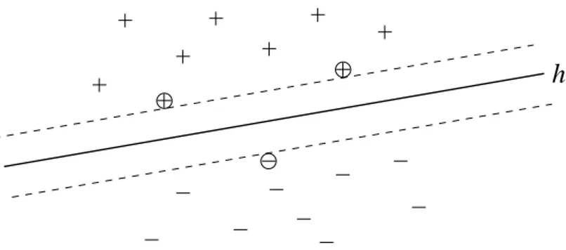
h

Figure 3: Support vector machines nd the hyperplane h , which separates the positive and negative training examples with maximum margin. The examples closest to the hyperplane are called Support Vectors (marked with circles).

Lemma 1. [Vapnik, 1982] Consider hyperplanes h ( ~d ) = sign

~w

~d + b

as hypotheses.

If all example vectors ~d

are contained in a ball of radius R and it is required that for all examples ~d

j

~w

~d

+ b

1, with

~w

= A (5) then this set of hyperplane has a VCdim d bounded by

d

min ([ R

A

] ;n ) + 1 (6)

Please note that the VCdim of these hyperplanes does not necessarily depend on the number of features! Instead the VCdim depends on the Euclidean length

~w

of the weight vector ~w . This means that we can generalize well in high dimensional spaces, if our hypothesis has a small weight vector.

In their basic form support vector machines nd the hyperplane that separates the training data and which has the shortest weight vector. This hyperplane separates positive and negative training examples with maximum margin. Figure 3 illustrates this. Finding this hyperplane can be translated into the following optimization problem:

Minimize:

~w

(7)

so that:

i : y

[ ~w

~d

+ b ]

1 (8) y

equals +1 (

1), if document d

is in class + (

). The constraints (8) require that all training examples are classied correctly. We can use the lemma from above to draw conclusions about the VCdim of the structure element that the separating hyperplane comes from. A bound similar to (2) [Shawe-Taylor et al., 1996] gives us a bound on the true error of this hyperplane on our classication task.

Since the optimization problem from above is dicult to handle numerically, Lagrange multipliers are used to translate the problem into an equivalent quadratic optimization problem [Vapnik, 1995].

Minimize:

i=1

+ 12

y

y

~d

~d

(9)

6 3 SUPPORT VECTOR MACHINES so that:

i=1

y

= 0 and

i :

0 (10) For this kind of optimization problem ecient algorithms exist, which are guaranteed to nd the global optimum

. The result of the optimization process is a set of coecients

for which (9) is minimum. These coecients can be used to construct the hyperplane fullling (7) and (8).

~w

~d = (

i=1

y

~d

)

~d =

i=1

y

( ~d

~d ) and b _{= 12(} ~w

~d

+ ~w

~d

) (11) Equation (11) shows that the resulting weight vector of the hyperplane is constructed as a linear combination of the training examples. Only those examples contribute for which the coecient

is greater than zero. Those vectors are called Support Vectors. In gure 3 the support vectors are marked with circles. They are those training examples which have minimum distance to the hyperplane. To calculate b , two arbitrary support vectors ~d

and ~d

(one from the class + and one from

) can be used.

3.1 Non-linear Hypothesis Spaces

To learn nonlinear hypotheses, SVMs make use of convolution functions K ( ~d

; ~d

). De- pending on the type of convolution function, SVMs learn polynomial classiers, radial basis function (RBF) classiers, or two layer sigmoid neural nets.

K

( ~d

; ~d

) = ( ~d

~d

+ 1)

(12) K

( ~d

; ~d

) = exp ( ( ~d

~d

)

) (13) K

( ~d

; ~d

) = tanh ( s ( ~d

~d

) + c ) (14) These convolution functions satisfy Mercer's Theorem (see [Vapnik, 1995]). This means that they compute the inner product of vectors ~d

and ~d

after they have been mapped into a new \feature" space by a non-linear mapping :

( ~d

)

( ~d

) = K ( ~d

; ~d

) (15) To use a convolution function, simply substitute every occurrence of the inner product in equations (9) and (11) with the desired convolution function. The support vector machine then nds the hyperplane in the \non-linear" feature space, which separates the training data with the widest margin.

3.2 Finding the Best Parameter Values

With the use of convolution functions, parameters are introduced. For the polynomial convolution this is the degree d , for RBFs it is the variance , etc. How can we pick appropriate values for these parameters automatically? The following procedure [Vapnik,

2For the experiments in this paper a rened version of the algorithm in [Osuna et al., 1997] is used.

It can eciently handle problems with many thousand support vectors, converges fast, and has minimal memory requirements.

3.3 Non-Separable Problems 7 1995] can be used, which is again inspired by bound (2). First train the support vector machine for dierent values of d and/or . Then estimate the VCdim of the hypotheses found using (6) and pick the one with the lowest VCdim.

To compute the length of the weight vector one can use the formula

jj

w

=

i;j²SupportV ectors

y

y

K ( ~d

; ~d

) (16) And since all document vectors are normalized to unit length, it is easy to show that the radius R of the ball containing all training examples is tightly bound by

Polynomial: R

2

1 RBF: R

2(1

exp (

)) (17) Please note that this procedure for selecting the appropriate parameter values is fully automatic, does not look at the test data, and requires no expensive cross-validation.

3.3 Non-Separable Problems

So far it was assumed that the training data is separable without error. What if this is not possible for the chosen hypothesis space? Cortes and Vapnik [Cortes and Vapnik, 1995]

suggest the introduction of slack variables. In this paper a simpler approach is taken.

During the optimization of (9) the values of the coecients

are monitored. Training examples with high

\contribute a lot to the inseparability" of the data. When the value of an

exceeds a certain threshold (here

1000) the corresponding training example is removed from the training set. The SVM is then trained on the remaining data.

4 Conventional Learning Methods

This paper compares support vector machines to four standard methods, all of which have shown good results on text categorization problems in previous studies. Each method represents a dierent machine learning approach: density estimation using a naive Bayes classier, the Rocchio algorithm as the most popular learning method from information retrieval, an instance based k -nearest neighbor classier, and the C4.5 decision tree/rule learner.

4.1 Naive Bayes Classier

The idea of the naive Bayes classier is to use a probabilistic model of text. To make the estimation of the parameters of the model possible, rather strong assumptions are incorporated. In the following, word-based unigram models of text will be used, i.e. words are assumed to occur independently of the other words in the document.

The goal is to estimate Pr(+

d

), the probability that a document d

is in class +. With perfect knowledge of Pr(+

d

) the optimum performance is achieved when d

is assigned to class + i Pr(+

d

)

0 : 5 (Bayes' rule). Using a unigram model of text leads to the following estimate of Pr(+

d

) (see [Joachims, 1997]):

Pr(+

d

) = Pr(+)

Pr( w

+)

Pr(+)

Pr( w

+)

+ Pr(

)

Pr( w

)

(18)

8 5 EXPERIMENTS The probabilities P (+) and P (

) can be estimated from the fraction of documents in the respective category. For Pr( w

+) and Pr( w

) the so called Laplace estimator is used [Joachims, 1997].

4.2 Rocchio Algorithm

This type of classier is based on the relevance feedback algorithm originally proposed by Rocchio [Rocchio, 1971] for the vector space retrieval model [Salton, 1991]. It has been extensively used for text classication.

First, both the normalized document vectors of the positive examples as well as those of the negative examples are summed up. The linear component of the decision rule is then computed as

~w = 1

j

+

X

i²+

~d

¹

j;j X

j^2;

~d

(19)

Rocchio requires that negative elements of the vector w are set to 0. is a parameter that adjusts the relative impact of positive and negative training examples. The performance of the resulting classier strongly depends on a \good" choice of .

To classify a new document d

, the cosine between ~w and ~d

is computed. Using an appropriate threshold on the cosine leads to a binary classication rule.

4.3

-Nearest Neighbors

k -nearest neighbor ( k -NN) classiers were found to show very good performance on text categorization tasks [Yang, 1997] [Masand et al., 1992]. This paper follows the setup in [Yang, 1997]. The cosine is used as a similarity metric. knn ( d

) denotes the indexes of the k documents which have the highest cosine with the document to classify d

.

H

( d

) = sign (

P

i²knn(d⁰)

y

cos( d

;d

)

P

i²knn(d⁰)

cos( d

;d

) ) (20) Further details can be found in [Mitchell, 1997].

4.4 Decision Tree Classier

The C4.5 [Quinlan, 1993] decision tree algorithm is used for the experiments in this paper.

It is the most popular decision tree algorithm and has shown good results on a variety of problem. It is used with the default parameter settings and with rule post-pruning turned on. C4.5 outputs a condence value when classifying new examples. This value is used to compute precision/recall tables (see section 5.2). Previous results with decision tree or rule learning algorithms are reported in [Lewis and Ringuette, 1994] [Moulinier et al., 1996].

5 Experiments

The following experiments compare the performance of SVMs using polynomial and RBF

convolution operators with the four conventional learning methods.

5.1 Test Collections 9

5.1 Test Collections

The empirical evaluation is done on two test collection. The rst one is the Reuters-21578 dataset (http://www.research.att.com/lewis/reuters21578.html) compiled by David Lewis and originally collected by the Carnegie group from the Reuters newswire in 1987. The

\ModApte" split is used leading to a corpus of 9603 training documents and 3299 test documents. Of the 135 potential topic categories only those 90 are used for which there is at least one training and one test example. After stemming and stop-word removal, the training corpus contains 9947 distinct terms which occur in at least three documents. The Reuters-21578 collection is know for a rather direct correspondence between words and categories. For the category \wheat" for example, the occurrence of the word \wheat" in a document is an very good predictor.

The second test collection is taken from the Ohsumed corpus (ftp://medir.ohsu.edu /pub/ohsumed) compiled by William Hersh. Here the connection between words and categories is less direct. From the 50216 documents in 1991 which have abstracts, the rst 10000 are used for training and the second 10000 are used for testing. The classication task considered here is to assign the documents to one or multiple categories of the 23 MeSH \diseases" categories. A document belongs to a category if it is indexed with at least one indexing term from that category. After stemming and stop-word removal, the training corpus contains 15561 distinct terms which occur in at least three documents.

5.2 Performance Measures

Despite theoretical problems and a certain arbitrariness, the Precision/Recall-Breakeven Point is used as a measure of performance to stay (at least to some extend) compatible with previously published results. The precision/recall-breakeven point is based on the two well know statistics recall and precision widely used in information retrieval. Both apply to binary classication problems. Precision is the probability that a document predicted to be in class \+" truly belongs to this class. Recall is the probability that a document belonging to class \+" is classied into this class.

Between high recall and high precision exists a trade-o. All methods examined in this paper make category assignments by thresholding a \condence value". By adjusting this threshold we can achieve dierent levels of recall and precision. The PRR method [Raghavan et al., 1989] is used for interpolation.

Since precision and recall are dened only for binary classication tasks, the results of multiple binary tasks need to be averaged to get to a single performance value for multiple class problems. This will be done using microaveraging [Yang, 1997]. In our setting this results in the following procedure. The classication threshold is lowered simultaneously over all binary tasks

. At each value of the microaveraged precision and recall are computed based on the merged contingency table. To arrive at this merged table, the contingency tables of all binary tasks at are added componentwise.

The precision/recall breakeven point is now dened as that value for which precision and recall are equal. Note that there may be multiple breakeven points or none at all. In the case of multiple breakeven points, the lowest one is selected. In case of no breakeven

3Since cosine similarities are not comparable across classes, the method of proportional assignment [Wiener et al., 1995] is used for the Rocchio algorithm to come up with improved condence values.

10 5 EXPERIMENTS

SVM (poly) SVM (rbf)

d = =

Bayes Rocchio C4.5 k-NN 1 2 3 4 5 0.6 0.8 1.0 1.2

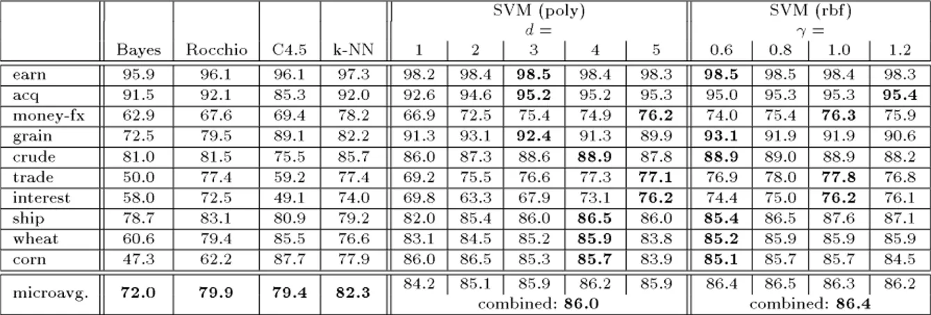
earn 95.9 96.1 96.1 97.3 98.2 98.4 ^98.5 98.4 98.3 ^98.5 98.5 98.4 98.3 acq 91.5 92.1 85.3 92.0 92.6 94.6 ^95.2 95.2 95.3 95.0 95.3 95.3 ^95.4 money-fx 62.9 67.6 69.4 78.2 66.9 72.5 75.4 74.9 ^76.2 74.0 75.4 ^76.3 75.9 grain 72.5 79.5 89.1 82.2 91.3 93.1 ^92.4 91.3 89.9 ^93.1 91.9 91.9 90.6 crude 81.0 81.5 75.5 85.7 86.0 87.3 88.6 ^88.9 87.8 ^88.9 89.0 88.9 88.2 trade 50.0 77.4 59.2 77.4 69.2 75.5 76.6 77.3 ^77.1 76.9 78.0 ^77.8 76.8 interest 58.0 72.5 49.1 74.0 69.8 63.3 67.9 73.1 ^76.2 74.4 75.0 ^76.2 76.1 ship 78.7 83.1 80.9 79.2 82.0 85.4 86.0 ^86.5 86.0 ^85.4 86.5 87.6 87.1 wheat 60.6 79.4 85.5 76.6 83.1 84.5 85.2 ^85.9 83.8 ^85.2 85.9 85.9 85.9 corn 47.3 62.2 87.7 77.9 86.0 86.5 85.3 ^85.7 83.9 ^85.1 85.7 85.7 84.5 84.2 85.1 85.9 86.2 85.9 86.4 86.5 86.3 86.2 microavg. ^{72.0 79.9 79.4 82.3} combined:^86.0 combined:^86.4

Figure 4: Precision/recall-breakeven point on the ten most frequent Reuters categories and microaveraged performance over all Reuters categories. k -NN, Rocchio, and C4.5 achieve highest performance at 1000 features (with k = 30 for k -NN and = 1 : 0 for Rocchio).

Naive Bayes performs best using all features.

point it is dened to be zero.

5.3 Results

Figures 4 and 5 show the results on the Reuters

and the Ohsumed corpus. To make sure that the results for the conventional methods are not biased by an inappropriate choice of parameters, extensive experimentation was done. All four methods were run after selecting the 500 best, 1000 best, 2000 best, 5000 best, (10000 best,) or all features (see section ?? ).

At each number of features the values

0 ; 0 : 1 ; 0 : 25 ; 0 : 5 ; 1 : 0

for the Rocchio algorithm and k

1 ; 15 ; 30 ; 45 ; 60

for the k -NN classier were tried. The results for the parameters with the best performance on the test set are reported.

On the Reuters data the k -NN classier performs best among the conventional methods (see gure 4). This replicates the ndings of [Yang, 1997]. Slightly worse perform the decision tree method and the Rocchio algorithm. The naive Bayes classier shows the worst results. Compared to the conventional methods all SVMs perform better independent of the choice of parameters. Even for complex hypotheses spaces, like polynomials of degree 5, no overtting occurs despite using all 9947 features. This demonstrates the ability of SVMs to handle large feature spaces without feature selection. The numbers printed in bold in gure 4 mark the parameter setting with the lowest VCdim estimate as described in section 3.2. The results show that this strategy is well suited to pick a good parameter setting automatically. Computing the microaveraged precision/recall-breakeven point over the hypotheses with the lowest VCdim per class leads to a performance of 85.6 for the polynomials and 86.3 for the radial basis functions. This is a substantial improvement over the best performing conventional method at its best parameter setting. The RBF

4The results for the Reuters corpus are revised. In the experiments for an earlier version of this report the articles marked with \UNPROC" were parsed in a way that the body was ignored.

11

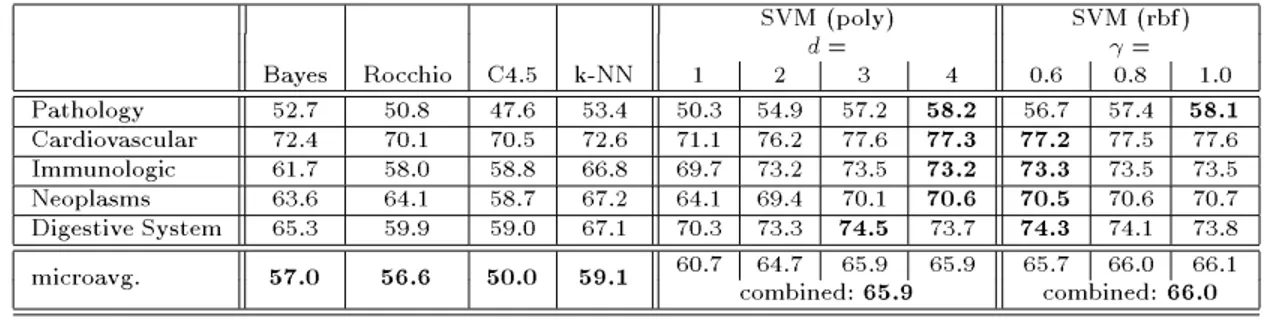
SVM (poly) SVM (rbf)

d = =

Bayes Rocchio C4.5 k-NN 1 2 3 4 0.6 0.8 1.0

Pathology 52.7 50.8 47.6 53.4 50.3 54.9 57.2 ^58.2 56.7 57.4 ^58.1 Cardiovascular 72.4 70.1 70.5 72.6 71.1 76.2 77.6 ^{77.3 77.2} 77.5 77.6 Immunologic 61.7 58.0 58.8 66.8 69.7 73.2 73.5 ^{73.2 73.3} 73.5 73.5 Neoplasms 63.6 64.1 58.7 67.2 64.1 69.4 70.1 ^{70.6 70.5} 70.6 70.7 Digestive System 65.3 59.9 59.0 67.1 70.3 73.3 ^74.5 73.7 ^74.3 74.1 73.8 60.7 64.7 65.9 65.9 65.7 66.0 66.1 microavg. ^{57.0 56.6 50.0 59.1} combined:^65.9 combined:^66.0

Figure 5: Precision/recall-breakeven point on the ve most frequent Ohsumed categories and microaveraged performance over all Ohsumed categories. k -NN, Rocchio, and Bayes achieve highest performance using all features (with k = 45 for k -NN and = 1 : 0 for Rocchio). C4.5 performs best using 500 features.

Support Vector machine is better than k -NN on 62 of the 90 categories (20 ties), which is a signicant improvement according to the binomial sign test.

The results for the Ohsumed collection are similar (gure 5). Again k -NN is the best conventional method. C4.5 fails on this task and heavy overtting is observed when using more than 500 features. Again the SVMs perform substantially better than all other methods. The RBF support vector machine outperforms k -NN on all 23 categories, which is again a signicant improvement. On both the Reuters and the Ohsumed collection the RBF convolution performs slightly better than the polynomial convolution.

Comparing training time, SVMs are roughly comparable to C4.5, but they are more expensive than naive Bayes, Rocchio, and k -NN. Nevertheless, current research is likely to improve eciency of SVM-type quadratic programming problems. SVMs are faster than k -NN at classication time, especially when using the reduced set [Burges and Scholkopf, 1997] method.

6 Conclusions

This paper introduces support vector machines for text categorization. It provides both theoretical and empirical evidence that SVMs are very well suited for text categorization.

The theoretical analysis concludes that SVMs acknowledge the particular properties of text: (a) high dimensional feature spaces, (b) most of the features are relevant (dense concept vector), and (c) sparse instance vectors.

The experimental results show that SVMs consistently achieve good performance on categorization tasks, outperforming existing methods substantially and signicantly. With their ability to generalize well in high dimensional feature spaces, SVMs eliminate the need for feature selection making the application of text categorization considerably easier.

Another advantage of SVMs over the conventional methods is their robustness. SVMs show

good performance in all experiments avoiding catastrophic failure like observed for the

conventional methods on some tasks. Furthermore, SVMs do not require any parameter

tuning, since they can nd good parameter settings automatically. All this makes SVMs

a very promising and easy to use method for learning text classiers from examples.

12 REFERENCES

7 Acknowledgements

Many thanks to my advisor Prof. Morik, Ralf Klinkenberg, and Marc Craven for comments on this paper. Thanks also to Ken Lang for providing some of the code.

References

[Balabanovic and Shoham, 1995] Balabanovic, M. and Shoham, Y. (1995). Learning infor- mation retrieval agents: Experiments with automated web browsing. In Working Notes of the AAAI Spring Symposium Series on Information Gathering from Distributed, Het- erogeneous Environments. AAAI-Press.

[Boser et al., 1992] Boser, B., Guyon, M., and Vapnik, V. (1992). A training algorithm for optimal margin classiers. In Conference on Computational Learning Theory (COLT), pages 144{152.

[Burges and Scholkopf, 1997] Burges, C. and Scholkopf, B. (1997). Improving the accu- racy and speed of support vector machines. In Neural Information Processing Systems, volume 9.

[Cortes and Vapnik, 1995] Cortes, C. and Vapnik, V. (1995). Support-vector networks.

Machine Learning, 20:273{297.

[Hayes and Weinstein, 1990] Hayes, P. and Weinstein, S. (1990). Construe/tis: a system for content-based indexing of a database of news stories. In Annual Conference on Innovative Applications of AI.

[Joachims, 1997] Joachims, T. (1997). A probabilistic analysis of the rocchio algorithm with tdf for text categorization. In International Conference on Machine Learning (ICML).

[Joachims et al., 1997] Joachims, T., Freitag, D., and Mitchell, T. (1997). Webwatcher:

A tour guide for the world wide web. In International Joint Conference on Articial Intelligence (IJCAI).

[Kivinen et al., 1995] Kivinen, J., Warmuth, M., and Auer, P. (1995). The perceptron algorithm vs. winnow: Linear vs. logarithmic mistake bounds when few input variables are relevant. In Conference on Computational Learning Theory.

[Lang, 1995] Lang, K. (1995). Newsweeder: Learning to lter netnews. In International Conference on Machine Learning (ICML).

[Lewis and Ringuette, 1994] Lewis, D. and Ringuette, M. (1994). A comparison of two learning algorithms for text classication. In Third Annual Symposium on Document Analysis and Information Retrieval, pages 81{93.

[Masand et al., 1992] Masand, B., Lino, G., and Waltz, D. (1992). Classifying news

stories using memory based reasoning. In International ACM SIGIR Conference on

Research and Development in Information Retrieval, pages 59{65.

REFERENCES 13 [Mitchell, 1997] Mitchell, T. (1997). Machine Learning. McGraw-Hill.

[Moulinier et al., 1996] Moulinier, I., Raskinis, G., and Ganascia, J. (1996). Text cate- gorization: A symbolic approach. In Annual Symposium on Document Analysis and Information Retrieval (SDAIR).

[Osuna et al., 1997] Osuna, E., Freund, R., and Girosi, F. (1997). An improved training algorithm for support vector machines. In IEEE Workshop on Neural Networks for Signal Processing (NNSP).

[Porter, 1980] Porter, M. (1980). An algorithm for sux stripping. Program (Automated Library and Information Systems), 14(3):130{137.

[Quinlan, 1993] Quinlan, J. R. (1993). C4.5: Programs for Machine Learning. Morgan Kaufmann.

[Raghavan et al., 1989] Raghavan, V., Bollmann, P., and Jung, G. (1989). A critical investigation of recall and precision as measures of retrieval system performance. ACM Transactions on Information Systems, 7(3):205{229.

[Rocchio, 1971] Rocchio, J. (1971). Relevance feedback in information retrieval. In Salton, G., editor, The SMART Retrieval System: Experiments in Automatic Document Pro- cessing, pages 313{323. Prentice-Hall Inc.

[Salton, 1991] Salton, G. (1991). Developments in automatic text retrieval. Science, 253:974{979.

[Salton and Buckley, 1988] Salton, G. and Buckley, C. (1988). Term weighting approaches in automatic text retrieval. Information Processing and Management, 24(5):513{523.

[Sch}utze et al., 1995] Sch}utze, H., Hull, D., and Pedersen, J. (1995). A comparison of classiers and document representations for the routing problem. In International ACM SIGIR Conference on Research and Development in Information Retrieval.

[Shawe-Taylor et al., 1996] Shawe-Taylor, J., Bartlett, P., Williamson, R., and Anthony, M. (1996). Structural risk minimization over data-dependent hierarchies. Technical Report NC-TR-96-053, NeuroCOLT.

[Vapnik, 1982] Vapnik, V. (1982). Estimation of Dependencies Based on Empirical Data.

Springer Series in Statistics. Springer-Verlag.

[Vapnik, 1995] Vapnik, V. (1995). The Nature of Statistical Learning Theory. Springer, New York.

[Wiener et al., 1995] Wiener, E., Pedersen, J., and Weigend, A. (1995). A neural net- work approach to topic spotting. In Annual Symposium on Document Analysis and Information Retrieval (SDAIR).

[Yang, 1997] Yang, Y. (1997). An evaluation of statistical approaches to text categoriza-

tion. Technical Report CMU-CS-97-127, Carnegie Mellon University.

14 REFERENCES [Yang and Pedersen, 1997] Yang, Y. and Pedersen, J. (1997). A comparative study on fea- ture selection in text categorization. In International Conference on Machine Learning (ICML).

[Yang and Wilbur, 1996] Yang, Y. and Wilbur, J. (1996). Using corpus statistics to re-

move redundant words in text categorization. Journal of the American Society for

Information Science, 47(5):357{369.