RESEARCH
Towards individualized cortical thickness assessment for clinical routine
Marlene Tahedl
1,2*Abstract
Background: Cortical thickness measures the width of gray matter of the human cortex. It can be calculated from T1-weighted magnetic resonance images (MRI). In group studies, this measure has been shown to correlate with the diagnosis/prognosis of a number of neurologic and psychiatric conditions, but has not been widely adapted for clinical routine. One of the reasons for this might be that there is no reference system which allows to rate individual cortical thickness data with respect to a control population.
Methods: To address this problem, this study compared different methods to assess statistical significance of cortical thinning, i.e. atrophy. All compared methods were nonparametric and encompassed rating an individual subject’s data set with respect to a control data population. Null distributions were calculated using data from the Human Connectome Project (HCP, n = 1000), and an additional HCP data set (n = 113) was used to calculate sensitivity and specificity to compare the different methods, whereas atrophy was simulated for sensitivity assessment. Validation measures were calculated for the entire cortex (“cumulative”) and distinct brain regions (“regional”) where possible.
Results: The approach yielding the highest combination of specificity and sensitivity implemented generating null distributions for anatomically distinct brain regions, based on the most extreme values observed in the population.
With that method, while regional variations were observed, cumulative specificity of 98.9% and cumulative sensitivity at 80% was achieved for simulated atrophy of 23%.
Conclusions: This study shows that validated rating of individual cortical thickness measures is possible, which can help clinicians in their daily routine to discover signs of atrophy before they become visually apparent on an unpro- cessed MRI. Furthermore, given different pathologies present with distinct atrophy patterns, the regional valida- tion proposed here allows to detect distinct patterns of atrophy, which can further enhance differential diagnosis/
prognosis.
Keywords: Cortical thickness, Neuroimaging, Magnetic resonance imaging (MRI), Individual diagnosis, Atrophy, Neurological assessment
© The Author(s) 2020. This article is licensed under a Creative Commons Attribution 4.0 International License, which permits use, sharing, adaptation, distribution and reproduction in any medium or format, as long as you give appropriate credit to the original author(s) and the source, provide a link to the Creative Commons licence, and indicate if changes were made. The images or other third party material in this article are included in the article’s Creative Commons licence, unless indicated otherwise in a credit line to the material. If material is not included in the article’s Creative Commons licence and your intended use is not permitted by statutory regulation or exceeds the permitted use, you will need to obtain permission directly from the copyright holder. To view a copy of this licence, visit http://creat iveco mmons .org/licen ses/by/4.0/. The Creative Commons Public Domain Dedication waiver (http://creat iveco mmons .org/publi cdoma in/
zero/1.0/) applies to the data made available in this article, unless otherwise stated in a credit line to the data.
Background
Using magnetic resonance imaging (MRI), images with high-tissue contrast [1] of the brain can be acquired with- out making use of radioactive contamination of patients.
Beyond clinical applications, MRI has been widely used
for neuroscientific studies. Constantly, methods are being developed which allow to quantify biologic character- istics of the central nervous system and its constituents more and more differentiated, encompassing blood flow, nerve fiber myelination and properties of the cortex or
“gray matter” (GM). The GM is the location of the neu- ron bodies, whereas the extent of cortical thickness seems to be related to synaptic density, synaptic pruning and intracranial myelination [2–5], rather than the num- ber of neurons [5, 6]. A T1-weighted MRI of the brain is
Open Access
*Correspondence: marlene.tahedl@stud.uni-regensburg.de
1 Department of Psychiatry and Psychotherapy, University of Regensburg, Regensburg, Germany
Full list of author information is available at the end of the article
sufficient to compute cortical thickness in an automated procedure and can be further optimized with an addi- tional T2-weighted image [7,
8]. Common algorithmsto calculate cortical thickness are publicly available, e.g.
under the open-source software package FreeSurfer [9].
Cortical thickness has been subject to a wide range of studies, and cortical thinning (i.e. atrophy) has been associated with diagnosis and progression of a number of neurologic conditions, such as Alzheimer’s Disease [10], Parkinson’s Disease [11] and Multiple Sclerosis [12]
as well as psychiatric conditions, such as depression [13]
and schizophrenia [14]. Interestingly, such pathological conditions present with different patterns of cortical thin- ning and are modified by age and genetic components [15, 16]. These specific aspects make cortical thickness a good candidate as a biomarker for differential diagnosis/
prognosis. However assessing cortical thickness is rarely incorporated in clinical practice. One of the reasons for this might be the lack of a standardized system, based on which an individual’s cortical thickness data can be rated.
To pass this limit, the present study aimed to develop a method to rate an individual’s cortical thickness data with respect to a control population which detects corti- cal atrophy with high sensitivity and specificity. To allow detecting distinct patterns of cortical atrophy, the tested methods allow the evaluation of separate brain regions.
Such a standardized procedure can help clinicians detect early signs of distinct atrophy patterns and monitor their progression.
Methods
SubjectsIn order to rate an individual’s data with respect to a control population, a large number of standardized data from a representative population sample is required.
The Human Connectome Project (HCP) provides such a resource [17–19]. For this study, data from the HCP’s 1200 Subject Release was used. In total, structural data (T1- and T2-weighted sequences) from 1113 subjects was available at the time of this study (507 males, aged between 22 and 40). Of the 1113 subjects, 1000 were randomly selected for generating null distributions of cortical thickness, the rest was spared for subsequent val- idation (see below).
Data acquisition and preprocessing
The HCP data was acquired on a 3 Tesla Connec- tome Scanner. Two different types of structural ses- sions were acquired, encompassing a T1-weighted MPRAGE (repetition time (TR)
= 2400 ms, echo time(TE) = 2.14 ms, inversion time
= 1000 ms, flip angle(FA)
= 8°, field of view (FOV) = 224 × 224, voxel reso-lution (VR)
= 0.7 mm3, bandwidth (BW)
= 210 Hz/Px,iPAT factor 2, total acquisition time 7 min 40 s) and a T2-weighted SPACE (TR
= 3200 ms, TE = 565 ms, FAvariable, FOV
= 224 × 224, VR = 0.7 mm3, BW
= 744 Hz/Px, iPAT factor 2, total acquisition time 8 min 24 s). The full imaging protocols can be found online at http://proto
cols.human conne ctome .org/HCP/3T/imagi ng-proto cols.html. All study procedures of the HCP protocol were
approved by the Institutional Review Board at the Wash- ington University in St. Louis.
The HCP offers data which was preprocessed with standardized and validated procedures. The main pre- processing steps encompassed gradient distortion cor- rection, brain extraction, nonlinear registration, surface registration, and registration onto high-resolution (164 k mesh) and low-resolution (32 k mesh) templates; more details on the exact preprocessing pipeline can be found in [9,
20–22]. The image format of the mesh images isin CIFTI format (Connectivity Informatics Technology Initiative), a file format which combines surface-based cortical data with volumetric-based subcortical/cerebel- lar data, which was found to enhance alignment to the geometry of the cortex as well as statistical power [23].
The HCP’s minimally preprocessed data include corti- cal thickness maps (generated based on the standardized FreeSurfer pipeline with combined T1-/T2-reconstruc- tion [7,
8]). For this study, the high-resolution corticalthickness maps (164 k mesh) were used.
Statistical analysis
Statistical analysis of the minimally preprocessed HCP neuroimaging data was carried out with tools from the Connectome Workbench [18, 19] and MATLAB R2019b (The Mathworks, Natick, USA). First, null distribu- tions were generated using different strategies and sub- sequently, these methods were validated and compared based on their specificity and sensitivity.
Generating null distributions
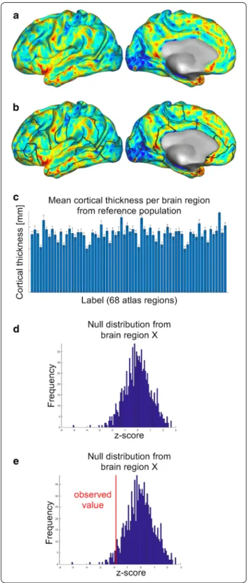
Different strategies to generate null distributions were compared. These can be subdivided into (a) generat- ing one common null distribution for all data points on the cortex (referred to as “vertices” in CIFTI mesh files) and (b) generating separate null distributions for distinct brain regions (Fig.
1a, b). Note that thickness spreadsnonuniformly across the human cortex [24–27] such that different brain regions show different population means (Fig.
1c). Therefore, different null distributions for dis-tinct brain regions might increase sensitivity of detecting atrophy, which is why both approaches were compared in the present study. The two approaches were subdivided further into more and less conservative statistical correc- tions, such that in total, four methods were compared.
Null distributions were computed using nonparametric
permutation procedures for all methods [28], since they make less assumptions than parametric models and are
therefore considered more robust than parametric tests [29, 30].
Method 1: Z‑min statistic per data point
The statistically most conservative approach was based on generating one common reference distribution for all 298,261 data points of the cortical surface. First, from 1000 HCP data sets, each data set was selected iteratively (“test data set”) and standardized with respect to the remaining 999 data sets (“control data sets”). For that, z-scores were calculated for each vertex using the formula z
vertex= (d
vertex– μ
vertex)/
σ
vertex, whereas d
vertexis the cortical thickness value of one vertex from the test data set, μ
vertexthe mean value of that vertex from the control data sets and σ
vertexthe respec- tive standard deviation. From the resulting z-score map, only the minimum value was saved (note that the present research question specifically addresses cortical thinning).
The result was a reference distribution consisting of 1000 z-scores. Using this distribution, each vertex of an inde- pendent validation data set can be rated separately with respect to the reference population, by z-transforming each vertex using the above formula (see section “Valida-
tion”).Method 2: Z‑min statistic per data point, averaged across brain regions
In method 1, a null distribution was calculated based on the most extreme values across the cortex. However, given that cortical thickness is nonuni- formly distributed across the cortex physiologically [27], potential atrophy will be hard to detect in physiologi- cally thicker brain regions. Method 2 aimed to increase the biological plausibility of the previous method. While the same null distribution was used as in method 1, in method 2, data points were summarized across anatomi- cally distinct brain regions, defined by the Desikan–Kil- liany atlas [31]. This atlas subdivides the cortical surface into 68 regions based on morphologic features (“labels”, 34 on each hemisphere). For subsequent validation, sta-
Fig. 1 Generating a reference system for rating an individual’s cortical thickness data with respect to a control population. In methods 3 and 4, each cortical thickness map from a population sample (a) was divided into 68 distinct brain regions (borders are indicated as black lines in b). Given that the different brain regions have different means and standard deviations (c), this approach is biologically more plausible than generating one common reference system for all brain regions (as was tested here in methods 1 and 2).
Based on these null distributions (see d for an example), the observed values for an individual can be rated within the control population (see red line in e) and statistically significant cortical thinning (i.e.
atrophy) can be assessed
▸
tistical significance was determined for the synopsis of all vertices within each of the 68 regions, instead of for each vertex separately (see section “Validation”).
Method 3: Z‑min statistic per brain region
In spite of the increased biological plausibility in method 2, that pro- cedure was still based on one common null distribution from the most extreme values of the cortex. In method 3, this was corrected by calculating distinct null distribu- tions for each of the 68 Desikan–Killiany-labels. For that, the permutation procedure described in method 1 was repeated, however now z-maps were calculated using the formula z
vertex= (dvertex– μ
Label)/σ
Label, whereas z
vertexwas the z-score for a vertex of the test data set, d
vertexis the observed cortical thickness value for that vertex from the test data set, μ
Labelis the mean value of the respective label from the control data sets and σ
Labelits respective stand- ard deviation. On each iteration, the minimum z-score of all vertices composing one common label was saved, such that the result was a 68x1000 matrix, providing a null distribution for each label (Fig. 1d). With these null distributions, each brain region can be rated separately with respect to the reference population, by converting the cortical thickness data into z-scores using the formula z
Label= (d
Label– μ
Label)/σ
Label(Fig. 1e).
Method 4: Z‑score per brain region
Finally, in method 4, null distributions were generated based on averaging
across all vertices from each brain region instead of usingeach label’s most extreme values, as in method 3. Mean values were calculated for each brain region of the test data set to derive null distributions. These null distribu- tions were generated in analogy to method 3, using the formula z
Label= (d
Label– μ
Label)/σ
Label. Similar to method 3, also in method 4, each brain region can be rated sepa- rately with respect to the reference population, by con- verting the cortical thickness data into z-scores using the formula z
Label= (d
Label– μ
Label)/σ
Label.
Validation
To validate and compare the proposed methods, speci- ficity and sensitivity were calculated. These measures were calculated for each vertex (method 1) or each label (methods 2–4) separately. For that, the 113 data sets (“validation data sets”) from the 1113 HCP data sets were used which had been spared for the generation of null distributions (see section “Subjects”). Statistical inference tests based on the null hypothesis of no atro- phy for a given validation data set were carried out using the above-generated null distributions. For each vertex/
label, the number of values of the null distributions that were lower than the observed cortical thickness values in a given validation data set were counted. Dividing this
sum by the number of permutations (n
= 1000) yieldedFWER-corrected p-values (p
FWER) [32,
33]. Vertices/labels with p
FWER<= 0.05 were considered to indicate lower cortical thickness values than would not be pre- dicted by chance and therefore labeled as “atrophic”. In method 2, since data points were summarized within each label, a label was defined as “atrophic” if a certain percentage of its vertices showed p
FWER<= 0.05. Differ- ent percentages were tested (1%, 5%, 10%, 20%, 30%, 40%, 50%). Given that all of these thresholds yielded similarly poor results, hereafter only the results for one threshold (5%, arbitrary choice) are provided. The data for the other thresholds are provided in Additional files 1 and 2.
Specificity
Specificity defines the rate of true negatives, i.e. the share of patients which are correctly diagnosed as not having the condition of interest (here, “no atrophy”).
The validation data set was used to calculate specificity, assuming that—given this data set was a random selec- tion of a data set of healthy young subjects with no his- tory of psychiatric/neurologic disorders—the validation data set can be labeled as non-atrophic. Each of the four methods was applied to all of the 113 validation data sets and specificity was defined as the percentage of vertices (method 1)/labels (methods 2, 3, 4) which were not classi- fied as significantly atrophic. This procedure was repeated for each validation data set separately. Mean and standard deviations of the specificity calculations were determined across all 113 data sets (“cumulative specificity”).
To allow evaluation for distinct brain regions, in addi- tion, specificity per atlas region was defined (for methods 2,3 and 4 only, since in method 1, no atlas regions were analyzed). This was done by calculating, per atlas region, the percentage of the 113 validation data sets which were not significantly classified as atrophic in that atlas region (“regional specificity”).
Sensitivity
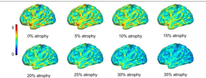
Sensitivity defines the rate of true positives, i.e. the share of patients which are correctly diagnosed as having the condition of interest (here, “atrophy”). Given no true atrophy was assumed in the validation data sets, atrophy was simulated: Different degrees of atrophy were simulated as follows (Fig.
2): The original corticalthickness data (each vertex) was multiplied by a number between 0 and 1 (e.g. multiplication by 0.9 represents simulated atrophy of 10%, etc.). For each of the 113 vali- dation data sets, atrophy was simulated from 1% to 100%
in steps of 1 percentage points (p.p.). Then, each of the four methods was applied to all of the simulated data sets.
For each method and degree of atrophy, sensitivity was
calculated separately. Cumulative sensitivity was defined
as the percentage of vertices (method 1) or labels (meth-
ods 2, 3, 4) which were classified as significantly atrophic,
summarized across all 113 data sets (“cumulative sensi- tivity”). Sensitivity across methods was compared using the degree of atrophy required to achieve cumulative sen- sitivity of 80% (“cumulative sensitivity threshold”). Note that less sensitive methods will require more pronounced atrophy, therefore a higher cumulative sensitivity thresh- old, in order to detect atrophy.
To allow evaluation for distinct brain regions, addi- tionally, sensitivity per atlas region was defined for each degree of atrophy (for methods 2,3 and 4 only, since in method 1, no atlas regions were analyzed). This was done by calculating, per atlas region, the percentage of the 113 validation data sets which were significantly classified as atrophic in that atlas region (“regional sensitivity”).
Note that although cortical thickness was simulated at consistent rates throughout the cortex (which is not how cortical thinning occurs in aging or pathology [10,
15, 16]), evaluation was performed for each vertex/labelindependently. Therefore, the proposed methods are fit to analyze also diffuse patterns of cortical thinning.
Results
SpecificityTable
1 summarizes the cumulative specificity calcula-tions for each method. Methods 1 and 2 showed ideal specificity (100%,
± 0 p.p.), such that these methods clas-sified no vertex (method 1)/label (method 2) as signifi- cantly atrophic. Method 3 had a mean specificity of 98.9%
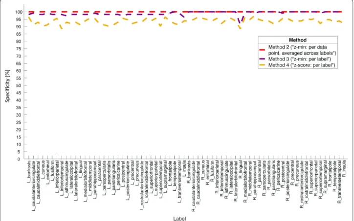
(± 1.3 p.p.), and method 4 was less specific with a mean of 93.6% (± 2.0 p.p.). Figure 3 shows the regional specific- ity profiles evaluated across all 68 atlas regions. While the most specific method (method 2, red dashed line) yielded 100% specificity for each label, method 3 showed rela- tively constant specificity across brain regions except for a slight drop for the right lingual gyrus. Method 3 showed specificity of 100% for almost all labels on the right hemi- sphere (notice however a slight drop for the right lingual gyrus), while the values were slightly lower for the labels on the left hemisphere. Finally, method 4 (golden dashed line) showed notably lower values throughout all labels as compared to methods 2 and 3.
Fig. 2 Atrophy was simulated for sensitivity calculations as follows: The original cortical thickness map from each of the subjects from the control population (“0% atrophy”) was multiplied by values ranging between 0 and 1. Multiplication by lower values indicate higher degrees of simulated atrophy. For example, multiplication by 0.9 simulates 10% atrophy, multiplication by 0.8 20% atrophy, etc. In the present study, atrophy was simulated between 1% and 100% in steps of one percentage points. This allows to assess sensitivity by the degree of simulated atrophy. In this Figure, coloring indicates cortical thickness in millimeters
Table 1 Cumulative specificity calculations for the four tested methods
p.p.: percentage point(s) Method 1 (“z-min:
per data point”)
Method 2 (“z- min: per data point, averaged across labels”)
Method 3 (“z-min:
per label”)
Method 4 (“z-score:
per label”)
Mean specificity (across subjects)
100% 100% 98.9% 93.6%
Standard deviation (across subjects)
0.0 p.p. 0.0 p.p. 1.3 p.p. 2.0 p.p.
Sensitivity
Figure
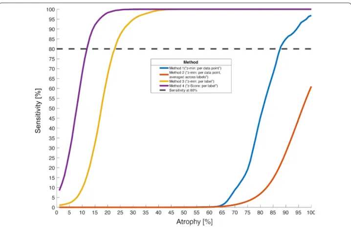
4 illustrates the cumulative sensitivity profiles foreach method relative to the degree of simulated atro- phy. The horizontal dashed line denotes sensitivity at 80% (cumulative sensitivity threshold), which was used to compare the different methods. Table
2 summarizesthese results: Method 1 (red line) was extremely unsensi- tive, such that not even for the highest possible degree of atrophy (literally no brain) did this method detect atro- phy in 80% of cases (i.e. cumulative sensitivity threshold not reached). Method 2 (blue line) yielded a cumulative sensitivity threshold for 88% simulated atrophy when a label was considered atrophic if 5% of its vertices had p
FWER< 0.05 (see “Methods”). Other tested thresholds for method 2 comprised 1% (cumulative sensitivity threshold for 84% simulated atrophy), 10% (90% atrophy), 20% (94%
atrophy), 30% (98% atrophy), 40%/50% (did not reach 80% sensitivity for any degree of simulated atrophy, see Additional file 1: Fig. S1 and Additional file
2: Table S1).Method 3 (yellow line) was clearly superior (cumulative
sensitivity threshold 23% simulated atrophy), and for method 4 an even lower value (12% simulated atrophy) was observed.
Figure
5 shows the results of the regional sensitivitydetermination for methods 2 (Fig.
5a), 3 (Fig. 5b) and 4(Fig.
5c). To compare the methods, the regional sensi-tivity profiles are plotted for each method’s cumulative sensitivity threshold (i.e. 88% atrophy for method 2: blue lines, 23% atrophy for method 3: red lines, 12% atrophy for method 4: golden lines). To enhance orientation, 80%
sensitivity is indicated with a gray dashed line in Fig. 5a–
c. Additionally, regional specificity for each method is plotted (red dashed lines).
Figure 5a illustrates poor sensitivity of method 2, given
it reaches sensitivity of > 0% for none of the cumulative
sensitivity thresholds of the other methods. Additionally,
the regional sensitivity profile for its own cumulative sen-
sitivity threshold (88% simulated atrophy) shows strong
variations across labels. Method 3 (Fig.
5b) is clearlysuperior: while the variations for its own cumulative
Fig. 3 Comparison of regional specificity profiles between methods 2–4. The statistically most conservative approach (method 2, “z-min: per data point, averaged across labels”, red dashed line) yielded ideal specificity for all brain regions, i.e. it correctly assigns “no atrophy” in 100% of cases. The less conservative method 3 (“z-min: per label”, purple dashed line) also showed specificity of 100% for many brain regions, but had some drops, e.g. for the right lingual gyrus. The most liberal approach, method 4 (“z-score: per label”, golden dashed line) yielded lower specificity for all brain regions. Note that method 1 (“z-min: per data point”) is not shown here because it does not allow for labelwise assessment. See also Table 1 for the cumulative specificity values for each methodFig. 4 Cumulative sensitivity relative to the degree of simulated atrophy (across vertices/brain regions), comparison between the four tested methods. All methods detected atrophy more sensitive for more pronounced degrees of atrophy. However, the degree of atrophy the methods required to reach a given level of sensitivity differed. For example, in the current simulation, in order to detect atrophy in 80% of cases (black horizontal dashed line), method 4 (“z-score: per label”, purple line) required only 12% atrophy, method 3 (“z-min: per label”, golden line) 23%, method 2 (“z-min: per data point, averaged across labels”, blue line) 88%, while method 1 (“z-min: per data point”, red line) failed to detect atrophy in 80% of cases even for the highest possible degree of atrophy (100%). Compare also Table 2 for a summary of these results
Table 2 Cumulative sensitivity thresholds for the four tested methods
* Note that lower values of atrophy suggest more sensitive methods, since they detect less pronounced atrophy Method 1 (“z-min: per data
point”) Method 2 (“z-min:
per data point, averaged across labels”)
Method 3 (“z-min:
per label”) Method 4 (“z-score:
per label”)
Degree of atrophy required for detection of atrophy in 80% of cases (cumulative sensitivity threshold)*
Not available 88% 23% 12%
(See figure on next page.)
Fig. 5 Regional sensitivity (per brain region) for each region’s cumulative sensitivity threshold (i.e. the degree of atrophy each method required to detect atrophy in 80% of cases) for method 2 (a, “z-min: per data point, averaged across labels”, method 3 (b, “z-min: per label”) and method 4 (c,
“z-score: per label”). The cumulative sensitivity threshold for method 2 was 88% atrophy (blue lines), for method 3 23% atrophy (red lines) and for method 4 12% atrophy (golden lines). The 80% sensitivity line is indicated by the gray dashed lines in each panel. In addition, regional specificity is plotted for each method (red dashed lines, compare also Fig. 3). All methods detected atrophy more sensitively for more pronounced degrees of atrophy
sensitivity threshold (23% simulated atrophy) are less pronounced as compared to method 2, it yields per- fect (i.e. 100%) sensitivity for the cumulative sensitivity threshold of method 2. However, no region reaches 80%
sensitivity for the cumulative sensitivity threshold of method 3. Finally, method 4 (Fig. 5c) is the most sensitive of the tested methods. It yields almost perfect regional sensitivity for the cumulative sensitivity thresholds of methods 2 and 3, and the regional sensitivity profile for its own cumulative sensitivity threshold (12% simulated atrophy) shows less variations than the other methods.
Note however the relatively low specificity (red dashed line) of this method as compared to the others.
Nevertheless, it is evident from Fig.
5 that thereare regional variations for the cumulative sensitivity thresholds for each method. Additional file 3: Table S2 lists the labels which show less regional sensitivity than 80% for each method and their respective cumu- lative sensitivity threshold. For example, for method 3, among the brain regions that yielded least sensitivity for that method’s cumulative sensitivity threshold (23%
atrophy) are, on the left hemisphere, parahippocam- pal gyrus (49.56% sensitivity), temporal pole (23.89%
sensitivity), frontal pole (9.73% sensitivity), temporal pole (23.89% sensitivity) and transverse temporal gyrus (1.77% sensitivity), and on the right hemisphere, pars orbitalis (27.43% sensitivity), rostral anterior cingulate (24.78% sensitivity), frontal pole (29.20% sensitivity), temporal pole (6.19% sensitivity) and transverse tempo- ral gyrus (23.89% sensitivity).
Discussion
The goal of this study was to develop a method which allows to rate a single patient’s cortical thickness data and identify atrophy sensitively and specifically with respect to a control population. This study was moti- vated by the many previous reports which have found pronounced associations of cortical thinning with the diagnosis/progression of diverse neurological and psy- chiatric conditions. In addition, given that different pathologies present with different patterns of cortical thinning, another goal was to allow the evaluation of cortical thinning for distinct brain regions. To provide such a resource, a reference system was developed by generating population-based distributions of expected cortical thickness data, both for the entire cortex as well as for distinct brain regions. 1000 data sets from young and healthy participants were used to generate expected population null distributions using a per- mutation procedure. To assess statistically significant cortical thinning (i.e. atrophy), different methods were tested and compared using sensitivity and specific- ity calculations for the entire cortex (“cumulative”) as
well as for distinct brain regions (“regional”), calculated from 113 additional subjects. The statistically most stringent methods were based on one common null distribution for all brain regions, which showed ideal specificity but poor sensitivity. Other methods were based on distinct null distributions for different brain regions, which increased sensitivity but decreased specificity. However, when generating distinct null dis- tributions for different brain regions based on the most extreme values within each label (method 3), the drop in cumulative specificity was only very subtle (98.9%), while cumulative sensitivity could still be detected at 80% for 23% simulated atrophy. Variations of regional differences were observed for some brain regions, but decreased for more pronounced degrees of atrophy.
These results emphasize that in order to sensitively detect cortical atrophy for individual patients, it is rea- sonable to create different null distributions for distinct brain regions. Cortical thickness is not spread uniformly across the cortex [34], such that for example neurite den- sity is higher for motor regions as compared to regions associated with higher cognitive functions [27]. There- fore, a single reference distribution to rate any cor- tex region is biologically implausible and will result in decreases of sensitivity, which was shown here in meth- ods 1 and 2. Furthermore, with this approach, sensitivity is relatively constant for different brain regions, although regional variations are observed (Fig. 5b).
One drawback of working with several null distribu- tions for different brain regions as opposed to a com- mon one is that specificity decreases, which was shown in methods 3 and 4. In method 3, a strategy was sug- gested to minimize this loss in specificity while main- taining a high level of sensitivity: The idea of method 3 was to generate null distributions for different brain regions based on the (minimally) most extreme values within each brain region across a control population, instead of working with averages across brain regions.
With this strategy, atrophy could be detected in 80% of
cases when the cortex was roughly three quarters of its
original thickness. However, in cases where the clini-
cian wishes to detect atrophy more sensitively, method
4 might be preferred—there, null distributions were
generated from population averages (rather than from
their most extreme values). In this study, that method
could detect atrophy in 80% of cases already when the
cortex was thinned by a factor of only 12% (also here,
regional variations were observed, see Fig.
5c). How-ever, that approach would imply risking to detect false
positives, given its lower specificity. Depending on the
situation, the clinician can flexibly choose between
more sensitivity or more specificity.
One limitation of the suggested reference system is that it was generated from a relatively homogenous control population of healthy young adults. However, cortical thickness declines even in physiological aging, such that the comparison of an elderly individual to that reference group will result in more pronounced atro- phy detection, which would not necessarily have to be pathologic [10, 15]. Nevertheless, given that the regions that exhibit cortical thinning differ in physiological and pathological aging (for example, atrophy of brain regions such as the precuneus and the inferior tempo- ral region can be indicative of early signs of dementia [35]), it is still possible to detect such potential patho- logic signatures using the method proposed here. This is possible because the reference system suggested herein was generated and evaluated for different brain regions separately. This allows to rate different brain regions independently, such that different atrophy patterns can be identified. Figure
6 illustrates this: For patient X,atrophy was simulated in frontal areas, for patient Y in more posterior regions. Using method 3, the resulting p-map indicates where cortical thinning occurred for that patient. Such maps can be generated easily with a given patient’s T1-weighted MRI using the procedure proposed here, and are therefore easy to implement into clinical practice.
The atlas used in this work was the Desikan–Killiany atlas, a brain atlas defined by morphologic features of the cortex and therefore surface-based. This is an important feature because cortical thinning is modified by genetic components [15,
16], and such genetic pat-terns yield high resemblance to surface-based features [36]. Additionally, patterns of genetic overlap seem to be coarse-grained across the human cortex (current opti- mal solutions suggest between 9 and 12 labels per hemi- sphere [16,
36]), such that the Desikan–Killiany atlas(34 labels per hemisphere) allows a more fine-grained resolution than proposed by genetic commonalities.
However, especially in early pathology, cortical thinning may be more localized, such that future work should investigate the benefit of using a more fine-grained atlas for such cases. Furthermore, a more fine-grained atlas might also help to enhance regional sensitivity of those brain regions which showed poor sensitivity with the Desikan–Killiany altas (such as the left frontal pole as well as the left and right transverse temporal gyri). The evaluation of these regions with the current method and atlas should be made with caution given their lower sensitivity.
Finally, the current reference system allows to pro- gress-monitor an individual’s condition: given the com- position of the reference standard does not change, any potential changes between two measurement time points can be more likely attributed to changes in the individual.
Finally, it should be emphasized that atrophy was only simulated in this study, and it is subject to future work to validate the present simulations with real data. It will also be necessary to show that the system is applicable to data acquired from different types of MR scanners and sequence parameters (here, data from a 3 Tesla MR scan- ner with optimized parameters for T1-weighted imaging were analyzed).
Conclusions
Taken together, the here suggested reference system can be used for sensitive and specific detection of cor- tical atrophy for distinct brain regions (defined by the Desikan–Killiany atlas) for age groups comparable to the reference population (22–40 years), which allows to detect differential patterns of cortical thinning. However, some brain regions are detected less sensitively such that those regions should be evaluated with care. The method should therefore be further validated with data from dif- ferent pathologies and using different atlases. Although distinct reference systems for different age groups will further help to establish this method in clinical practice, the current method already allows to rate elderly individ- uals, however these cases should be treated with caution given the risk of detecting false positives due to effects
Fig. 6 Exemplary result of analyzing a T1-weighted MRI data set withthe current methods. For patient X, cortical thinning was simulated in frontal regions, for patient Y in more posterior regions. Method 3 was used to analyze the data. The emerging p-map indicates where cortical thinning likely occurs in each patient. Using the method proposed in this text, such maps can be created easily and are therefore simple to implement into clinical practice
of physiological aging. However, progress-monitoring of elderly individuals is possible with the current system if the individual is compared to its own ranking within the control population for each measurement time point.
Therefore, the tool proposed in this work represents a first step of the translation of cortical thickness measures into clinical practice.
Supplementary information
Supplementary information accompanies this paper at https ://doi.
org/10.1186/s1296 7-020-02317 -9.
Additional file 1: Figure S1. Cumulative sensitivity relative to the degree of simulated atrophy (across vertices/brain regions), comparison between the four tested methods and different thresholds for method 2. In method 2, a label was defined “atrophic” if a certain percentage of its vertices yielded pFWER <= 0.05. Here, the results for thresholds 1%, 5% (which is shown in the main text), 10%, 20%, 30%, 40% and 50% are displayed Additional file 2: Table S1. Cumulative sensitivity calculations for differ- ent thresholds for method 2 (in method 2, a label was defined “atrophic” if a certain percentage of each label’s vertices yielded pFWER <= 0.05).
Additional file 3: Table S2. For methods 2,3 and 4, cumulative sensitivity was defined based on the degree of simulated atrophy a method required to sensitively detect 80% (method 2: 88% simulated atrophy, method 3: 23% simulated atrophy, method 4: 12% simulated atrophy). However, regional sensitivity varied for that degree of atrophy. This table indicates which labels showed < 80% sensitivity for each method’s “crucial” degree of atrophy, along with the regional sensitivity detected for that degree of atrophy.
Abbreviations
BW: Bandwidth; FA: Flip angle; Fig: Figure; FOV: Field of view; GM: Gray matter;
HCP: Human Connectome Project; MRI: Magnetic resonance imaging; p.p.:
Percentage point(s); TE: Echo time; TR: Repetition time; VR: Voxel resolution.
Acknowledgements
This study was supported by the German Multiple Sclerosis Society (Deutsche Multiple Sklerose Gesellschaft, DMSG) (see “Funding”). Materials and support for the analysis were made available by the Biomedical Imaging Group at the Department of Psychiatry and Psychotherapy, University of Regensburg, Germany, led by Jens V. Schwarzbach, which the author would like to thank.
Authors’ contributions
MT is the sole author of this work. She developed the idea for this work and is responsible for data analysis and statistics, conception of the manuscript, generating figures, tables and any other work related to this manuscript. The author read and approved the final manuscript.
Funding
MT is supported by a grant from the German Multiple Sclerosis Society (Deutsche Multiple Sklerose Gesellschaft, DMSG) (2018_DMSG_08).
Availability of data and materials
All data used in this study are freely and openly available for scientific inter- rogations from the Human Connectome Project. Researchers can access them online at https ://db.human conne ctome .org/app/templ ate/Login .vm;jsess ionid =A3E03 522D3 DEC91 B2D2A 09FB8 0CCE6 CF.
Ethics approval and consent to participate
All study procedures of the Human Connectome Project study protocol were approved by the Institutional Review Board at the Washington University in St. Louis.
Consent for publication
The (sole) author declares her consent for publication.
Competing interests
The author declares no competing or conflicts of interests.
Author details
1 Department of Psychiatry and Psychotherapy, University of Regensburg, Regensburg, Germany. 2 Institute for Experimental Psychology, University of Regensburg, Regensburg, Germany.
Received: 11 February 2020 Accepted: 26 March 2020
References
1. Brant-Zawadzki M, Enzmann DR, Placone RC, Sheldon P, Britt RH, Brasch RC, et al. NMR imaging of experimental brain abscess: comparison with CT. Am J Neuroradiol. 1983;4(3):250–3.
2. Huttenlocher PR. Synaptic density in human frontal cortex—develop- mental changes and effects of aging. Brain Res. 1979;163(2):195–205.
3. Huttenlocher PR, De Courten C, Garey LJ, Van der Loos H. Synaptic devel- opment in human cerebral cortex. Int J Neurol. 1982;16–17:144–54.
4. Huttenlocher PR, Dabholkar AS. Regional differences in synaptogenesis in human cerebral cortex. J Comp Neurol. 1997;387(2):167–78.
5. Fjell AM, Walhovd KB. Structural brain changes in aging: courses, causes and cognitive consequences. Rev Neurosci. 2010;21(3):187–221.
6. Herculano-Houzel S, Watson C, Paxinos G. Distribution of neurons in functional areas of the mouse cerebral cortex reveals quantitatively differ- ent cortical zones. Front Neuroanat. 2013;7:1–14.
7. Dale AM, Fischl B, Sereno MI. Cortical surface-based analysis. I. Segmenta- tion and surface reconstruction. Neuroimage. 1999;9(2):179–94.
8. Fischl B, Sereno MI, Dale AM. Cortical surface-based analysis, II: Infla- tion, flattening, and a surface-based coordinate system. Neuroimage.
1999;9(2):195–207.
9. Fischl B. FreeSurfer. Neuroimage. 2012;62(2):774–81.
10. Shaw ME, Abhayaratna WP, Sachdev PS, Anstey KJ, Cherbuin N.
Cortical thinning at midlife: the PATH through life study. Brain Topogr.
2016;29(6):875–84.
11. Zarei M, Ibarretxe-Bilbao N, Compta Y, Hough M, Junque C, Bargallo N, et al. Cortical thinning is associated with disease stages and dementia in Parkinson’s disease. J Neurol Neurosurg Psychiatry. 2013;84(8):875–81.
12. Steenwijk MD, Geurts JJG, Daams M, Tijms BM, Wink AM, Balk LJ, et al. Cor- tical atrophy patterns in multiple sclerosis are non-random and clinically relevant. Brain. 2016;139:115–26.
13. Li Q, Zhao Y, Chen Z, Long J, Dai J, Huang X, et al. Meta-analysis of cortical thickness abnormalities in medication-free patients with major depres- sive disorder. Neuropsychopharmacology. 2020;45:703–12.
14. AssunçãoLeme IB, Gadelha A, Sato JR, Ota VK, de Mari JJ, Melaragno MI, et al. Is there an association between cortical thickness, age of onset, and duration of illness in schizophrenia? CNS Spectr. 2013;18(6):315–21.
15. Fjell AM, Grydeland H, Krogsrud SK, Amlien I, Rohani DA, Ferschmann L, et al. Development and aging of cortical thickness correspond to genetic organization patterns. Proc Natl Acad Sci USA. 2015;112(50):15462–7.
16. Chouinard-Decorte F, McKay DR, Reid A, Khundrakpam B, Zhao L, Karama S, et al. Heritable changes in regional cortical thickness with age. Brain Imaging Behav. 2014;8(2):208–16.
17. Van Essen DC, Smith SM, Barch DM, Behrens TEJ, Yacoub E, Ugurbil K, et al.
The WU-Minn Human Connectome Project: an overview. Neuroimage.
2013;80(5):62–79.
18. Marcus DS, Harwell J, Olsen T, Hodge M, Glasser MF, Prior F, et al. Informat- ics and data mining tools and strategies for the human Connectome Project. Front Neuroinform. 2011;5:1–12. https ://doi.org/10.3389/fninf .2011.00004 /abstr act.
19. Marcus DS, Harms MP, Snyder AZ, Jenkinson M, Wilson JA, Glasser MF, et al. Human Connectome Project informatics: quality control, database services, and data visualization. Neuroimage. 2013;80:202–19. https ://doi.
org/10.1016/j.neuro image .2013.05.077.
20. Glasser MF, Sotiropoulos SN, Wilson JA, Coalson TS, Fischl B, Andersson JL, et al. The minimal preprocessing pipelines for the Human Connectome Project. Neuroimage. 2013;80:105–24. https ://doi.org/10.1016/j.neuro image .2013.04.127.
•fast, convenient online submission
•
thorough peer review by experienced researchers in your field
• rapid publication on acceptance
• support for research data, including large and complex data types
•
gold Open Access which fosters wider collaboration and increased citations maximum visibility for your research: over 100M website views per year
•
At BMC, research is always in progress.
Learn more biomedcentral.com/submissions
Ready to submit your research? Choose BMC and benefit from:
21. Jenkinson M, Bannister P, Brady M, Smith S. Improved optimization for the robust and accurate linear registration and motion correction of brain images. Neuroimage. 2002;17(2):825–41.
22. Jenkinson M, Beckmann CF, Behrens TEJ, Woolrich MW, Smith SM. FSL.
Neuroimage. 2012 Aug;62(2):782–90. https ://linki nghub .elsev ier.com/retri eve/pii/S1053 81191 10106 03.
23. Tucholka A, Fritsch V, Poline J-B, Thirion B. An empirical comparison of surface-based and volume-based group studies in neuroimaging. Neuro- image. 2012;63(3):1443–53.
24. Kennedy D. Gyri of the human neocortex: an MRI-based analysis of volume and variance. Cereb Cortex. 1998;8(4):372–84. https ://doi.
org/10.1093/cerco r/8.4.372.
25. Zilles K, Armstrong E, Schleicher A, Kretschmann HJ. The human pattern of gyrification in the cerebral cortex. Anat Embryol. 1988;179(2):173–9.
26. Wang X, Gerken M, Dennis M, Mooney R, Kane J, Khuder S, et al.
Profiles of precentral and postcentral cortical mean thicknesses in individual subjects over acute and subacute time-scales. Cereb Cortex.
2010;20(7):1513–22. https ://doi.org/10.1093/cerco r/bhp22 6.
27. Fukutomi H, Glasser MF, Zhang H, Autio JA, Coalson TS, Okada T, et al.
Neurite imaging reveals microstructural variations in human cerebral cor- tical gray matter. Neuroimage. 2018;182:488–99. https ://doi.org/10.1016/j.
neuro image .2018.02.017.
28. Nichols TE, Holmes AP. Nonparametric permutation tests for functional neuroimaging: a primer with examples. Hum Brain Mapp. 2001;25:1–25.
29. Sheskin DJ. Handbook of parametric and nonparametric statistical proce- dures. Boca Raton: CRC Press; 2003.
30. Hollander M, Wolfe DA, Chicken E. Nonparametric statistical methods.
Hoboken: John Wiley & Sons; 2014.
31. Desikan RS, Ségonne F, Fischl B, Quinn BT, Dickerson BC, Blacker D, et al.
An automated labeling system for subdividing the human cerebral cortex on MRI scans into gyral based regions of interest. Neuroimage.
2006;31(3):968–80.
32. Blair RC, Karniski W. An alternative method for significance testing of waveform difference potentials. Psychophysiology. 1993;30(5):518–24.
https ://doi.org/10.1111/j.1469-8986.1993.tb020 75.x.
33. Westfall PH, Young SS, Wright SP. On adjusting P-values for multiplicity.
Biometrics. 1993;49(3):941.
34. He Y, Chen ZJ, Evans AC. Small-world anatomical networks in the human brain revealed by cortical thickness from MRI. Cereb Cortex.
2007;17(10):2407–19. https ://doi.org/10.1093/cerco r/bhl14 9.
35. Lee JS, Park YH, Park S, Yoon U, Choe Y, Cheon BK, et al. Distinct brain regions in physiological and pathological brain aging. Front Aging Neuro- sci. 2019. https ://doi.org/10.3389/fnagi .2019.00147 /full.
36. Chen CH, Fiecas M, Gutiérrez ED, Panizzon MS, Eyler LT, Vuoksimaa E, et al. Genetic topography of brain morphology. Proc Natl Acad Sci USA.
2013;110(42):17089–94.
Publisher’s Note
Springer Nature remains neutral with regard to jurisdictional claims in pub- lished maps and institutional affiliations.