On the predictability of exceptional error events in wind power forecasting
—an ultra large ensemble approach—
I n a u g u r a l – D i s s e r t a t i o n zur
Erlangung des Doktorgrades
der Mathematisch–Naturwissenschaftlichen Fakult¨at der Universit¨at zu K¨oln
vorgelegt von Jonas Berndt
aus K¨oln
J¨ulich, 2018
Berichterstatter: PD Dr. H. Elbern Prof. Dr. Y. Shao
Tag der m¨undlichen Pr¨ufung: 02. M¨arz 2018
Absence of evidence is not evidence of absence.
Carl Sagan
Abstract
Exceptional error events in wind power forecasting impose a major obstacle to today’s economic and reliable power supply. As installed capacities grow, the impact of associated forecast errors becomes increasingly critical for the electrical grid stability and requires the attendance of growing reserve capacities. The pre- dictability of such error events is fundamentally restricted by the underlying weather forecast, resting on limitations of state-of-the-art numerical weather prediction sys- tems. These forecasts must be furnished with likelihood, implying the operation of model ensembles. Ensembles of numerical weather predictions provide estimates of forecast uncertainties and allow users such as grid operators and energy market par- ticipants to prepare for potential forecast errors. However, present computational resources restrict meteorological ensembles to a moderate number of members, which reduces the likelihood to capture exceptional error events.
This work aims to identify imminent forecast errors affecting the energy sector.
To this end, the standard sizes of meteorological ensembles are increased fromO(10) to an ultra large ensemble size ofO(1000) members to accomplish an improved ap- proximation of the probability density function. For this purpose, a novel approach of an ensemble control system has been developed on a 5-dimensional interconnected Petaflop architecture. Within this system, the Weather Research and Forecasting (WRF) model has been modified towards a stand-alone ensemble version. The devel- oped software constitutes the meteorological part of Ensembles for Stochastic Integra- tion of Atmospheric Systems (ESIAS-met). Further, an increased ensemble size favors the application of nonlinear data assimilation techniques based on the particle filter, while imposing the challenge of growing computational expenses of a resampling step within the particle filter algorithm. ESIAS-met presents a computationally efficient solution to the problem, by realizing a parallel execution of the ensemble within a single executable. Performance measurements within this work demonstrate strong scalability of the system with up to 4096 ensemble members utilizing 262,144 cores.
Moreover, for a fixed problem size, the computational expenses of a particle filter resampling step are shown to be independent of the ensemble size. The ESIAS-met system is further applied to investigate the benefit of an increased ensemble size on the predictability of recent exceptional error events. The analysis reveals, that despite the large ensemble size, the forecast error is only represented by single outliers. As an approach to identify imminent forecast errors, higher order moments prove to provide a robust measure of the proper direction of forecast error and to assess their likelihood of appearance. It is shown, that at leastO(100) of ensemble members are needed to resolve the higher order moments sufficiently well. Hence, the results achieved in this work yield important potential for future warning capabilities of exceptional error events.
Kurzzusammenfassung
Außergew¨ohnlich hohe Fehler in den Windleistungsprognosen stellen ein rele- vantes Problem f¨ur eine wirtschaftliche und gesicherte Energieversorgung dar. Mit wachsender Anzahl installierter Windkraftanlagen bleiben die Magnitude dieser Fehl- vorhersagen f¨ur die Netzstabilit¨at kritisch, und immer mehr Regelleistung muss von Ubertragungsnetzbetreibern beschafft werden, um einen entsprechenden Ausgleich¨ gew¨ahrleisten zu k¨onnen. Die Vorhersagbarkeit dieser außergew¨ohnlich hohen Fehler ist durch die zugrunde liegende Wettervorhersage limitiert, da selbst modernste nu- merische Wettervorhersagemodelle inh¨arente Restriktionen unterliegen. Somit ist eine Absch¨atzung der Vorhersageunsicherheit erstrebenswert, die in der Praxis von mete- orologischen Ensemblesystemen realisiert wird. Prinzipiell erlauben diese den Netz- betreibern, sich auf m¨ogliche Vorhersagefehler vorzubereiten. Heutige operationelle Ensemblesysteme sind jedoch aufgrund beschr¨ankter Rechenkapazit¨at auf eine kleine Anzahl von Ensemblemitgliedern beschr¨ankt, was die Wahrscheinlichkeit reduziert, vor außergew¨ohnlichen Fehlvorhersagen ausreichend warnen zu k¨onnen.
Diese Arbeit hat das Ziel, potenziell auftretende Fehler in der Energievorher- sage zu identifizieren. F¨ur diesen Zweck werden die Standardgr¨oßen meteorologis- cher Ensemble vonO(10) auf ein ultragroßes Ensemble mitO(1000) Mitgliedern er- weitert, um eine verbesserte Approximation der Wahrscheinlichkeitsdichtefunktion zu erlangen. Hierf¨ur wird ein neuartiger Ansatz eines Ensemble-Kontrollsystems auf einem Petaflop-Rechner entworfen. Innerhalb dieses Systems wird das Weather Research and Forecasting (WRF) Modell zu einer eigenst¨andigen Ensembleversion weiterentwickelt. Diese Umgebung stellt den meteorlogischen Teil von Ensembles for Stochastic Integrations of Atmospheric Systems (ESIAS-met) dar. Weiterhin beg¨unstigt die hohe Mitgliederanzahl nichtlineare Verfahren der Datenassimilation, die auf dem Partikelfilter beruhen. Jedoch w¨achst mit steigender Mitgliederanzahl der Rechenaufwand eines Partikelfilter Resampling Schrittes. ESIAS-met stellt eine effiziente L¨osung dieses Problems dar, indem der Ensemblelauf innerhalb eines Pro- gramms realisiert wird. Laufzeitanalysen zeigen ausgepr¨agte parallele Skalierbarkeit bei bis zu 4096 Ensemblemitgliedern auf 262.144 Prozessoren. Weiterhin wird gezeigt, dass f¨ur eine feste Problemgr¨oße der Rechenaufwand eines Resampling Schrittes unab¨angig von der Anzahl der Ensemblemitglieder ist. Dar¨uber hinaus wird das ESIAS-met System genutzt, um das Potenzial einer vergr¨oßerten Ensembleanzahl im Rahmen von Vorhersagen außergew¨ohnlicher Fehler zu untersuchen. Die Analyse zeigt, dass trotz der hohen Ensembleanzahl nur einzelne Ausreißer den Vorhersage- fehler ad¨aquat darstellen. Dabei haben sich h¨ohere statistische Momente als ein m¨oglicher Ansatz herausgestellt, potenziell auftretende Fehlvorhersagen zu identi-
fizieren. Diese geben Auskunft ¨uber die Richtung des Vorhersagefehlers und bewerten dessen Wahrscheinlichkeit. Dabei wird weiterhin gezeigt, dass mindestens einige Hun- dert Ensemblemitglieder n¨otig sind, um die statistischen Momente verl¨asslich abzu- bilden. Die Ergebnisse dieser Arbeit implizieren wichtige Folgerungen f¨ur zuk¨unftige Warnsysteme f¨ur außergew¨ohnliche Fehlvorhersagen.
Contents
1 Introduction 1
2 Ensemble forecasting and nonlinear data assimilation 7
2.1 Uncertainties in Numerical Weather Predictions . . . 7
2.2 Representation of initial condition error . . . 8
2.3 Representation of model error . . . 12
2.3.1 Stochastically Perturbed Parameterization Tendency scheme . 13 2.3.2 Stochastic Kinetic Energy Backscatter scheme . . . 15
2.4 The Sequential Importance Resampling Filter . . . 18
3 ESIAS – Ensembles for Stochastic Integration of Atmospheric Sys- tems 21 3.1 The Weather Research and Forecasting (WRF) model . . . 22
3.2 The supercomputer JUQUEEN . . . 24
3.3 Computational performance of the WRF model on JUQUEEN . . . . 24
3.3.1 Porting and Tuning . . . 24
3.3.2 Performance analysis of a single WRF run . . . 25
3.3.3 Computational improvement of SPPT and SKEB . . . 27
3.4 ESIAS-met . . . 32
3.4.1 A parallel ensemble version of the WRF model . . . 32
3.4.2 Proof of concept: parallel scalability of ESIAS-met . . . 35
3.4.3 Flowchart of ESIAS-met . . . 39
4 Wind power forecasting with the WRF model 41 4.1 WRF model setup . . . 41
4.1.1 Domain configuration . . . 41
4.1.2 Initial conditions and lateral boundary values . . . 44
4.2 Meteorological observations . . . 45
4.2.1 Comparison of model data and observations . . . 45
4.2.2 Conventional in situ observations . . . 46
4.2.3 Measurement towers . . . 47
4.3 IWES physical wind power model . . . 49 i
ii CONTENTS
4.4 Sensitivity of the WRF model to physical parameterizations . . . 50
4.4.1 Experimental setup . . . 50
4.4.2 Evaluation Methodology . . . 53
4.4.3 Overview of the sensitivity study . . . 53
4.4.4 Results . . . 54
4.4.5 Discussion on WRF’s wind bias . . . 65
4.5 Optimization of the WRF model for wind power forecasting . . . 65
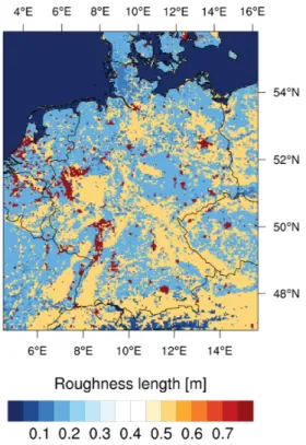
4.5.1 Roughness length . . . 66
4.5.2 The YSU PBL scheme . . . 68
4.5.3 Experimental setup . . . 70
4.5.4 Results . . . 71
5 Evaluation of an ultra large wind power ensemble 75 5.1 Experimental setup . . . 75
5.2 Case study selection . . . 76
5.3 Meteorological situation . . . 79
5.4 Results . . . 79
5.4.1 Meteorological evaluation . . . 79
5.4.2 Wind power evaluation . . . 85
5.5 Outlook: Evaluation of an ultra large solar power ensemble . . . 90
6 Summary 95
7 Conclusion and outlook 99
A Verification statistics at measurement towers 101
List of Figures
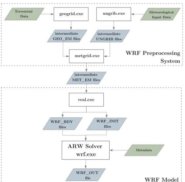
3.1 Flowchart of the WRF modeling system . . . 23 3.2 Parallel scaling behavior of the WRF model on JUQUEEN . . . 26 3.3 Necessary symmetry conditions of complex Gaussian white noise in the
SPPT and SKEB scheme . . . 28 3.4 RMSE of increments in ensemble mean of 100 m wind speed obtained
with the initialSTOCH code and modified versions . . . 31 3.5 RMSE of increments in ensemble spread of 100 m wind speed obtained
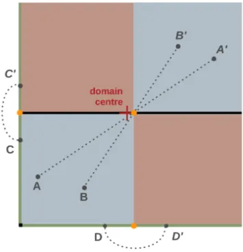
with the initialSTOCH code and modified versions . . . 31 3.6 Visualization of the MPI concept to modify the WRF modeling system
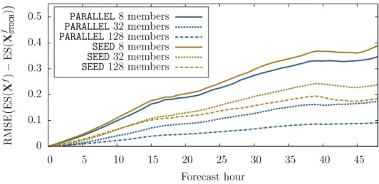
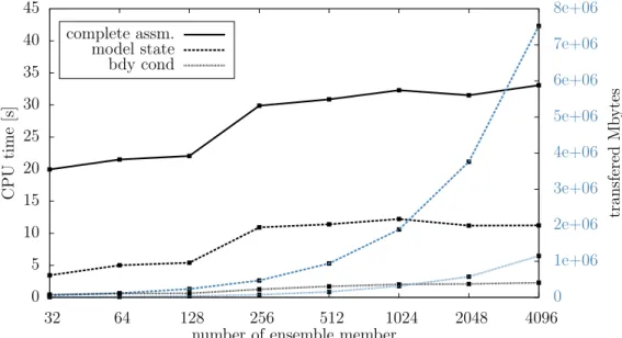
to a stand-alone ensemble control system . . . 33 3.7 CPU times and amount of transferred data for a complete particle filter
resampling step with ESIAS-met . . . 39 3.8 Flowchart of the ESIAS-met modeling system . . . 40 4.1 WRF domain configuration with its nesting procedure on a terrain
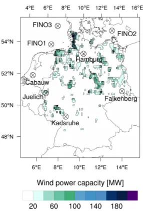
height map . . . 43 4.2 Spatial distribution of onshore wind power capacity over Germany, as
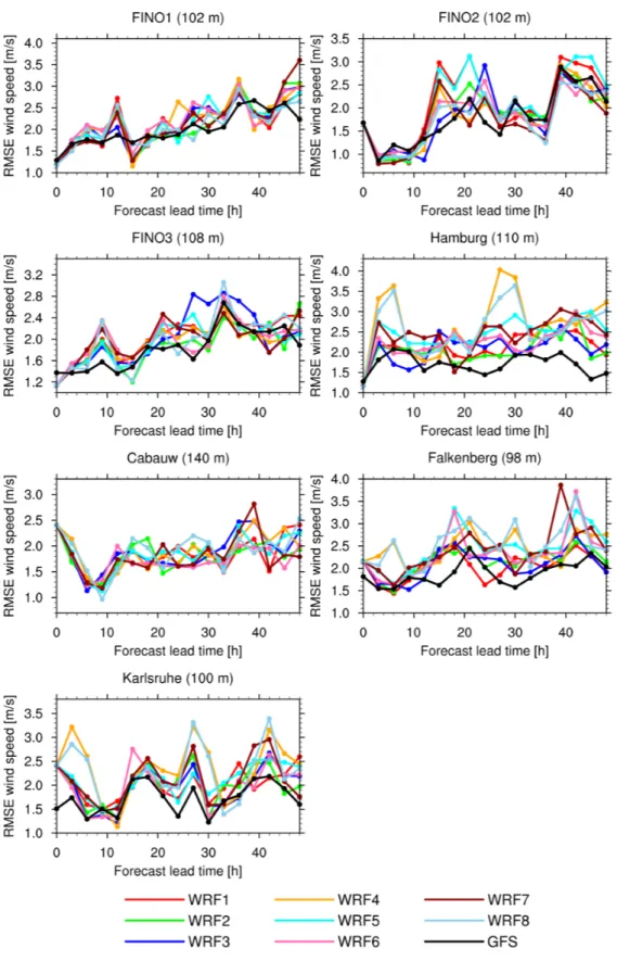
of 2014, and location of measurement towers . . . 49 4.3 RMSE of hub height wind speeds at measurement towers
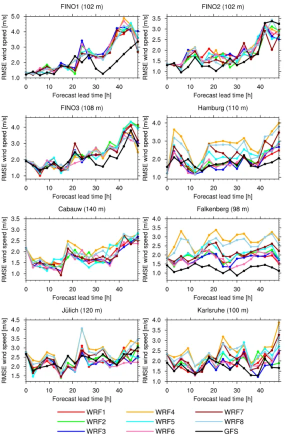
for eight different WRF model configurations, 1 – 31 August 2014 . . . 59 4.4 RMSE of hub height wind speeds at measurement towers for eight
different WRF model configurations, 1 – 30 November 2014 . . . 60 4.5 Diurnal cycle of verification statistics for the day-ahead wind power
forecast with eight different WRF configurations, 1 – 31 August 2014 . 62 4.6 Diurnal cycle of verification statistics for the day-ahead wind power
forecast with eight different WRF configurations, 1 – 30 November 2014 . . . 63 4.7 Roughness length over Germany according to the WRF model . . . . 67 4.8 Diurnal cycle of verification statistics for day-ahead wind power fore-
cast with optimized WRF configurations, 1 – 31 August 2014 . . . 72 iii
iv LIST OF FIGURES
4.9 Diurnal cycle of verification statistics for day-ahead wind power fore- cast with optimized WRF configurations, 1 – 30 November 2014 . . . 73 5.1 Instantaneous SPPT perturbation pattern . . . 77 5.2 Instantaneous SKEB perturbation patterns . . . 77 5.3 TSO day-ahead wind power forecast and real power feed-in on 9 August
2014 . . . 78 5.4 NCEP GFS analysis at 9 August 2014 . . . 80 5.5 Meteosat Second Generation SEVIRI satellite imagry, channel 9,
10.8µm . . . 80 5.6 Forecast-minus-analysis increment of mean sea level pressure at
12 UTC 9 August 2014 . . . 81 5.7 Ensemble spread of 100 m wind speed for the 1024-member ensemble . 82 5.8 Spaghetti plot of geopotential height for the 1024-member ensemble . 83 5.9 Nested quantiles of hub height wind speeds at measurement towers . . 84 5.10 Day-ahead forecast of the ultra large wind power ensemble for 9 August
2014 . . . 86 5.11 Nested quantiles of day-ahead wind power forecast for 9 August 2014 . 86 5.12 Day-ahead forecast of the ultra large wind power ensemble for 9 August
2014 (SPPT) . . . 87 5.13 Day-ahead wind power forecast of ensemble member 305 and 558 for
9 August 2014 . . . 88 5.14 Root moments of wind power distribution from n= 2 to n= 5 for 9
August 2014 . . . 89 5.15 Nested percentiles of standard deviation for bootstrapped samples of
different ensemble sizes (wind power case study) . . . 91 5.16 Nested percentiles of skewness for bootstrapped samples of different
ensemble sizes (wind power case study) . . . 91 5.17 Day-ahead forecast of the ultra large solar power ensemble for 28
November 2014 . . . 92 5.18 Root moments of solar power distribution from n= 2 to n= 5 for 28
November 2014 . . . 93 5.19 Nested percentiles of skewness for bootstrapped samples of different
ensemble sizes (solar power case study) . . . 94 A.1 Bias of hub height wind speeds at measurement towers for eight differ-
ent WRF model configurations for 1 – 31 August 2014 . . . 102 A.2 Correlation between hub height wind speeds and model data at mea-
surement towers for eight different WRF model configurations for 1 – 31 August 2014 . . . 103
LIST OF FIGURES v
A.3 Bias of hub height wind speeds at measurement towers for eight differ- ent WRF model configurations for 1 – 30 November 2014 . . . 104 A.4 Correlation between hub height wind speeds and model data at mea-
surement towers for eight different WRF model configurations for 1 – 30 November 2014 . . . 105
vi LIST OF FIGURES
List of Tables
2.1 Sources of uncertainties in NWP models . . . 9 3.1 CPU times of the WRF model on JUQUEEN with initial and improved
compiler instructions . . . 26 3.2 CPU times of the WRF model with the SKEB scheme and varying
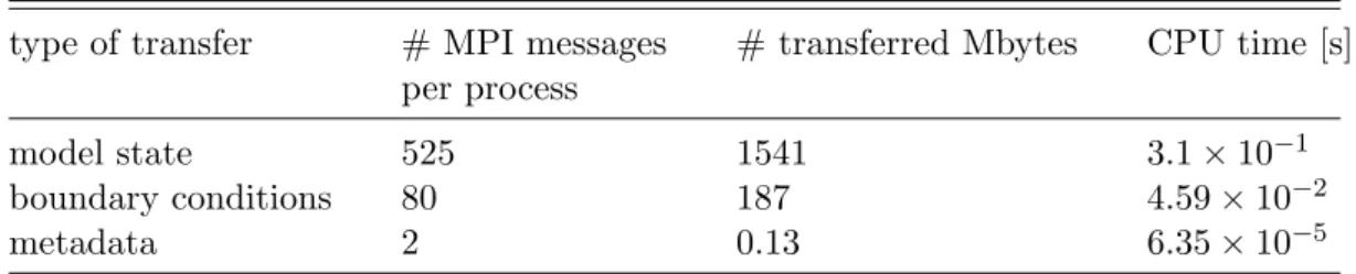
processor number for different implementations of the STOCHcode . . . 29 3.3 CPU times of ESIAS-met with increasing ensemble size . . . 36 3.4 Number of MPI messages, transferred Mbytes and CPU times associ-
ated with a resampling procedure within ESIAS-met . . . 38 4.1 Configuration of the WRF model domain . . . 43 4.2 Site characteristics of onshore measurement towers . . . 48 4.3 Summary of eight WRF configurations with different physical param-
eterizations . . . 51 4.4 Verification statistics for day-ahead forecasts with eight different WRF
configurations and GFS model fields for conventional in situ observa- tions, 1 – 31 August 2014 . . . 56 4.5 Verification statistics for day-ahead forecasts with eight different WRF
configurations and GFS model fields for conventional in situ observa- tions, 1 – 30 November 2014 . . . 57 4.6 Verification statistics for the day-ahead wind power forecast with eight
different WRF configurations, 1 – 31 August 2014 . . . 64 4.7 Verification statistics for the day-ahead wind power forecast with eight
different WRF configurations, 1 – 30 November 2014 . . . 64 4.8 Experimental setup of WRF model optimizations . . . 70 4.9 Verification statistics for the day-ahead wind power forecast with op-
timized WRF model configurations, 1 – 31 August 2014 . . . 71 4.10 Verification statistics for the day-ahead wind power forecast with op-
timized WRF model configurations, 1 – 30 November 2014 . . . 71 5.1 Stochastic model parameter for the SPPT and SKEB scheme . . . 76
vii
viii LIST OF TABLES
List of Acronyms
ARW Advanced Research WRF
BV Breeding Vector
CONUS Contiguous United States
ECMWF European Centre for Medium-Range Weather Forecasts
EM Ensemble Mean
EPS Ensemble Prediction System
ES Ensemble Spread
ET Ensemble Transformation
ESIAS Ensembles for Stochastic Integration of Atmospheric Systems
GFS Global Forecast System
GEFS Global Ensemble Forecast System IFS Integrated Forecast System
IWES (Fraunhofer)-Institut f¨ur Windenergie und Energiesystemtech- nik
LSM Land Surface Model
MPI Message Passing Interface NetCDF Network Common Data Format
NCEP National Centre for Environmental Prediction NOAA National Oceanic and Atmospheric Administration OpenMP Open Multi-Processing
PDF Probability Density Function
PBL Planetary Boundary Layer
RMSE Root Mean Square Error
SIMD Single Instruction, Multiple Data SIR Sequential Importance Resampling SIRF Sequential Importance Resampling Filter SMT Simultaneous Multithreading
SPPT Stochastically Perturbed Parameterization Tendency (scheme) ix
x LIST OF ACRONYMS
SKEB Stochastic Kinetic Energy Backscatter (scheme)
SV Singular Vector
TSO Transmission System Operator
WRF Weather Research and Forecasting (model)
Chapter 1
Introduction
A limited predictability of the atmospheric state imposes wind power as an energy source of inherent uncertainty in space and time. With the increasing amount of installed wind power capacity, accurate wind forecasts have become invaluable for the energy sector (Giebel et al., 2011; Bremen and Wessel, 2015). In meteorology, the realm of predictability is a research area of its own (Kalnay, 2003; Palmer and Hagedorn, 2006), which aims to quantify the flow-dependent uncertainties of forecasts.
Yet, predictability issues on weather dependent energy production are subdued by the technical and economical constraints of the energy system. In Germany, the infeed from renewable energy sources has priority over conventional electricity generators by governmental legislation, while transmission system operators (TSOs) have to ensure that supply matches demand to facilitate a secure electrical grid. In the day-ahead notice, balance responsible parties report expected load schedules for the following day (Hirth and Ziegenhagen, 2013). TSOs derive aggregated forecasts for the control area of Germany to anticipate regulations of power plants or negotiate supply, and accordingly, pricings are formed on the energy stock exchange. On the following day, if schedules deviate from the actual supply, balance responsible parties have the chance to adjust their portfolio on the intraday energy market (Schroedter-Homscheidt et al., 2015). Here, prices can even be negative, in case companies need to pay for undloading excess power. The TSOs take care of any remaining imbalances by activating physical control capacities to safeguard the electrical grid stability. The allocation of the associated costs, the balancing price, is distributed among the balance responsible parties. The accuracy of day-ahead wind power forecasts is therefore not only crucial for electrical grid stability, but also for an economically viable integration of wind power into the electrical grid (Hirth and Ziegenhagen, 2013).
In general, numerical weather predictions (NWPs) are the basis for wind power forecast systems for the day-ahead horizon (Focken et al., 2001; M¨ohrlen and
1
2 Introduction
Jørgensen, 2008; Vogt et al., 2016). Power curves convert model wind speed and direction at turbine hub heights to wind power, and are either provided by the manufacturer or derived for a whole region of wind farms upon historical data (Lydia et al., 2014). Forecast systems utilized by the TSOs are based on multiple NWP systems and are optimized by model output statistics to remove systematic errors.
Thereby, Germany can be treated approximately as one control area (Zolotarev and G¨okeler, 2011) and local forecast errors are in general reduced by spatial smoothing effects (Focken et al., 2002). Nevertheless, the principle forecast skill is mainly determined by the underlying NWP system (Giebel et al., 2005).
It is generally agreed that current wind power forecast systems show on average a satisfactory forecast accuracy. However, there still exist exceptional error events in the day-ahead forecast which are a major obstacle to a stable and safe grid operation. Such events are caused by an erroneous representation of the atmospheric state by all available NWP systems at that time (Dobschinski et al., 2017). Even area aggregation across multiple countries may not be sufficient to balance the forecast errors (M¨ohrlen and Jørgensen, 2017). Exceptional error events are rare by definition, corresponding to 0.05% of all times where the demand for control power exceeds the actual capacity (Consentec, 2010). According to Stark (2015), balancing prices, which are in general of the order of ±10e/MWh, may go up to
±6000e/MWh, and a trader’s one month’s profit may be ruined at the energy stock exchange (Good, 2017). Since 2012, the German Bundesnetzagentur introduced an additional penalty of 100e/MWh to the balance responsible parties, if at least 80%
of the control power capacity have to be utilized by the TSOs (Consentec, 2012).
The revenue is shared among the consumers, however, the maintenance of control power capacity is incorporated in the electricity price. Therefore, exceptional error events in the day-ahead forecast are not only critical and costly to participants of the energy sector, but also put a constant and disproportionate cost on the electricity price and are a major obstacle to the integration of wind power into the electrical grid.
Lundgren(2015) summarizes critical weather conditions which led to exceptional error events in the past. For wind power, these conditions include strong cyclogenesis, i.e. the intensity and spatiotemporal position of low pressure systems and associated frontal movements. Further, winterly stable conditions and a pronounced summerly diurnal cycle may cause severe systematic errors. For solar power, these conditions include cloud coverage after the passage of a cold front, the spatiotemporal evolution of convective systems, formation or clearing of low stratus and large-scale dust events. Exceptional error events in wind power forecasts are hence linked to meteorological events of low predictability (Steiner et al., 2017), which rest on inevitable shortcomings of todays NWP systems that all major
3
weather centres around the world face.
In this sense, a single deterministic forecast from a NWP system has a fundamentally limited usefulness. Since the pioneering work of Lorenz (1963), the atmospheric evolution is well known to be highly sensitive to its initial conditions, characterizing its dynamics as a chaotic system. Any NWP forecast must therefore be furbished with likelihood. Hence, exceptional error events can only be anticipated by a forecast of forecast skill, leading to a stochastic extension of the model’s equations. Formally, the stochastic evolution of the atmospheric state with uncertain initial conditions is described by the Liouville equation, and as a stochastic-dynamic extension by the Fokker-Planck equation. However, the only feasible approach leads to the integration of model ensembles, which approximate the probability density function (PDF) of the model state by a finite sample of different realizations of the NWP model (Epstein, 1969;Leith, 1974).
Ensemble forecasting has become a common procedure at weather centres in the last decades (Toth and Kalnay, 1997; Molteni et al., 1996; Li et al., 2008;
Denhard et al., 2016). Their undisputed success has been based on the identification of flow-dependent perturbations of initial conditions that exhibit the fastest growing modes (Toth and Kalnay, 1993; Buizza et al., 1999). Model uncertainty representation has proven to reduce the lack of dispersion among the ensemble members and thereby correcting the estimation of predictability (Palmer et al., 2009; Berner et al., 2011). Most notably, convective scale instabilities, boundary layer dynamics, cloud induced modulation of insolation, and the various mechanisms to trigger or influence these processes, must be accounted for in the parameterization of physical processes by various perturbations. Furthermore, ensemble forecasting is meanwhile also applied to mesoscale convection-permitting NWPs (Wang et al., 2008;Bouttier et al., 2012;McCabe et al., 2016;Hagelin et al., 2017). The usefulness of mesoscale ensemble modeling is based on the notion, that although higher resolution and enhanced representation of sub-grid scale processes produce more realistic forecasts of severe weather phenomena, yet it is challenged by the proper simulation of small scale processes such as convection and cloud formation (Mass et al., 2002; Eckel and Mass, 2005; Theis et al., 2005). This notion is supported by the work of (Lorenz, 1969), who showed that errors tend to grow more quickly in time with increasing resolution.
Ensemble forecasting samples the PDF of the model state, subject to all available information of uncertainty in the initial conditions and model formulation. This procedure is essentially restricted by the sample size due to limited computational resources. Operational ensembles of global circulation and convection-permitting models are all of the order of O(10) ensemble members. Examples are the Global Ensemble Forecasting System (GEFS) at the National Centre for Environmental
4 Introduction
Prediction (NCEP): 21 member; the Ensemble Prediction System (EPS) at the European Centre for Medium-Range Weather Forecasts (ECMWF): 51 members;
the ICOsahedral Nonhydrostatic ensemble at the German Weather Service (DWD):
40 members; the Met Office ensemble system (MOGREPS-UK): 20 members;
the high-resolution rapid refresh (HRRR) ensemble of the Weather Research and Forecasting (WRF) model at the National Oceanic and Atmospheric Administration (NOAA): 20 members. Numerous studies have proven, that a limited ensemble size restricts the ensemble performance (Richardson, 2001; Mullen and Buizza, 2002;
Hagelin et al., 2017), driven by the certainty, that the sampling error of the sample mean is proportional to√
N, with N the ensemble size.
Besides a restriction in the ensemble size, approximations and linearizations in NWP data assimilation techniques prohibit the capture of exceptional error events.
Despite their sophistication and acknowledged performance in NWP systems (Rabier et al., 2000; Fisher et al., 2011; Bishop and Hodyss, 2011; Wang and Lei, 2014), operational methods all rest on Gaussian assumptions. Gradient methods minimize a cost function, and in case of multimodal prior distributions, it is not clear whether this minimization converges towards a global minimum. Four-dimensional variational data assimilation (Courtier et al., 1994) adds spatiotemporal consistency.
However, an adjoint model is involved which relies on linearizations. The Ensemble Kalman Filter (Evensen, 1994) assumes normal distributions for observations as well as the model state. Although the forecast model itself is nonlinear, the Ensemble Kalman Filter forms a Gaussian posterior, characterized by the ensemble mean and associated covariances. Consequently, all operational data assimilation methods tend to prohibit the capture of exceptional error events, as the evolution of low probability tails in the prior and posterior PDF is suppressed.
Particle filters are increasingly gaining attention in the survey of a nonlinear data assimilation technique (van Leeuwen, 2009). The particle filter solves the full data assimilation problem, equivalent to Bayes’s theorem for probability densities, without any assumption on the prior and posterior model state PDF. Each ensemble member, also referred to as a particle, is related to a posterior weight according to the likelihood upon observations. Resampling reduces the variance among the ensemble members by rejection of members with low weights and duplication of members with high weights (Douc et al., 2005). Thereupon, low probability events have the potential to survive the assimilation procedure of the particle filter, though the likelihood remains small by resampling.
The application of particle filters in high-dimensional systems faces a major obstacle. The only approximation to the nonlinear solution of the data assimilation problem is in the ensemble size. Yet, ensemble sizes of NWP systems are comparably small and the particle filter in its basic form tends to degenerate. In practise,
5
a single member is assigned with all the weight and a posterior PDF becomes meaningless (Snyder et al., 2008). Upon this notion, many different variants of the particle filter have been proposed. All have in common, that they rely on improving the ensemble members’ likelihood to achieve posterior weights of similar sizes. The notion is to draw the ensemble members towards observations to form a proposal density which is subject of sampling. One might simply think of a Gaussian of a local Ensemble Kalman Filter step as proposal density, or to nudge the ensemble members towards observations (van Leeuwen, 2009). More sophisticated methods target similar weights by construction, e.g. the implicit particle filter (Chorin et al., 2010), which introduces an optimal proposal density by mapping the implicit sampling space to the original state space, or the equal-weight particle filter (van Leeuwen, 2010), which obtains equal weights by a proposal density which depends on all members at the previous time steps. The localized particle filter (Poterjoy, 2016) adopts the idea of localization used in the Ensemble Kalman Filter to formulate weights with a limited radius of influence. The class of particle smoothers weights the ensemble at the current time step upon information of the likelihood at a future time step. One can think of many variants, with the auxiliary particle filter being the most prominent (Pitt and Shephard, 1999). However, despite the sophistication involved in all the approaches listed above, the ensemble size still remains crucial for their performance.
Resampling requires inter-member communication and autonomous ensemble execution appears therefore suboptimal. Further, the variance among ensemble members should ideally be monitored frequently prior to the occurrence of filter degeneracy. Both requirements may lead to substantial computational times for ensemble sizes beyond state-of-the-art. It is not necessarily clear how a software environment for this purpose may be designed, as yet no convenient approach has been proposed in the literature.
Studies on the benefit of ultra large ensemble sizes are a rarity. The terminology of ultra large refers here to ensemble sizes beyond 1000 members. Already Buizza and Palmer(1998) point out, that an increase in ensemble size beyond 100 members is expected to have a beneficial impact on the outlier statistic, which is the key score for any prediction of exceptional error events. Miyoshi et al. (2014) realize a 10,240-member ensemble of an intermediate atmospheric model and investigate the Gaussianity of the forecast PDF. For less than 10 % of the forecast time, they find pronounced non-Gaussianity PDFs, and for less than 1 % a pronounced bimodality.
However, they conclude, a minimum of O(1000) ensemble members is needed to resolve this non-Gaussianity. It can be assumed, that these results amplify in the case of a full atmospheric model, especially in the mesoscale, as higher resolution increases nonlinearity. Therefore, non-Gaussian model PDFs will most likely be
6 Introduction
suppressed by the sampling error of operational ensemble systems, leading to insufficient representation of exceptional error events.
To summarize, the predictability of exceptional error events in wind power forecasting is likely limited by a restricted ensemble size and Gaussian data assimilation techniques in NWP modeling. Thereupon, this work increases the standard ensemble sizes in NWP modeling from the order of O(10) to O(1000) members in the frame of a demonstrator system. For this purpose, the Weather Research and Forecasting (WRF) model (Skamarock et al., 2008) is applied, a state-of-the-art mesoscale NWP model. Each ensemble member realizes a convection-permitting, high-resolution forecast over the target area of Germany. The ultra large ensemble size appears particularly favorable to apply particle filtering or smoothing techniques as a nonlinear data assimilation technique. A software environment shall be developed which realizes particle filtering computational efficient, independent of the ensemble size.
The work’s objectives may be summarized by the following questions:
• How may a software environment be designed which efficiently executes particle filtering with an ultra large ensemble size?
• What is the benefit of increasing the ensemble size of NWP models with respect to the predictability of exceptional error events in wind power forecasting?
This thesis is structured as follows: Chapter 2 formally introduces ensemble forecasting, with a particular attention to the methods utilized to generate the ultra large ensemble. Further, the basic particle filter and resampling methods are described as a basis for any software developments to follow. Chapter 3 presents a strategy to execute the particle filter in the realm of an ultra large ensemble size in a convenient and computational efficient way. A proof of concept is demonstrated on a Blue Gene system in the frame of a feasibility study.
Chapter 4 is designed to set the stage for the ultra large wind power ensemble.
The WRF model setup is described in detail and the wind power model is introduced. A further aim is to derive the best possible deterministic forecast to serve as the model setup for the ultra large ensemble. Thereby, Chapter 4 touches upon model optimization of the surface boundary conditions and planetary boundary layer parameterization. Chapter 5 presents an evaluation of the ultra large ensemble on one of the major error events in wind power forecasting of the last years. Results are evaluated against meteorological observations and the real wind power feed-in. Additionally, an analysis of a solar power case study supports the main findings. A summary of the work is given in Chapter 6.
Concluding remarks appear in Chapter 7 and directions for future work are presented.
Chapter 2
Ensemble forecasting and nonlinear data assimilation
Ensemble forecasting aims to quantify the flow-dependent uncertainty of the at- mospheric state derived by a NWP model. A finite ensemble size of different model formulations initialized from perturbed initial conditions shall represent an indistin- guishable sample of the probability density function (PDF). Ensemble-based data as- similation techniques incorporate this uncertainty information to formulate the prior likelihood of the model state. Here, the class of Sequential Importance Resampling Filters and Smoothers is of special interest, as the only approximation in their for- mulation is the ensemble size. This chapter serves the purpose to introduce both, ensemble forecasting and nonlinear ensemble-based data assimilation.
2.1 Uncertainties in Numerical Weather Predictions
Uncertainties in Numerical Weather Prediction (NWP) models are in general di- vided into two types: initial condition error and model error. This distinction has been proven to be practical, as different approaches to address uncertainty target either one of them. However, it should be stressed that initial condition and model error1are in principle inseparable, as model errors project on the analysis uncertainty and vice versa.
Formally, a numerical integration of the NWP model may be written in its sim- plest form as (Berner et al., 2015)
xf =xa+ Z T
t=0
∂[x]dyn
∂t + ∂[x]param
∂t
dt, (2.1)
1The distinction between forecast error and model error as defined inDaley(1991) is not followed here.
7
8 Ensemble forecasting and nonlinear data assimilation
wherexf =x(T) denotes the model state forecast,xa=x(0) the model state analy- sis,tthe time andT the forecast length. The contributions to the tendencies from the dynamical core [x]dyn and the parameterizations [x]param are written separately. In the context of ensemble forecasting, this states the control model andxf is denoted as the control, or unperturbed ensemble member forecast, subject to all available knowledge of initial conditions and model formulation. Initial condition error is in- herent inxa, and model error inRT
t=0
∂[x]
dyn
∂t +∂[x]∂tparam
dt.
Accordingly, an ensemble forecast is formulated as a set of model integrations given by
xfi = (xa+x0ai ) + Z T
t=0
∂[xi]dyn
∂t + ∂[xi]param(stoch)
∂t +∂[xi]stoch
∂t
dt, (2.2) where xfi denotes the model state of the ith ensemble member forecast, with i ∈ {1,· · · , N} and N the ensemble size. Each ensemble member is integrated forward in time starting from a different analysis, subject to perturbation x0ai , with xai = xa+x0ai , where the analysis xa of the control member is typically derived by an independent data assimilation system. The contribution from parameterizations are reformulated here as [xi]param(stoch), subject to a possible stochastic perturbation.
Possible contributions from additional processes that stem from model uncertainty are denoted as [xi]stoch. It is assumed that the dynamical core stays unperturbed in the ensemble formulation.
Errors in the initial conditions stem from a limited observability of the atmospheric state as well as measurement and representativity errors. This uncertainty evolves in the data assimilation process, subject to approximations and restricted knowledge of error covariances. Errors in the model formulation stem from unresolved process appearing on the sub-grid scale, lower boundary forcings and ultimately the numerical formulation of model equation. Table 2.1 summarizes sources of uncertainties and lists further examples.
2.2 Representation of initial condition error
The chaotic behavior of the atmosphere is known to be formulated in its sensitiv- ity to the initial conditions (Lorenz, 1963). Ideally, a finite ensemble size selectively samples the probability density function of the initial conditions (or analysis), such that the possible ranges of model outcomes are covered to the best possible extend.
Different selective sampling strategies differ in how they estimate the initial condition PDF and how it is sampled.
2.2 Representation of initial condition error 9
Table 2.1: Sources of uncertainties in NWP models divided in the categories of initial condition error and model error.
Error category Sources
Initial conditions Observations, e.g.
• restricted observational coverage
• measurement error
• representativity Data Assimilation, e.g.
• linearization, Gaussian errors statistic
• mapping between model state and observations state
• static or limited knowledge of flow dependent background covariance
Model Unresolved processes, e.g.
• parameterizations of physical processes
• closure assumptions
• feedback of energy from unresolved to resolved scales Lower boundary forcings, e.g.
• land surface parameter: roughness length, albedo, moisture availability, vegetation fraction
• sea surface temperature Numerical processing, e.g.
• numerical diffusion
• truncation error and precision
The first operational implementation of ensembles2 emerged in the same years at the European Centre for Medium-Range Weather Forecasts (ECMWF,Buizza et al.
(1999)) and the National Centre for Environmental Prediction (NCEP, Toth and Kalnay(1997)). Their undisputed success arose by the notion, that perturbations in the initial conditions exhibit different growth rates, favored by the underlying atmo- spheric flow. In other words, the sampling of the analysis PDF shall be confined to the subspace of the fastest growing perturbations. Different selective sample strate- gies have been proposed to identify such perturbations which are most relevant for the model dynamic.
The singular vector (SV) method (Buizza et al., 1999) samples the analysis PDF by perturbations which possess the largest linear growth rates over a fixed optimiza- tion interval. The directions of such perturbations are given by the singular vectors of the tangent linear model, which are computed by applying the tangent linear model forward and backward. In practice, this equals an iteratively solution of an eigenprob- lem given by the tangent linear model and its adjoint, with respect to a predefined
2At the same time, the Meteorological Service of Canada (MSC) implemented an 16-member ensemble based on the Perturbed Observation (PO) method (Houtekamer et al., 1996). Due to its limited success, it is not further discussed.
10 Ensemble forecasting and nonlinear data assimilation
energy norm. The SV method owes its success to a rapid error growth, which max- imizes ensemble spread and various probabilistic skill scores. Analysis perturbations x0ai are given by a linear combination of singular vectors for the norther hemisphere, southern hemisphere and the tropics, each scaled by analysis error estimates (Molteni et al., 1996). The ensembles generated in this work have been finally initialized by a different ensemble system (see the discussion of Section 4.1.2), and therefore, the SV method is not discussed in further detail.
The breeding vector (BV) method (Toth and Kalnay, 1993, 1997) has been es- tablished at NCEP and is based on the notion, that uncertainties in the analysis are dominated by short-range forecast errors. Initial random perturbations added to the analysis xa will, after a sufficient number of assimilation cycles, grow into the direction of the leading local Lyapunov vectors of the dynamical system3. If pertur- bations are rescaled at the end of each assimilation cycle, growing perturbations will amplify with respect to nongrowing perturbations. The BV method comes with no further expense and may be divided in the following steps: (i) a random perturbation is added initially to the analysis, (ii) the model is integrated forward in time from the perturbed and control analysis, (iii) the difference of both is formed and rescaled, (iv) the negative and positive (paired) of this difference define the new perturba- tions added to the control analysis. This procedure is cycled, restarting from (ii). It is stressed again, that any initial random perturbation introduced at (i) will evolve according to the local stability properties of the underlying atmospheric flow. The breed vectors evolve according to the full nonlinear model, unlike the singular vectors which are computed under the assumption of linearity. The BV method samples the analysis PDF by the breeding vectors, and the analysis perturbations can be written as
x0ai = R(λ, φ, t)xBVi , (2.3) wherexBVi denotes theith breeding vector and R defines a regional rescaling factor, withλthe latitude and φ the longitude, which modifies the perturbation amplitude according to a spatial climatological difference in the analysis error variance derived by two different perturbed data assimilation cycles (Toth and Kalnay, 1997).
This investigation makes use of initial condition perturbations constructed by the Ensemble Transform method with rescaling (ETR, (Wei et al., 2008)), which is thereupon introduced more formally. The ETR method is based on the notion, that breeding is suboptimal in that it is firstly, not consistent with the data assimilation system, as perturbations do not project on the analysis error variance and the regional
3Local Lyapunov vectors define the directions in which random perturbations will grow. Their associated Lyapunov exponents determines convergence or divergence of neighboring points in the phase space and hence, characterize the system’s stability (within the linear approximation). The BV method is a ”nonlinear generalization of the method used to construct Lyapunov vectors” (Kalnay, 2003). For a review, the reader is referred toKalnay(2003) andStrogatz (2014).
2.2 Representation of initial condition error 11
rescaling mask is constructed based on a climatology, and secondly, perturbations do not effectively cover the possible degree of freedom as they are not necessarily orthogonal, but paired. The ETR method can be understood as an extension of the BV method, which addresses both shortcomings.
In the Ensemble Transform (ET), analysis perturbations are obtained by
X0a=X0fT, (2.4)
where X0f = {x0f1, . . . ,x0fN} and X0a = {x0a1, . . . ,x0aN} are K ×N matrices with the ith column given byx0fi =x0i−xf and x0ai =xai −xa, respectively, andK the model state dimension. The ensemble mean forecast is defined as xf = N1 PN
i=1xfi. The transformation matrixT is chosen such that initial conditions in the ensemble shall be restrained explicitly by the analysis error covariance
TT(X0fTP−1a X0f)T=I. (2.5) The matrix Pa is assumed to be diagonal and contains analysis error variances, es- timated by an assimilation system. Equation (2.5) ensures, that the variance of the analysis perturbationsX0aequals that ofPa, under the assumption thatX0f reflects the real forecast variances. The transformation matrix T is obtained by solving the eigenvalue problem
XfTP−1a Xf =CΓC−1, (2.6)
where the orthogonal eigenvectors ci are listed column-wise in matrix C and the eigenvalues λi are listed in descending order in the diagonal matrix Γ, with i ∈ {1,· · · , N}. Wei et al. (2008) shows that only the first N −1 eigenvalues are non zero. Thereupon, a matrix G may be defined, which sets the Nth eigenvalue to a non zero constant, and the transformation matrixT is derived as
T=CG−1/2. (2.7)
Analysis perturbations of the ET are orthogonal under a norm defined by the inverse of analysis error variancePa, however, they are not centered, which might degrade the ensemble mean forecast. To ensure thatPN
i=1x0ai = 0 holds, a simplex transformation is applied and the final transformation matrix reads
Tp =CG−1/2CT. (2.8)
The simplex transformation preserves the analysis covariance, but a finite number of ensemble member becomes quasi-orthogonal. The ETR method has proven to outperform the simple breeding method in various probabilistic skill scores (Wei et al.
(2008)).
12 Ensemble forecasting and nonlinear data assimilation
2.3 Representation of model error
Meteorological ensembles are well known to overestimate the atmospheric pre- dictability (Buizza et al., 1999), which appears most prominently in convection- permitting ensembles of the short-range (Romine et al., 2014). Even if one may assume perfect knowledge of the analysis distribution, the resulting ensemble still exhibits underdispersiveness (Palmer et al., 2005; Wilks, 2005). The inherent uncer- tainty in model formulation cannot be neglected in general, which may limit atmo- spheric predictability to the same extend as initial condition error. This is especially true for severe weather events, e.g. explosive cyclogenesis (Mullen and Baumhefner, 1988).
Model errors are complex in their nature and far from being fully understood.
They originate mainly from processes which appear on the sub-grid scale. Different stochastic parameterizations have been proposed and proven to increase the ensemble spread, while maximizing the ensemble reliability (Berner et al., 2011; Christensen et al., 2015). Their beneficial impact has also been reported for ensemble data assim- ilation (Ha et al., 2015), as model errors affect the uncertainty introduced by initial conditions and vice versa. Multiple types of approaches exist, since model errors stem from many different sources. Most of the operational schemes are formulated as stochastic reinterpretations of deterministic parameterizations, and are somewhatad hoc, as they are based on empirical assumptions which are formulateda priori. How- ever, the merit of existing schemes goes beyond simply increasing ensemble spread, which is in general feasible to be addressed by postprocessing, but to trigger possi- ble instabilities in the underlying flow to represent the range of possible outcomes.
Surely, the final goal to be accomplished are true stochastic parameterizations which account for uncertainty where it actually appears.
Here, the description is restricted to the Stochastically Perturbed Parameteriza- tion Tendency (SPPT) scheme and the Stochastically Kinetic Energy Backscatter (SKEB) scheme, as both have been implemented in the WRF model following closely their formulation in the ECMWF EPS ensemble. SPPT represents sub-grid scale variability of parameterizations by sampling the net parameterized physics tenden- cies around their deterministic value. In contrast, SKEB accounts for spurious model dissipation by stochastically injecting energy across various spatial scales. Despite their numerous shortcomings (Shutts, 2015), both schemes have become broadly es- tablished in ensembles of global circulation models (Berner et al., 2009;Palmer et al., 2009;Charron et al., 2010;Sanchez et al., 2016) as well as mesoscale models (Berner et al., 2011; Tennant et al., 2011; Bouttier et al., 2012; Berner et al., 2015; Shutts, 2015). Their complementary has been proven in numerous studies (Romine et al., 2014; Jankov et al., 2017), as the forcing introduced by SPPT is the largest in the tropics and in the planetary boundary layer, and by SKEB in the free atmosphere
2.3 Representation of model error 13
and in case of strong cyclogenesis.
2.3.1 Stochastically Perturbed Parameterization Tendency scheme By definition, physical parameterizations are estimations of unresolved atmo- spheric processes appearing on the sub-grid and/or evolving by processes which are insufficiently understood. Even parameters within parameterizations, arising e.g.
from closure assumptions or estimations of probabilistic mean values, possess a sig- nificant uncertainty. Their feedback on the resolved flow is sometimes understood as an ensemble mean of plausible ranges consistent with the resolved-scale forcing, e.g. for cumulus parameterization (Arakawa and Schubert, 1974). This assumption is condemned to fail with the ever increasing resolution of atmospheric models, and in one way or the other, a transition to a stochastic reformulation of parameterizations is inevitable.
The Stochastically Perturbed Parameterization Tendencies (SPPT) scheme does so in a straight forward manner by introducing univariate multiplicative noise to the net parameterized physics tendencies and reformulating their contribution to the to- tal local tendency at each grid point as a sample of a probability density function, which is centered on their deterministic value. With the nomenclature introduced for (2.1), the tendency equation for the prognostic variables x∈ {u, v, q, T}, with u and v the wind vector components, q the humidity and T the temperature, may be written as
∂[x]dyn
∂t +∂[x]param
∂t , (2.9)
and a perturbed parameterization tendency is then defined as
∂[x]dyn
∂t +∂[x]param(stoch)
∂t = ∂[x]dyn
∂t + (1 +r(x, y, z, t))∂[x]param
∂t , (2.10)
whereris a pattern which imposes spatial and temporal correlation on perturbations.
Formulations of SPPT in various ensemble systems differ essentially by the choice of r. Here, it is restricted to the formulation as implemented in WRF, following Berner et al.(2015).
Perturbations are drawn from a truncated Gaussian noise process in the range r∈[−1,1], with prescribes standard deviationη. Variations in the vertical are omitted to retain conservation laws imposed by the parameterizations, yet no instabilities in the planetary boundary layer have been reported for the WRF model. For theX×Y horizontal grid, the stochastic patternr is defined in spectral space as
r(x, y, t) =
K/2
X
k=−K/2 L/2
X
l=−L/2
rk,l(t)e2πi(kx/X+ly/Y), (2.11)
14 Ensemble forecasting and nonlinear data assimilation
with Fourier modesrk,l depending on wavenumbers k, l in zonalx and meridional y direction of WRF’s rectangular grid, respectively. A first-order autoregressive process imposes temporal correlation
rk,l(t+ ∆t) = (1−α)rk,l(t) +tk,l
√αk,l(t), (2.12)
such that small perturbations are associated with a short temporal range and vice versa. This describes a Markov process, (1−α) is the autoregressive parameter with α= ∆t/τ ∈(0,1] andτ the decorrelation time. k,l is a complex Gaussian white noise process with zero mean and covariance h(s)k,l∗(t)m,ni =σ2δk,mδl,nδs,t, with σ2 set to one. The variance spectrum of the first-order autoregressive process is determined by the amplitudes tk,l, which are defined such that they yield an autocorrelation according to a Gaussian on a plane:
tk,l =F0exp(−4πκρ2k,l), (2.13) with ρ = p
k2/X2+l2/Y2 the radial wavenumber and κ the spatial correlation length, as derived byWeaver and Courtier(2001). F0 denotes a normalization factor that depends linearly on the spectral varianceη2k,l:
F0= ηk,l(2α−α2) 2P
k
P
lexp(−8πκρ2k,l)
!
. (2.14)
The stochastic pattern’s quantities determine directly the forcing of the scheme, with the tuning parameters of standard deviationη as well as temporal and spatial corre- lationτ and κ, respectively. The default values in the WRF model are η= 0.5, with cuttoff tails above 2.0, τ = 21600 s and κ= 150 km.
Instead of a univariate formulation, one may think of perturbing each physics ten- dency independently, which was the initial ansatz proposed byBuizza et al.(1999) in the ECMWF EPS ensemble. However, multivariate perturbations are less consistent with the model physics, decrease the skill of tail distribution statistics and generate gravity waves (Palmer et al., 2009). The system tends to be pushed from its preferred attractor too often, which may exceed the range of model uncertainty.
The forcing imposed by SPPT is flow-dependent, as the perturbation magnitude scales with the accumulated tendencies. However, the probability distribution of certain parameterizations varies strongly depending on the geographical location or height. Further, uncertainties evolving in the vertical, e.g. the shape of a momentum profile in the planetary boundary layer, can not be represented.
2.3 Representation of model error 15
2.3.2 Stochastic Kinetic Energy Backscatter scheme
The Stochastic Kinetic Energy Backscatter (SKEB) scheme was originally devel- oped in the context of large-eddy simulations (Mason and Thomson, 1992) to account for unresolved energy transfer from the sub-grid scales to the resolved scales, known as an inverse energy cascade. Parts of the dissipated energy are reinjected stochas- tically as kinetic energy to mimic an energy spectra derived by the counterpart of a direct numerical simulation (Frederiksen and Davies, 2004). This idea was exported to NWP ensembles (Shutts, 2005; Berner et al., 2009), motivated by the excessive energy dissipation over various scales (Nastrom and Gage, 1985;Palmer et al., 2009).
Net energy sinks arise from parameterizations as well as the dynamical core, in parti- cular from unbalanced motions of orographic wave drag, convection and gravity waves as well as numerical dissipation. Hence, in the context of NWP models, the SKEB scheme is not confined to the vicinity of the truncation scale, but energy is even injected upscale to the subsynoptic and synoptic scale. Coarse-graining experiments support this assumption by identifying energy sinks across the entire wavenumber spectrum (Palmer et al., 2009; Shutts, 2013). Their high-resolution counterparts are used to tune the SKEB in a way to correct the energy spectrum accordingly, yet in a heuristic fashion.
The SKEB scheme introduces additive noise to the tendency equation (2.1), such
that ∂[x]dyn
∂t +∂[x]param
∂t (2.15)
may be rewritten as
∂[x]dyn
∂t +∂[x]param
∂t +∂[x]SKEB
∂t . (2.16)
Formulations of SKEB in various ensemble systems differ by the choice of prognostic variables subject to perturbation, i.e. [x]SKEB ⊆ {u, v, T}, the dissipative sources which are associated with such perturbations and the stochastic patternr. Here, it is yet again restricted to the formulation as in the WRF model, followingBerner et al.
(2011).
A streamfunction tendency forcing ψ0(x, y, t) := ∂ψ(x, y, t)/∂t and a potential temperature tendency forcing θ0(x, y, t) := ∂θ(x, y, t)/∂t are introduced to inject a domain averaged perturbation kinetic energy Ekin0 = ∆Ekin/∆t and perturbation potential energyEpot0 = ∆Epot/∆tat each time step ∆t. The associated forcings are defined in two-dimensional spectral space:
ψ0(x, y, t) =
K/2
X
k=−K/2 L/2
X
l=−L/2
ψk,l0 (t)e2πi(kx/X+ly/Y), (2.17)
16 Ensemble forecasting and nonlinear data assimilation
θ0(x, y, t) =
K/2
X
k=−K/2 L/2
X
l=−L/2
θ0k,l(t)e2πi(kx/X+ly/Y), (2.18) with the nomenclature of the Fourier expansion already introduced in the previous section. Perturbations of the wind vector are confined to the rotational part to pre- serve the dynamical balance between pressure and wind, withu0(x, y, t) =−∂ψ0(x,y,t)∂y and v0(x, y, t) = ∂ψ0(x,y,t)∂x the zonal and meridional wind tendency forcings, respec- tively.
Finite temporal correlations are imposed by evolving each spectral coefficient ac- cording to a first-order autoregressive process:
ψ0k,l(t+ ∆t) = (1−αψ)ψk,l0 (t) +gk,l√
αψk,l(t), (2.19) θk,l0 (t+ ∆t) = (1−αθ)θ0k,l(t) +hk,l√
αθk,l(t). (2.20) This process has already been described in-depth in the previous section by (2.12).
Here,αψ/θ = ∆t/τψ/θ ∈(0,1] again denotes the autoregressive parameter, withτψ/θ the decorrelation time. In the WRF model, temporal and spatial constant dissipation rates are assumed and hence, quantities of the first-order autoregressive process will directly transfer to the effective perturbations. This appears as a somewhat drastic simplification. However, Berner et al. (2011) shows that results are quite similar compared to a flow-dependent dissipation rate, as estimations of the true dissipation rate remain a challenge. One aims to prescribe the injected energies with a given power spectrum, yielding noise amplitudes of the form
gk,l =bρβk,l, (2.21)
hk,l=f ργk,l. (2.22)
The amount of backscattered dissipated energy determines the amplitudesband fof the forcings. For the streamfunction, an energy backscatter rate Bψ injects a total kinetic energy ∆Ekin per unit mass into the full flow during a numerical time step
∆t:
Bψ = ∆Ekin
∆t = 2π2
∆t
K/2
X
k=−K/2 L/2
X
l=−L/2
ρ2k,lh|ψk,l(t+ ∆t)|2− |ψk,l(t)|2i (2.23)
= 2π2σ2ψ∆t αψ
K/2
X
k=−K/2 L/2
X
l=−L/2
ρ2β+2k,l b2. (2.24)
2.3 Representation of model error 17
Solving forb yields:
b= Bψαψ 2πσ2ψΓψ∆t
!12
, with Γψ =
K/2
X
k=−K/2 L/2
X
l=−L/2
ρ2β+2k,l . (2.25)
This implies, that a streamfunction forcing with power lawρβk,l will result in a kinetic energy spectrum with power law ρ2β+2k,l (in radial wavenumber). Advancing in the same manner for the potential temperature, an energy backscatter rate Bθ injects during a numerical time step ∆t a total potential energy ∆Epot per unit mass into the full flow:
Bθ = ∆Epot
∆t = cp
2θ0∆tθ2 = cp θ0∆t
K/2
X
k=−K/2 L/2
X
l=−L/2
h|θk,l(t+ ∆t)|2− |θk,l(t)|2i (2.26)
= cpσθ2∆t θ0αθ
K/2
X
k=−K/2 L/2
X
l=−L/2
ρ2γk,lf2, (2.27)
with θ0 = 300 K a reference potential temperature used in the WRF model and cp= 1004 J/K the specific heat capacity. Solving forf yields
f =
Bθαθθ0
cpσ2θΓθ∆t 12
, with Γθ =
K/2
X
k=−K/2 L/2
X
l=−L/2
ρ2γk,l. (2.28)
This implies, that a potential temperature forcing with power lawργk,l will result in a kinetic energy spectrum with power lawρ2γk,l (in radial wavenumber). The derivation of (2.24) is given in the appendix ofBerner et al.(2009) (in spherical coordinates for a global circulation model), and (2.27) is derived analogously.
In the WRF model, the SKEB scheme is fully controlled by the tuning parame- ters β, γ, σψ2, σθ2, τψ, τθ, Bψ, Bθ. Default values are β =γ =−1.83, which results in a perturbation kinetic energy spectrum of−5/3 and in a perturbation potential energy spectrum of−10/3. The noise variance is set toσψ2 = (1/12)αψ,σ2θ = (1/12)αθ and decorrelation times areτψ =τθ = 10800s. The backscattered energy rates are chosen asBψ = 10−5m2/s3 and Bθ = 10−6m2/s3. For comparison, Berner et al. (2009) re- ports an annual global mean dissipation rate in the ECMWF model of 1.99 W/m2 for deep convection. With an air density of 1 kg/m3and an air column of 1 km height, this yields 1.99×10⁻³m2/s3 per unit mass. With the remaining sources approximately of the same order, and assuming 1/10 of the dissipated energy being backscattered (according to Palmer et al. (2009)), a value of 10−3m2/s3 may be estimated. The choice of backscatter rates in the WRF model is therefore rather conservative.
Current implementations of the SKEB schemes in operational ensemble systems
18 Ensemble forecasting and nonlinear data assimilation
do not come without criticism. Thuburn et al. (2013) and Shutts (2013) conclude, that at least parts of the energy sinks are likely to be of systematic nature and should rather be fixed in a deterministic manner. Further, with increasing model resolu- tion, perturbations across the whole wavenumber range used by SKEB scheme will most likely not be justifiable any more. However, as such issues remain unresolved, the SKEB scheme states an attractive approach to account for the excessive energy dissipation problem by a probabilistic approach, while, at the same time, increasing ensemble spread and improving probabilistic skill scores.
2.4 The Sequential Importance Resampling Filter
The survey of fully nonlinear data assimilation in atmospheric science has drawn large attention to Sequential Monte Carlo techniques, or simply the particle filter.
Particle filters belong to the class of recursive Bayesian estimators and solve the full data assimilation problem, with the only approximation being the limited ensemble size. For a comprehensive review, the reader is referred tovan Leeuwen (2009).
The particle filter relates a posterior weights to ensemble members, which estimate the likelihood of each model state given the observations. The prior density of the model state x may be formulated as the sum of δ-functions, centered around each ensemble member model state:
p(x) = 1 N
N
X
i=1
δ(x−xi), (2.29)
withN the ensemble size. By applying Bayes’ theorem, we find that the a posteriori density of the model state, given observationsy, reads
p(x|y) = p(y|x)p(x)
p(y) . (2.30)
Using the particle filter expression for the prior density, it follows p(x|y) =
N
X
i=1
wiδ(x−xi), (2.31)
where the weightswi are given by
wi = p(y|xi) PN
j=1p(y|xj). (2.32)
This formulation is known as Sequential Importance Sampling (SIS), or simply the basic particle filter. However, especially for high dimensional systems like the atmo- sphere, the ensemble size is very much limited and the basic particle filter tends to