Variational and perturbative extensions of continuous unitary transformations for low-dimensional spin systems

(1)

Variational and Perturbative Extensions of Continuous Unitary Transformations for Low-Dimensional Spin

Systems

Dissertation

zur Erlangung des Grades eines Doktors der Naturwissenschaften

der Fakult¨at Physik

der Technischen Universit¨at Dortmund

vorgelegt von

Nils Alexander Drescher

aus Dortmund

21. November 2014

(2)

Dissertation in der Fakult¨at Physik Technische Universit¨at Dortmund

Erster Gutachter: Prof. Dr. G¨otz S. Uhrig

Zweiter Gutachter: Dr. Kai P. Schmidt

Vorsitzender der Prüfungskommission: Prof. Dr. Dieter Suter Vertreterin der wissenschaftlichen Mitarbeiter: Dr. Bärbel Siegmann Tag der mündlichen Prüfung: 19.12.2014

(3)

3

Meinen Eltern Vera und Bernhard

Give me six hours to chop down a tree and I will spend the first four sharpening the ax.

— Unknown. Often attributed to Abraham Lincoln.

[Schwartz(2010)]

(4)

(5)

Chapter 1 Motivation and overview

Superconductivity is one of the most impressing quantum phenomena that can be observed macroscopically. Since its discovery by Onnes [Onnes(1911),Onnes(1913)], the exotic properties of the superconducting phase have triggered numerous theoretical and experi- mental studies, and as well as extensive research for industrial applications [Bray(2008), Bray(2009)].

Apparently, the ability of superconducting materials below their transition tempera- tureTcto carry high current densities without any losses due to electrical DC resistance is attractive in numerous technological applications. First of all, we mention the generation and indefinite maintenance of strong magnetic fields used in research facilities, particle accelerators like the Large Hadron Collider (LHC), and for compact and lightweight elec- tric motors and generators. So far, the biggest commercial success has been achieved by superconducting solenoids forMagnetic Resonance Imaging (MRI)devices, which provide an exceptionally high resolution for medical diagnostics without the ohmic losses and heat production of conventional copper solenoids.

An obvious application of superconductivity are superconducting wires for connecting of electrical power grids. However, superconductors are also suitable for the construction of more sophisticated power grid components, e. g. fault current limiters or superconducting magnetic energy storage. Moreover, superconductors can be used in an increasing number of electronic devices, with high quality microwave filters in cell phone base stations being the most successful commercial application [Smith & Jain(1999),Willemsen(2001)].

The exploitation of the Josephson effect in superconducting quantum interference devices (SQUIDs) allows for the measurement of magnetic fields with the accuracy of flux quanta. Eventually, the direct manipulation of magnetic flux quanta in superconducting quantum circuits is a promising candidate for the implementation of scalable quantum computers [Barends et al.(2014)].

Microscopically, the superconducting phase can be understood as condensate of two- electron bound states (Cooper pairs). For conventional superconductivity, as it has been found in pure metals or alloys like NbTi, the attractive interaction between electrons is mediated by electron-phonon coupling [Bardeenet al.(1957b),Bardeenet al.(1957a)]. The need to operate well below the transition temperature of the superconductor diminishes the technical and economical benefits of superconducting devices, since the low transition temperatures of conventional superconductors require expensive cooling by liquid helium.

For this reason, much interest has been paid to the discovery of unconventional superconductors [Bednorz & M¨uller(1986)], where the conventional, phonon-mediated mechanism can be ruled out due to the missing isotope effect [Hoen et al.(1989)]. While

(10)

different classes of unconventional superconductors have been found over the years, the pairing mechanism in this materials remains one of the most puzzling open questions in condensed matter physics. Of particular interest are cuprate superconductors, some of which remain superconducting above the boiling point of liquid nitrogen [Wuet al.(1987)]

and even up to 138 K [Dai et al.(1995)], leading to the name high-temperature superconductor (HTSC). While their high transition temperature makes them more attractive than conventional superconductors for industrial applications, the manufacturing process is more challenging.

The understanding of the pairing mechanism in HTSCs is of great interest for funda- mental research. At the same time, it has as a strong technological motivation, as it might lead to novel superconducting materials with even higher transition temperatures and im- proved mechanical properties, allowing for the widespread application of superconducting technologies.

Chemically, the cuprate superconductors consist of low-dimensional structures (chains, ladders, plains) of copper and oxygen, embedded in a matrix of various other elements.

While the host materials like La2CuO4are believed to be Mott insulators [Manousakis(1991)], doping with electrons or holes leads to normal conductance by charge carriers and, at a critical concentration, superconductivity arises. Interestingly, the materials enter the superconducting state close to the breakdown of long-range anti-ferromagnetic (AFM) order, where a quantum phase transition (QPT) to a magnetically disordered ground state happens. This suggest that the attractive interaction between charge carriers in cuprate HTSCs is mediated by magnetic fluctuations, and particular interest has been paid on the magnetic properties of the ground state and its excitations.

Because cuprate superconductors have a complex chemical and geometrical structure, complex interactions and strong electronic correlations to consider, a direct description taking all microscopic details into account seems to be desperate. In order to provide an understanding of the mechanisms that are essential for the magnetic properties and, finally, their role in the mechanism of superconductivity, a stepwise reduction of complexity is necessary. In the cuprates, the half-occupied orbitals of the Cu²⁺ ions is most important for the electronic and magnetic properties. They interact via superexchange mediated by the oxygen atoms. This system can be simplified as a Hubbard model, where each lattice site represents one orbital of a copper atom that can hold up to two electrons. In the minimal realization, only Coulomb repulsionU on the same site and a nearest-neighbour hopping t are considered as interactions. For the undoped case, i. e., for one electron per lattice site and in the limit of large U t, the system becomes a Mott insulator, where each electron is confined to a specific site and electron hopping is inhibited by the high energy of doubly occupied states. For studying the low-energy physics of the system, it is sufficient to concentrate on the spin degree of freedom of the localized electrons.

This leads us to the Heisenberg model, which describes the system in terms of effective spin-spin interactions that are a consequence of the high-energy physics in the underlying Hubbard model.

At each of these steps, processes on a large energy scale determine the properties on a lower energy scale in an intricate way. This gives rise to a large variety of effective interaction processes that appear in the effective low-energy model. Depending on which effective couplings are identified as important and which can be neglected in different parameter regimes of the macroscopic model, it can be necessary to construct different effective models in order to understand the macroscopic model in all aspects. Conversely, new insights can be gained when the couplings of the effective model are treated as free

(11)

11 parameters and the full phase diagram is explored, giving rise to novel kinds of order, exotic phases and their excitations.

Continuous unitary transformations (CUT) are a powerful framework to derive such effective low-energy models in a systematic and controlled fashion. By selection of an ap- propriate generator scheme, they offer a large degree of control over the general structure of the derived effective model. Even more, they can be used to understand the physical properties of the system in terms of conserved quasi-particles for the elementary excitations and to describe multi-particle continua and bound states, as well as response functions. The effective Hamiltonian can be diagonalized directly by the continuous unitary transformation (CUT), or used as starting point for the investigation by other methods.

In this thesis, we derive several methodological improvements of the CUT method, including perturbative and variational aspects, and apply it to low-dimensional spin systems. The thesis is structured as follows:

In chapter two, we give an introduction to the self-similar CUT (sCUT) method that serves as a starting point for the studies in the subsequent chapters and explain the computational implementation used in this thesis.

In chapter three, we develop two novel CUT-based techniques to study many-particle systems: The enhanced perturbative CUT (epCUT) method, which allows for high-order perturbative expansions for effective models beyond the limitations the existing perturbative CUT (pCUT) approach, and the directly evaluated epCUT (deepCUT) method, which allows us to obtain non-perturbative effective Hamiltonians efficiently and with a significantly larger robustness compared to sCUT. We illustrate these methods by a perturbed harmonic oscillator as pedagogic example.

In chapter four, we investigate the properties of CUTs in second quantization for systems with overlapping quasi-particle sub-spaces. These systems are a particular chal- lenge for the CUT method, because the particle-sorting generator schemes used to decouple the low-energy spectrum can fail in the case of strong overlap or yield a misleading quasi-particle picture. We investigate this in detail for a system of two coupled harmonic oscillators using deepCUT. Then, we develop a family of three novel variational generator schemes that do not suffer from the problems of the conventional particle-sorting generators. They lead to a meaningful quasi-particle interpretation even in the case of strong overlap.

In chapter five, we study the QPT in the dimerized, two-dimensional S=¹/²Heisenberg model by means of sCUT with a variational starting point. For the first time, we are able to describe a phase with a spontaneously broken continuous symmetry by means of CUT and to derive an effective model that describes both gapped triplons and gapless magnons as quasi-particles in a uniform operator representation. After this, we generalize the concept of the variational starting point and show how an optimal starting point can be obtained independent of the particularities of the model.

In chapter six, we investigate the S=1 Heisenberg chain using the deepCUT method and derive an effective model in terms of triplon quasi-particles. To this end, we use a mapping to a ladder-like S=¹/²Heisenberg system introducing a variational parameter. We analyze the low-energy spectrum and calculate energy- and momentum-resolved response functions. In particular, we are interested in the spontaneous quasi-particle decay of one triplon into two triplons. We find that, due to the strongly overlapping quasi-particle sub-spaces, the use of the variational generators is mandatory.

Finally, we summarize our findings in both English and German language.

(12)

(13)

Chapter 2 Self-similar continuous unitary transformations (sCUT)

2.6.3 Parallelization . . . 37 At first glance, condensed matter physics might appear asterra cognita: Schr¨odinger’s equation, the theory of everything at low energy scales, and the basic ingredients, electrons and nuclei, are known since the early 20^th century; the Hamiltonian of any compound can be written down exactly [Czycholl(2000)].

De facto, the complex interactions between these comparatively simple building blocks in various geometries have proven to be a cornucopia of innumerable interesting and diversified physical phenomena. The challenges in understanding these phenomena go well beyond a mere quantitative reproduction; a significant reduction of complexity by suitable representations, smart approximations and powerful effective theories is essential.

In the best case, even rough approximations can provide an understanding for the essential ingredients of complex physical phenomena. Prominent examples comprise the concepts of quasi-particles and Fermi liquid theory [Landau(1957)]. They allow for the description

(14)

of a complex, strongly-interacting, highly-correlated many-fermion-system in terms of the well-known, interaction-free Fermi gas, modified by just a few material-specific parameters that can be determined experimentally.

In the attempt to map a physical system to a renormalized Hamiltonian, where the phenomena of interest are better accessible, unitary transformations turned out to be a very versatile and powerful tool. They bear the advantage to retain the spectrum of eigenvalues when mapping a Hamiltonian to an effective model. In this manner, they allow us to decouple different degrees of freedom, e. g., different types of quasi-particles, or to map a many-particle problem to a few-particle problem of conserved quasi-particles.

In this way, the high-energy processes can be integrated out and an effective model for the low-energy physics is obtained. Eventually, the effective model can be studied by standard techniques or the degrees of freedom on the low-energy scale can be decoupled and studied individually.

Depending on the realization, different limitations appear: For a numerical, exact diagonalization to be feasible, the Hilbert space has to be kept finite, implying a finite lattice size. Some one-step transformations such as the Bogoliubov transformation [Bo- goliubov(1958a),Bogoliubov(1958b)] can be applied completely on an analytical level, but they decouple any but the most simple Hamiltonians to a limited degree only. Other unitary transformations such as the Fr¨ohlich transformation [Fr¨ohlich(1952)] require ad- ditional approximations. Another technique that relies on a multi-step transformation is the projector-based renormalization method [Beckeret al.(2002)].

In this thesis, we focus on an approach that can be understood as an infinite number of infinitesimal unitary transformations, leading to a continuous unitary transformation (CUT), that maps the Hamiltonian to an effective model. The structure of the effective model is controlled by the generator scheme.

In this chapter, we introduce the CUT with a focus on its self-similar version. We start with a discussion of CUT and the flow equation in general. In the second section, we present the various generator schemes used to derive effective Hamiltonians of different shapes. Then, we introduce a formulation of the flow equations using second quantization.

Based on this, we explain the truncation scheme characteristic for self-similar CUTs in section2.4. In the subsequent section, we describe a formalism to exploit the symmetries of the Hamiltonian in second quantization. Finally, we illustrate the key concepts of the computational implementation used in this thesis with emphasis on parallelization.

2.1 Continuous unitary transformations (CUT)

Finding a suitable transformation to map the initial Hamiltonian Hinit to an effective HamiltonianHeff of a specific shape is a sophisticated task. For a one-step transformation, it requires to anticipate the action of a possibly very complex transformation as a whole, while minimizing deviations from the desired structure of the effective Hamiltonian. The CUT method found independently by Wegner [Wegner(1994)] and G lazek and Wilson [G lazek & Wilson(1993),G lazek & Wilson(1994)] circumvents these problems using an infinite number of infinitesimal transformations, each of them bringing the Hamiltonian closer to the desired shape. Mathematically, this translates into the parametrization of the transformation

H(`) :=U(`)HU^†(`) (2.1)

(15)

2.1 Continuous unitary transformations (CUT) 15

by a continuous flow parameter ` with the initial condition

U(0) =1 ⇒ H(0) =Hinitial (2.2)

and Heff := H(∞). At each value of `, the momentary infinitesimal transformation can be understood in terms of the antihermitian generator

η(`) = ∂U(`)

∂` U^†(`) = −η^†(`) (2.3)

of U(`). By this definition, the flow of the Hamiltonian (2.1) can be described by a differential equation, denoted as flow equation

∂`H = [η(`), H(`)]. (2.4)

In this notation, the control of the direction of the flow has been shifted from U(`) to the generator η(`). The main advantage of this formulation is that the generator can be chosen as a function

η(`) = ηb[H(`)] (2.5)

of the flowing Hamiltonian itself, defined by a superoperator ηb that we call generator scheme henceforth. Therefore, it is not necessary to store the full, possibly very complex transformation U(`). Due to the feedback of the Hamiltonian on the generator, the flow equation (2.4) is non-linear. As a consequence, a suitable generator scheme can steer the generator asymptotically towards attractive fixed points of the flow equation where the Hamiltonian has the desired simpler structure.

The variety of possible generator schemes allows for a large degree of control over the shape of the effective Hamiltonian. We give an overview of the various possibilities in the next section.

For the calculation of experimentally observable quantities such as static correlations or response functions, two aspects of CUT matter: If the Hamiltonian is transformed into the renormalized basis, its structure can be chosen in a way that the determination of the ground state and excited states is easier or even trivial. However, the associated operator O has to be known in the same basis. This is achieved by the transformation of observables

∂_`O= [η(`),O(`)]. (2.6)

This has been used for the first time by Kehrein and Mielke [Kehrein & Mielke(1998), Kehrein(1999)] in their studies of dissipative quantum systems. Since the generatorη(`) has to be determined by the flowing Hamiltonian, it is preferable to carry out the integration of both equations (2.4) and (2.6) simultaneously.

While the global structure of the Hamiltonian may become simpler in the sense that different degrees of freedom are decoupled, new interaction processes arise in the flowing Hamiltonian due to the commutator in Eq. (2.4). They have to be considered as arguments of the commutator again. In any, but the most simple situations, the ensuing proliferation of more and more interaction processes leads to an infinite number of terms and the differential equations are not closed. Different strategies have been suggested to handle this problem leading to different realizations of CUTs:

(16)

Restriction to finite systems: If the system is restricted to a finite size, i. e., the Hamiltonian is a matrix of finite dimension, the flow equation can always be closed.

Inevitably, this places a severe limitation on the application to systems in the thermodynamic limits.

Perturbative CUT (pCUT): The idea of a perturbative expansion is continued sys- tematically in the pCUT method by Knetter and Uhrig [Uhrig & Normand(1998),Knetter

& Uhrig(2000),Knetteret al.(2003a)], which allows us to derive a perturbative expansion for the effective Hamiltonian up to very high orders. Under the requirements of pCUT, the perturbative flow equations can be integrated analytically and the remaining task consists in the calculation of matrix elements of the effective Hamiltonian. We will give a short overview of this method in section 3.1.

Self-similar CUT (sCUT): This version of CUT is the focus of this chapter. The Hamiltonian is approximated by a large but finite number of interaction processes in second quantization. The systematics which processes are considered is defined in the truncation scheme, cf. Sect. 2.4, based on a small parameter [Mielke(1997b),Mielke(1997a), Kehrein(2006)] or with respect to the range of the underlying process in real-space [Reis- chl et al.(2004),Fischer et al.(2010),Duffe(2010)]. For these processes, the flow equation is integrated numerically, giving rise to a non-perturbative, renormalized Hamiltonian.

Graph-theory based CUT (gCUT): In the gCUT method [Yang & Schmidt(2011)]

developed recently, the action of the Hamiltonian is decomposed into the action on finite graphs of various complexity. On each graph, the flow equation for the Hamiltonian can be solved numerically on the matrix level. At the end, the irreducible contributions of each graph are combined to obtain a non-perturbative effective Hamiltonian valid in the thermodynamic limit. This method can be seen as an extension of the exact linked-cluster expansion [Irving & Hamer(1984)] for ground-state properties. The accuracy is controlled by the maximal size of the graphs, similar to the range of processes in a sCUT with real-space truncation.

Enhanced perturbative CUT (epCUT): The epCUT method combines elements of both pCUT, i. e., the perturbative expansion of Hamiltonian and flow equation, and sCUT, i. e., the representation of the Hamiltonian in second quantization and the explicit numerical integration of the resulting differential equation system (DES) for its coefficients. By this combination, it is possible to overcome the limitations of pCUT and obtain effective Hamiltonians for a larger class of models. In addition, the special truncation of the flow equations associated with epCUT gives rise to a non-perturbative twin, the directly evaluated epCUT (deepCUT) method.

The epCUT and the deepCUT have been developed by Holger Krull [Krull(2011),Krull et al.(2012)], G¨otz Uhrig and myself; my contribution is expounded in chapter 3 of this thesis.

Due to their high flexibility, CUT-based methods have been applied to a large range of models. For an overview of the different applications, we recommend references [Kehrein(2006), Wegner(2006)] and [Krull et al.(2012)].

(17)

2.2 Generator schemes 17

2.2 Generator schemes

The choice of the generator scheme implies a large degree of control over the mapping of the initial Hamiltonian to the effective model in the limit of infinite `. A qualitative understanding of the flow induced by a generator scheme is provided by the fixed points of the flow.

If the flowing Hamiltonian converges in the limit of infinite`, the effective Hamiltonian has to commute with the generator

[η(`), H(`)]^`−→^→∞ 0 (2.7)

and the flow equation approaches a fixed point. Since the generator is determined from the Hamiltonian itself, the generator scheme puts a necessary condition on the effective Hamiltonian’s structure, e. g. diagonality or block-diagonality.

In a second step, the asymptotics of the flowing Hamiltonian in the vicinity of the fixed points can be studied. The flowing Hamiltonian can converge only to attractive fixed points, unless the initial Hamiltonian corresponds to a stationary point already¹.

However, the existence of attractive fixed points alone does not guarantee that the flowing Hamiltonian converges. The set of Hamiltonians for which the generator scheme converges is a third criterion that can be used to classify different generator schemes.

2.2.1 Wegner’s generator scheme

At first, we consider the original generator scheme introduced by Wegner [Wegner(1994)].

For each value of the flow parameter, the Hamiltonian H(`) =Hd(`) +Hnd(`) is decomposed into a diagonal part Hd(`) and an off-diagonal part Hnd(`) that shall vanish for infinite `.

Taken literally, this means to include any matrix element between different states in Hnd. However, we are completely free to include only a part of these matrix elements in Hnd; the rest is assigned to Hd(`) and converges to a finite value for ` → ∞. For this reason, the term “diagonal” is often used sloppily in the context of generator schemes and denotes the parts of the Hamiltonian to be kept. For a many-particle problem for instance, it is meaningful to decouple subspaces of different quasi-particle number leading to a block-diagonal effective Hamiltonian [Wegner(1994)].

With this decomposition, Wegner’s generator is defined as

ηW(`) =ηbW[H(`)] = [H(`), Hnd(`)] = [Hd(`), Hnd(`)]. (2.8a) On the matrix level, the generator can be written as

ηW,ij(`) = (hii(`)−hjj(`))hij(`). (2.8b) The generator depends bilinear on the Hamiltonian’s coefficients, which yields a trilinear flow equation. Because the squared Frobenius norm of the diagonal part

||Hd(`)||² =X

i

|hii(`)|² = 2X

ij

(hii(`)−hjj(`))²hij(`)hji(`) (2.9)

1If the Hamiltonian has a special symmetry, a third case is possible in which the Hamiltonian converges to a saddle point protected by symmetry.

(18)

is increasing monotonically and bounded from above, the flowing Hamiltonian has to converge always to a fixed point, where all off-diagonal elements hij vanish or connect degenerate states with hii = hjj. The original proof for finite matrices [Wegner(1994)]

has been extended to infinite systems [Dusuel & Uhrig(2004)] and self-similar truncation [Moussa(2010)], the latter one including a derivation of the generator scheme based on a variational argument.

2.2.2 Mielke’s generator scheme

In 1998, Mielke proposed a different generator [Mielke(1998)] defined on the matrix level that depends explicitly on the row and column indices

ηM,ij(`) = sign(i−j)hij(`). (2.10) In contrast to Wegner’s generator, it vanishes only if all matrix elements between different states are zero, even in presence of degeneracies.

The flow equations for the matrix elements of the Hamiltonian read

∂`hij(`) =−sign(i−j) (hii(`)−hjj(`))hij(`)

+ X

k6=i,j

(sign(i−k) + sign(j−k))hik(`)hkj(`). (2.11) In the vicinity of fixed points of the flow, i. e., diagonal Hamiltonians, the derivative is dominated by the leading term linear in the off-diagonality. A fixed point is attractive if sign(i−j) = sign(hii(∞)−hjj(∞)) (2.12) holds, which means that the eigenvalues have to be sorted in ascending order in the energy at ` =∞ if the corresponding states have been linked by matrix elements in the course of the flow.

Another interesting feature of this generator scheme appears if the initial Hamiltonian exhibits a band-diagonal structure, i. e., for a fixed N ∈ N holds hij = 0 if |i−j| > N. In this case, the sign functions in Eq. (2.11) ensure that the differentials of off-diagonal elements violating the band-diagonality never become finite [Mielke(1998)]. Eventually, this conservation of the band-diagonality limits the emergence of higher interaction terms, which improves the numerical performance.

The convergence of this generator scheme can be proven by investigation of the sum of the firstrdiagonal elements ofH, which turns out to be a monotonically decreasing function of`. If the spectrum ofH is bounded from below, the sum has to converge while the off-diagonal elements connecting the first r states to higher states vanish [Mielke(1998)].

This proof holds for both finite and infinite matrices. However, the norm of the off- diagonality itself can increase in early phases of the flow due to the sorting of eigenvalues enforced by Eq. (2.12) [Dusuel & Uhrig(2004)].

2.2.3 Particle-conserving generator scheme

A related generator scheme has been suggested by Knetter and Uhrig [Uhrig & Nor- mand(1998),Knetter & Uhrig(2000),Knetter(1999)] for the purpose of decoupling subspaces with different quasi-particle numbers

η_pc_ij(`) = sign (q_ii−q_jj)h_ij(`). (2.13a)

(19)

2.2 Generator schemes 19 This scheme can be seen as a generalization of Mielke’s generator scheme where the indices i and j are replaced by the diagonal elements qii and qjj of an operator Q that is already in its eigen basis [Knetter et al.(2003b)]. In this way, each state i has a well-defined quantum number qii and the generator acts only between states of different qii. We emphasize that the operator Q is not transformed as an observable, so that the labeling by qii is permanent, whereas the commutator [H(`), Q] changes during the flow. For the decoupling of subspaces with different quasi-particle numbers in many-body problems, Q can be identified with the quasi-particle counting operator. This leads to the name “particle-conserving generator scheme”, because the number of renormalized quasi-particles at `=∞is a conserved quantum number.

In this context, the subspace of zero quasi-particle can be a unique reference state, i. e., the vacuum of quasi-particles, or a reference ensemble that can have other quasi-particles as degrees of freedom, giving rise to the systematic derivation of effective low-energy models. The definition (2.13a) can be expressed also in second quantization as

ηbpc[H(`)] =X

i>j

H_jⁱ(`)−H_i^j(`), (2.13b)

whereH_jⁱ stands for the block of the Hamiltonian that creates i and annihilatesj quasi- particles. This representation is especially useful for the application in the thermodynamic limit.

As for Mielke’s generator scheme, convergence can be guaranteed if the spectrum is bounded from below [Knetter & Uhrig(2000)]. If approximations are used however, the flow equations can diverge even in this situation [Dusuel & Uhrig(2004),Reischl(2006)].

If the ground state is unique, the particle-conserving generator scheme maps vacuum state of the renormalized basis to the physical ground state of the system [Heidbrink &

Uhrig(2002)]. This proof has been generalized in the sense that the particle-conserving generator sorts all quasi-particle subspaces in such a way that all energy eigenvalues are ascending by their quasi-particle number [Fischer et al.(2010)]. In analogy to Mielke’s generator scheme, bη_pc conserves the block-band diagonal structure of the initial Hamilto- nian, i. e., a Hamiltonian composed of terms that change the quasi-particle number by at most ∆QP keeps this property in the course of the flow [Knetter & Uhrig(2000),Knetter et al.(2003b)].

A similar generator scheme has been used previously by Stein at al. for the Hubbard model [Stein(1997)] and Holstein-Primakov bosons [Stein(1998)], where the sign function was not necessary to conserve the block-band diagonal structure of the Hamiltonian because changes of the boson number occurred only by a fixed number, namely ±2.

2.2.4 Particle-sorting generator schemes

The particle-conserving generator scheme allows us to decouple and to sort all quasi-particle subspaces ascending by energy. This full sorting can be problematic if physics of the model suggests an effective model with overlapping quasi-particle subspaces. In these situations, the particle-conserving generator scheme rearranges the Hilbert space in an inappropriate way and causes the flow equations to diverge in presence of approximations [Reischl(2006),Fischeret al.(2010)].

To overcome these problems, Fischer, Duffe and Uhrig introduced a family of generator

(20)

schemes

ηbm:n[H(`)] = X

j≤m

X

i>j

H_jⁱ(`)−H_i^j(`) (2.14) that only decouple and sort the mlowest quasi-particle subspaces, while higher subspaces remain coupled [Fischer(2007),Duffe(2010),Fischer et al.(2010),Duffe & Uhrig(2011),Fi- scher(2012a)]. In the following, we refer to them as ’particle-sorting generator schemes’, with ηb_pc as a special case. This approach also bears the advantage that fewer commutators have to be calculated, even though the block-band diagonality can no longer be guaranteed. We develop this concept further in chapter 4.

One of the first applications of the particle sorting generator schemes has been the successful description of spontaneous quasi-particle decay in the S =¹/2 Heisenberg chain with diagonal coupling [Fischer et al.(2010),Fischer(2012a)], where the dispersion enters and hybridizes with the two-quasi-particle continuum. The ground-state generator η_0:n is used to decouple the ground state only, while the remaining interactions between the one-particle dispersions and higher subspaces are treated by a variational diagonalization in a finite subspace.

A similar strategy has been applied recently to calculate the low-energy excitations of the ionic Hubbard model [Hafez et al.(2014a),Hafezet al.(2014b)].

In 2008, Dawson et al. independently derived a similar generator

η_DEO,ij(`) =h_i,0(`)δ_0,j−δ_i,0h_0,j(`) (2.15) that takes into account only matrix elements between vacuum and higher states [Dawson et al.(2008)]. We stress that, in contrast to the particle-conserving generator scheme, the definition on the matrix level versus second quantization is not just a matter of notation, but actually leads to different flows sinceη0:n, for instance, comprises also matrix elements between the one quasi-particle sector and higher subspaces, in contrast toηDEO. Interestingly, the flow of the vacuum energyE(`) =h0|H(`)|0ifor the generatorsηpc,η0:n

andηDEO turns out to beidentical for a unique vacuum state and without approximations [Fischer et al.(2010),Fischer(2012a)].

2.3 Flow equation in second quantization

In its standard formulation (2.4), the flow equation is a differential equation for the Hamiltonian as an operator which is a complicated object that is beyond the scope of standard integration algorithms. Apart from the treatment on the matrix level, the formulation of CUT in second quantization [Wegner(1994),Dusuel & Uhrig(2004),Reischl et al.(2004),Knetter et al.(2003a),Fischer et al.(2010)] allows us to extract an ordinary DES for scalar, `-dependent functions hi(`) as prefactors of terms in the Hamiltonian². To this end, we define an operator basis {Ai}, consisting of normal-ordered monomials of creation and annihilation operators together with the identity operator. The name

“term” is reserved for the combination of a monomial and its scalar prefactor. Using these definitions, we expand the Hamiltonian

H(`) = X

i

hi(`)Ai. (2.16)

2This section is based on my contribution to the article [Krullet al.(2012)]. c2012 American Physical Society.

(21)

2.3 Flow equation in second quantization 21 using the basis {Ai} and the `-dependent coefficients hi(`). In the following, we restrict ourselves to the particle-sorting generator schemes because the application of these generator schemes to a term corresponds to a multiplication with a sign factorci ∈ {−1,0,+1}. Then, the generator can be written as

η(`) = X

i

ηi(`)Ai :=X

i

hi(`)ˆη[Ai]. (2.17) Expanded in the operator basis, the flow equation (2.4) reads

X

i

∂`hi(`)Ai =X

jk

hj(`)hk(`) [η[Ab j], Ak]. (2.18) Comparing the coefficients of different monomials, the flow equation (2.4) finally becomes equivalent to a set of ordinary differential equations for the coefficients hi(`)

∂`hi(`) = X

jk

Dijkhj(`)hk(`). (2.19a) The commutator relations between the basis operators are encoded in the coefficientsDijk

of the bilinear DES. These coefficients Dijk are complex numbers in general . For the systems considered in this thesis they are given by integers or fractional numbers. We call a single Dijk a “contribution” to the DES. The contributions are obtained from

[η[Ab _j], A_k] =X

i

D_ijkA_i (2.19b)

by comparing the coefficients of the result of the commutator monomial by monomial.

In this way, the problem of solving the flow equation is transformed into the algebraic problem of calculating the coefficients of the DES (2.19b) and of the subsequent numerical solution of Eq. (2.19a).

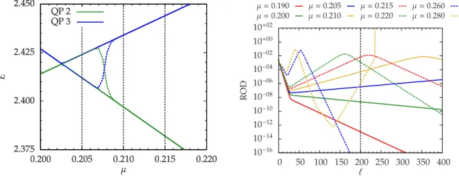
To assess the level of convergence realized by the particle-sorting generators during the integration, it is advantageous to measure the residual off-diagonality (ROD) of the Hamiltonian in the sense of terms that have to be rotated away by the generator. In this thesis, we use the Pythagorean sum of the Hamiltonian’s coefficients of all terms that contribute to the generator

ROD = s

X

i

|ηi|², (2.20)

that differs from Reischl’s original definition [Reischl et al.(2004),Reischl(2006)] by a square root. For lattice systems, it is necassary to consider the coefficients of terms related by translation invariance in the sum only once in order to guarantee a finite ROD.

The formulation in second quantization can be extended straightforwardly to observables

O(`) = X

i

oi(`)Bi (2.21)

with coefficients oi(`), while the corresponding operator basisBi does not need to be the same as for the Hamiltonian. Hence the flow equation for an observable (2.6) leads to a DES for its coefficients

∂`oi(`) = X

j,k

D_ijk^obshj(`)ok(`). (2.22a)

(22)

H

η ∂ ^ℓ H

O

η ∂ ^ℓ O

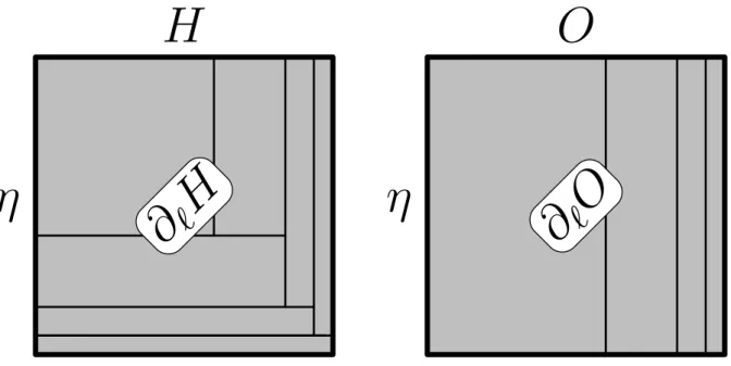
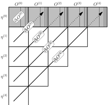
Figure 2.1: Schematic representation of the sCUT self-consistency loops. The sets of monomials are represented by the sides of the rectangle, while each area represents the set of commutators between pairs of monomials. The inner lines separate the different iterations of the sCUT algorithm. Left panel: Self-consistency loops for the Hamiltonian. Usually, both H and η refer to the same operator basis. Right panel: Self-consistency loops for an observable.

The contributions D^obs_ikj are obtained by calculating the commutators between the monomials of the generator and the monomials of the observable followed by a comparison of the coefficients

X

i

D^obs_ijkBi = [ˆη[Aj], Bk]. (2.22b) The DES for the coefficients of the observables is linear, but it is coupled to the transformation of the Hamiltonian via the prefactors hj(`).

2.4 Self-similar truncation

The characteristic approximation of the sCUT method consists in restricting the flowing Hamiltonian to a finite set of basis operators{Ai}, denoted astruncation scheme. By this, the flowing Hamiltonian is confined to a finite-dimensional sub-manifold of the operator algebra. All commutators between the relevant {Ai}are taken into account to determine the DES. Technically, this is done by calculating all the commutators for monomials present in the initial Hamiltonian first. If further monomials compatible with the truncation scheme arise in the calculation, they are added to the set of basis operators and the missing commutators are calculated. This step is iterated until no new basis operators incorporated by the truncation scheme arise [Reischl(2006),Duffe(2010)]. A schematic representation is given in Fig. 2.1. The sCUT strategy is optimal in the sense that the truncated flow is chosen as close to the untruncated flow-line as possible without violating the truncation criterion, i. e., the Frobenius/Hilbert-Schmidt norm of the neglected part of the flowing Hamiltonian is minimal for each value of ` [Moussa(2010)].

(23)

2.4 Self-similar truncation 23

α β γ

|αβγihαβγ|

α α

β β

γ γ

1

α α

β β

γ γ

a^†_αaα

α α

β β

γ γ

a^†_βaβ

α α

β β

γ γ

a^†_γaγ

α α

β β

γ γ

a^†_αa^†_βaαaβ

α α

β β

γ γ

a^†_βa^†_γaβaγ

α α

γ γ

β β

a^†_αa^†_γaαaγ

α β γ

α β γ a^†_αa^†_βa^†_γaαaβaγ

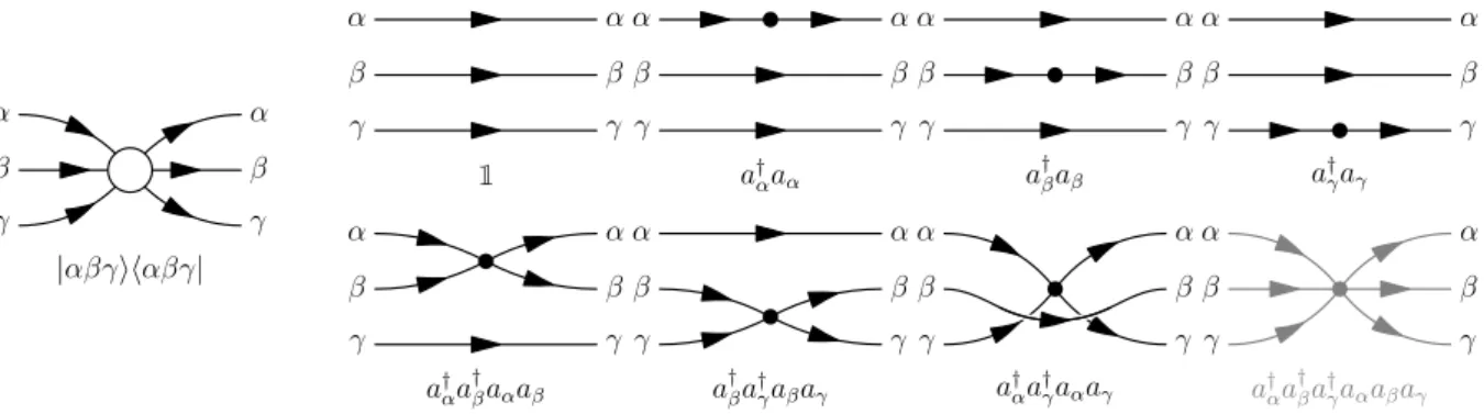
Figure 2.2: Decomposition of the diagonal matrix element|αβγi hαβγ|of a three quasi-particle state into irreducible interaction processes, cf. Ref. [Drescher et al.(2011)]. A restriction to at most two quasi-particle processes neglects only the irreducible three quasi-particle contribution a^†αa^†_βa^†γa_αa_βa_γ.

0:0

0:1

0:2 d2

0:3 d3

1:0

1:1 d2

1:2 d3

1:3 d4

2:0 d2

2:1 d3

2:2 d4

2:3 d5

3:0 d3

3:1 d4

3:2 d5

3:3 d6

N

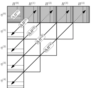
Figure 2.3: Graphical representation of the truncation schemed = (d₂, . . . , d_2N) with N = 3 for the Hamiltonian. The maximal extensionsd₀ andd₁ are superfluous since the corresponding monomials have extension zero.

(24)

We stress that the restriction to a finite set of monomials doesnot imply a restriction to a finite Hilbert space. As illustrated in Fig.2.2, the truncation of irreducible processes involving a large number of quasi-particles does not mean that matrix elements between such states would be neglected completely. Instead, the contributions of low-particle processes are used as an approximation for the matrix element and only the corrections by complicated processes (involving more particles) are neglected.

The definition of a suitable truncation scheme is a demanding task. In an early work, Kehrein and Mielke suggested the restriction to the monomials present in the initial Hamiltonian. After a solution of this minimal flow equation system, new monomials are assessed one-by-one whether taking them into account changes the solution of the flow equation significantly [Kehrein & Mielke(1994)]. However, this strategy appears to be practical only for very small systems of flow equation.

One consequence of truncation is the loss of unitarity of the transformation. As a rule of thumb, the effective Hamiltonian is believed to be the more accurate the more monomials are taken into account. A mathematical analysis of the truncation error is possible by decomposing the untruncated flow equation (2.4) forH(`) =H⁰(`)+H⁰⁰(`) into a truncated flow equation for the truncated HamiltonianH⁰(`) and an inhomogeneous flow equation for the difference to a unitarily transformed HamiltonianH⁰⁰(`) [Drescher(2009), Drescheret al.(2011)]. Eventually, this leads to a rigorous, upper bound for||H⁰⁰(`)||and for the error of the ground state energy. We stress that these quantities are accessible from within the truncated calculation. In the models analyzed so far however, these bounds turned out to be to loose for practical applications.

For practical purposes, the best possibility to estimate the quality of a truncation scheme remains to compare the results with other, more or less strict truncation schemes and with results of other numerical methods.

For incorporating large numbers of monomials in the truncation scheme, a systematic criterion is called for. In gapped quantum systems on a lattice, real-space correlation functions decay exponentially on a length scale ξ, called correlation length. This suggests the range of interactions in real-space as a criterion for the truncation scheme [Reischl et al.(2004)]. The correlation length and the gap

∆∝ξ⁻^z (2.23)

are linked by the dynamical critical exponentz [Sachdev(1999a)]. Close to a second order quantum phase transition, this real-space truncation has to be handled with care since the correlation length diverges and long-range processes become important.

As a measure of the real-spaceextension of a term of the Hamiltonian, Reischl proposed the maximal taxi cab distancedbetween pairs of local creation and annihilation operators of the monomial [Reischl(2006)]. The absolute positions are not taken into account, because, usually, the Hamiltonian is invariant under translation. In one dimension, this corresponds to the distance from the leftmost to the rightmost local operator of the monomial.

Furthermore, it is advantageous to distinguish between simple operators affecting few quasi-particles, that are expected to be most important for the low-energy physics, and complex operators affecting many quasi-particles, that are more numerous for the same extension, but influence the low-energy scale only indirectly due to their renormalizing effect to the simple operators. A more sophisticated real-space truncation scheme trun- cates monomials based on their real-space extension, the number of creation operators i and the number of annihilation operators j of the monomial [Reischl(2006),Fischer

(25)

2.5 Symmetries 25 et al.(2010)]. Ifi orj exceed the maximal particle numberN, the monomial is truncated immediately. Otherwise, a truncation based on a maximal extension dn specific for the sum n =i+j ≤2N of local creation and annihilation operators present in the monomial is applied, see Fig.2.3. The 2N-tupled = (d2, . . . , d2N) serves as a shorthand notation for the truncation scheme. The maximal extensions d0 and d1 are superfluous since the corresponding monomials have extension zero and only a single coefficient is required when translation invariance is exploited.

In principle, the truncation scheme for the monomials of the observable can be defined similarly as for the Hamiltonian with different extensions if necessary. For the calculation of response functions, however, the relevant observables are usually not invariant with respect to translations, but are confined to a specific set of lattice sites at ` = 0. In this situation, Reischl used the sum of distances between the central site and all local operators as extension of the monomials [Reischl(2006)].

Again, we have to emphasize that the restriction to a finite real-space extension of operators in second quantization does not imply a restriction to a finite Hilbert size or, in particular, to a lattice of finite size. However, a closer look [Drescher(2009),Drescher et al.(2011)] reveals that the existence of a maximal extension dmax for monomials can disguise the difference between the thermodynamic limit and a sufficiently large, but finite, system with periodic boundary conditions. While both systems are invariant with respect to translations, the periodic boundary folds back terms from the commutator (2.19b).

Due to the finite extension of representatives enforced by truncation, all consequences of these wrap-around effects are suppressed if the system size exceeds

Lfin = 3dmax+ 1. (2.24)

In this way, the truncated calculation for infinite lattices yields the same flow equations as the calculations for finite size systems with system size L > Lfin. Therefore Lfin can be understood as an effective system size induced by real-space truncation.

Yet, this effective system size addresses the quantitavive impact on the coupling con- stants of the effective Hamiltonian only. We emphasize that it is fundamentally distinct from the finite system size of, for instance, a numerical exact diagonalization (ED), which leads to a large but finite set of discrete eigenvalues. The sCUT calculation in real-space, in contrast, refers on the thermodynamic limit and must be evaluated on an infinite lattice. As a result, the sCUT calculates states of multiple quasi-particles as true continua, not as a set of discrete eigenvalues.

2.5 Symmetries

The selection of a truncation scheme is a trade-off between accuracy and computational effort, because both memory and runtime increase with the number of basis operators {A_i} of the Hamiltonian. Exploiting the symmetries of the Hamiltonian, this number can be reduced significantly, increasing the efficiency of the calculation and allowing more involved calculations. For a treatment in the thermodynamic limit, it is essential to exploit at least translation invariance.

A detailed discussion of the utilization of symmetries can be found in the PhD thesis of Alexander Reischl [Reischl et al.(2004)]. Here, we present an alternative formulation that is closer to the computational implementation realized in the program by Sebastian Duffe [Duffe(2010)].

(26)

2.5.1 Symmetries of the Hamiltonian

The presence of symmetries in the Hamiltonian appears in the algebraic representation as constant ratios between the coefficients of different monomials. The first step to exploit this redundancy is to choose polynomials as basis operators Ai, i. e., linear combinations of monomials obeying the associated symmetries. In this way, the information about multiple monomials can be encoded in a single coefficient hi. In a second step, the symmetric polynomial can be expressed by a superoperator Σ that restores the wholeb polynomial Ai dynamically from a single monomial Ci

A_i =ΣCb _i. (2.25)

Only the representative C_i has to be stored. Even more, we will see that also the derivation of flow equations can be formulated based on such representatives instead of the complete monomials. This greatly reduces the computation time. The efficiency of this step depends on the exploited symmetry group and a weight factorwcounting the number of monomials present in Ai. In particular, it is specific to the actual interaction process.

A highly symmetric representative (e. g. the identity operator 1) may be identical with its symmetric combination A_i, which yieldsw= 1. On the other hand, the polynomialA_i may be composed of up tow=nmonomials if the symmetry group of the Hamiltonian is n-fold and each individual monomial does not share any of the Hamiltonian’s symmetries.

Usually, the latter case applies to the vast majority of representatives [Duffe(2010)], which means that nearly a factor of n in the number of representatives for the Hamiltonian can be saved.

Now, we want to derive a formal description for symmetries. LetTb be a linear superoperator that acts on the vector space of monomials and satisfies the conditions

Tb(C1C2) =

T Cb 1 T Cb 2

, (2.26a)

TbbηC1 =ηbT Cb 1. (2.26b)

If Tb and ηb do not commute, this indicates that the generator scheme and the unitary transformation break the symmetry of the Hamiltonian. We speak of ann-fold symmetry transformation of the Hamiltonian if

T Hb =H, (2.27a)

Tbⁿ=1 (2.27b)

hold. Eventually, the superoperator

Gb_T :=

n

X

i=1

Tbi

(2.28) defines a sum over a subgroup of the symmetries of the Hamiltonian. If the Hamiltonian has multiple independent symmetries, the full symmetry operation can be realized by a product of sums over independent subgroups.

Applying Gb to a representative Ci generates a polynomialAi that is invariant under application of Tb as required by Equation (2.27a). As an example, let us consider a basis of local operatorsa^†_r, a_r with rbeing the one-dimensional site index. Let the Hamiltonian be symmetric with respect to the reflection superoperator Tbreflect :a⁽r^†⁾→a⁽₋^†_r⁾. Therefore,

(27)

2.5 Symmetries 27 we can use the polynomial Ai = a^†_ra_r+1+a^†_−ra₋_r₋₁ as an element of the operator basis.

It can be generated from the representative Ci =a^†_ra_r+1 by application of Gbreflect.

But if the representative shares symmetries with the Hamiltonian, each monomial may be generated multiple times. For example, take the representative Cj =a^†₀a₀ that is symmetric with respect to reflections

GbreflectCj = 2Cj. (2.29)

Consequently, the prefactor of the representative C_j in the polynomial Gb_reflectC_j is not given by unity, but by an integer m = 2, denoted as multiplicity. It is linked to the weight factor by n = m ·w. For convenience, we define the superoperators Mc and cW that express the multiplication of a monomial by the corresponding multiplicity or weight factor, respectively. The major difference to the formulation of Reischl [Reischl(2006)] is that the implementation used here relies on the normalized symmetry group operation Σ, that generates each monomial just once. In this way, it is guaranteed that a represen-b tative Ci and the corresponding monomial in Ai always share the same prefactor³. Both formulations are equivalent, but result in different intermediate correction factors in the algorithms to determine the DES. The two symmetry group operations are linked by

Gb=McΣ.b (2.30)

For this convention, the definition of the ROD from Eq. 2.20 in terms of the coefficients ηi of the representatives in the generator reads

ROD = s

X

i

wi|ηi|². (2.31)

We have to stress that all symmetries covered by this formulation occur on the level of individual monomials in second quantization. Usually, there is no exact correspondence to the unitary transformations U that leave the Hamiltonian invariant, especially for continuous symmetries. In particular, this means that only a part of the redundancy can be eliminated depending on the algebraic representation. On page 114, we discuss an example for the SU(2) spin symmetry.

The last ingredient in our formalism is the superoperatorRbthat maps each monomial to the corresponding representative. The explicit choice of the representative is arbitrary, but has to be unique. Technically, this can be implemented by generating the whole polynomial using Σ, sorting the monomials according to a suitable criterion and pickingb the first one. Eventually, we find the following relations for products of superoperators:

GbGb=nGb GbRb=Gb GbbΣ =WcGb =nbΣ (2.32a) RbGb=nRb RbRb=Rb RbΣ =b WcRb (2.32b) ΣbGb=cWGb =nΣb ΣbRb=Σb ΣbΣ =b McΣ.b (2.32c) Finally, we derive the modified version of Eq. (2.19b) for representatives. We replace the polynomials Ai by the application of the symmetry group operation on the representatives

X

i

D_ijkΣCb _i =h

bηbΣC_j,ΣCb _ki

=Gb

"

ηbGb McC_j, 1

McC_k

#

. (2.33)

3 It turns out for the symmetries used in this thesis that all monomial belonging to a symmetric combination have the same absolute prefactor, but their sign may differ.

(28)

In this equation, we expressed the division by the multiplicity of the representative Ck

by the inverse of the multiplicity superoperator. This is straight forward, because the multiplicity of a term is always a positive integer number. One of the symmetry group operations has been shifted in front of the commutator since

h

GCb 1,GCb 2

i=

n

X

i=1 n

X

j=1

TbⁱC1 Tb^jC2

−

Tb^jC2 TbⁱC1

(2.34a)

=

n

X

i=1 n

X

j=1

Tb^j

Tb^i−jC1

C2

−Tb^j C2

Tb^i−jC1

(2.34b)

=Gbh

GCb 1, C2

i. (2.34c)

Next, we take the representatives on both sides of the equation applying Rb and obtain X

i

DijkW Cc i =nRb

ηbΣCb j, 1 McCk

, (2.35)

with the final result

X

i

D_ijkC_i =X

jk

McRb

ηbΣCb _j, 1 McC_k

. (2.36)

Compared to the bare calculation, the symmetrized evaluation of the commutator involves the construction of the symmetric combination for the generator terms. This increases the number of terms on the right hand side of the flow equation by approximately n.

Nevertheless, the index set of j and k is smaller by a factor of n each, so that an overall reduction of computational effort by a factor of n can be expected.

A special case of a twofold symmetry on the operator level is the self-adjointness of the Hamiltonian. The adjoining superoperatorTb=†violates both conditions (2.26), because adjoining reverts the order of operators and does not commute, but anti-commutes with the generator scheme

{†,ηb}= 0, (2.37)

sinceηbexchanges hermitian by anti-hermitian operators. However, both sign factor cancel out in the derivation of the symmetrized flow equation (2.36), so that it holds also for this kind of symmetry.

2.5.2 Symmetries of the observable

If observable and Hamiltonian share the same symmetry group, the Equation (2.36) can be adopted for the transformation of observables, see Eq. (2.6), in a straightforward way.

However, the situation becomes more complicated if both symmetry groups differ, because the multiplicities depend on the symmetry group. In general, the symmetry group of the observable is a subgroup⁴ of the symmetry group of the Hamiltonian

GbH =GbTGbU GbO =GbT (2.38)

4 On the other hand, symmetry of an observable that is not shared by the Hamiltonian will be broken for` >0 anyways since the generator of the CUT is determined by the Hamiltonian.

(29)

2.6 Technical implementation 29

with

GbT =

nT

X

i=1

Tbⁱ GbU =

nU

X

i=1

Ubⁱ. (2.39)

It is important that the common symmetry subgroup operation GbT is applied to H after GbU in Eq. (2.38) since both do not need to commute. In the following, we use the notation D_i for a representative belonging to the operator basis of the observable. With these assumptions, the symmetry group operator GbO can be shifted as

h

GbHηCb 1,GbOD2

i =GbT

h

GbTGbUbηC1, D2

i =GbO

h

GbHηCb 1, D2

i. (2.40)

Finally, the observable transformation for representatives reads X

i

DijkDi =X

jk

McORbO

ηbΣbHCj, 1 McO

Dk

. (2.41)

2.6 Technical implementation

The computational tasks associated with the application of the CUT method can be divided into three consecutive steps:

Algebraic part: The algebraic part consists in the construction of the DES and the operator basis {Ai}, see Eqs. (2.19b) and (2.22b). Its implementation comprises most of the methodological and model-specific know-how of the sCUT method and will be the subject of this section.

Integration part: The integration part consist in solving the DES numerically to determine the coefficients of the effective Hamiltonian, see Eqs. (2.19b) and (2.22b). The integration is carried out by standard Runge-Kutta integration algorithms⁵ with both fixed (rk4) and adaptive step-size (Dopr853) using the implementation of reference [Press et al.(2007)]. Program runs for different sets of parameters are parallelized straightforwardly using the OpenMP interface [OpenMP(2005)]. The integration program is based on an earlier version written by Sebastian Duffe [Duffe(2010)] and Tim Fischer [Fi- scher(2012a)] with extensions by myself during my diploma work [Drescher(2009)]. Be- cause the numerical integration for a fixed set of parameters is straightforward and a pure numerical task, we do not explain the program in detail. However, some analyses require a more sophisticated workflow, e. g., the combination with minimization and derivation algorithms, which we will mention in due time.

Analysis of the effective Hamiltonian: After the effective Hamiltonian has been obtained, further processing is required to obtain the relevant physical quantities. The computational effort for this step varies strongly depending on the quantities of interest and may include both algebraical and numerical aspects. For instance, the ground state energy can be read off directly as the coefficient of the identity operator, while the calculation of spectral densities involves the calculation of many matrix elements and a Lanczos tridiagonalization. We will explain the different analysis tools later in the chapters where they are used.

5 A test with the Bulirsch-Stoer method [Press et al.(2007)] showed very similar results and performance as with the adaptive Runge-Kutta algorithm. It is not pursued in the following.

Variational and perturbative extensions of continuous unitary transformations for low-dimensional spin systems